Relativistic Viscous Hydrodynamics for High Energy Heavy Ion Collisions

Abstract

It has been over a decade since the first experimental data from gold nuclei collisions at the Relativistic Heavy Ion Collider suggested hydrodynamic behavior. While early ideal hydrodynamical models were surprisingly accurate in their predictions, they ignored that the large longitudinal velocity gradient meant that even small shear viscosity would produce large corrections to the transverse dynamics. In addition, much less was known about the equation of state predicted by lattice calculations of quantum chromodynamics, which predicts a soft region as the degrees of freedom change from quarks to hadrons but no first-order phase transition. Furthermore, the effects of late, dilute stage rescattering were handled within the hydrodynamic framework to temperatures where local kinetic equilibrium is difficult to justify. This dissertation presents a three-dimensional viscous hydrodynamics code with a realistic equation of state coupled consistently to a hadron resonance gas calculation. The code presented here is capable of making significant comparisons to experimental data as part of an effort to learn about the structure of experimental constraints on the microscopic interactions of dense, hot quark matter.

Physics

To my lovely wife and consistent source of inspiration, Sara.

Chapter 1 Heavy Ion Collisions

It has been understood for over half a century that the protons and neutrons that make up atomic nuclei have substructure. The symmetry structure of the many new particles that were being discovered in the 1950’s and 1960’s led to an elegant explanation in terms of constituent particles that Gell-Mann coined as quarks. The quark model successfully predicted the Omega baryon, so named for being the only undiscovered combination of the three quarks (up, down, and strange) that made up all known particles at the time. Since that time, heavier quarks have been theorized and discovered. Notably, the top quark was discovered by the Tevatron collider at Fermilab in collisions of protons with anti-protons at extremely high relative momentum. Such high momentum collisions, of single hadrons or of nuclei, form the experimental basis of our knowledge about the interactions of quarks and the corresponding force carriers, gluons. The accepted theory for explaining these interactions is called Quantum ChromoDynamics (QCD), which has been studied in great detail and strenuously tested over the last half century.

Among the unique features of QCD is that each quark is confined by the strong force and can never be completely separated from at least one or two partner quarks. Confinement is borne out experimentally: despite the extreme amount of energy available to separate quarks in heavy ion collisions, collider experiments only observe mesons and baryons, made up of two and three constituent quarks respectively, and never a bare quark. In QCD, this is explained by the introduction of color charge. Isolating objects with non-zero color charge is forbidden, and since quarks carry a single color charge, they can never be observed in isolation. In the opposite regime, when quarks are extremely close, they interact only weakly, a result known as asymptotic freedom. This is exactly the opposite of Quantum Electrodynamics where the bare charge is infinite and renormalization is required to reproduce couplings observable at large distances as terms are added to the perturbation series.

Since the strong force increases dramatically as quarks become separated, there is the possibility of creating a new and interesting state of matter when the average distance between quarks becomes small. Creating this new state of matter, often called the Quark-Gluon Plasma (QGP), in which the quarks are freed from hadrons and form a plasma was one of the goals of the heavy ion collisions at the Relativistic Heavy Ion Collider (RHIC), and the associated STAR (Solenoid Tracker At RHIC) and PHENIX (Pioneering High Energy Nuclear Interaction eXperiment) experiments [10]. While such a phase transition had been expected, clean experimental signatures that the transition has occurred have been somewhat difficult to isolate and, for instance, there is at present no evidence for behavior associated with a first-order phase transition. At this time, this is true even in the data from new RHIC initiative searching for the critical point in the QCD phase diagram at larger baryon chemical potential [11]. Still, significant experimental evidence suggests that the matter created at RHIC interacts strongly and collectively, notably away-side jet quenching [12, 1, 13, 14] and flow observables [15, 16, 17, 18].

Figure 1.1: Away side suppression of high transverse momentum hadrons in Au+Au collisions as compared to the same data for d+Au and p+p at constant energy per nucleon, $\sqrt{s_{\text{NN}}}=200$ GeV, as measured by the STAR experiment [1]. For interpretation of the references to color in this and all other figures, the reader is referred to the electronic version of this dissertation.

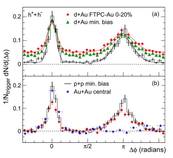
Jets are formed in hadronic collisions at high relative momentum when there is a hard scattering of a pair of quarks or gluons. If the pair scatter away from the hadronic matter, the energy due to their separation grows rapidly. The separation energy becomes much larger than the energy required to generate additional quarks and so each quark or gluon begins to form quark-antiquark pairs until they are able to form a collection of colorless combinations. This process results in a group of high momentum hadrons at small relative momentum known as a jet. In proton collisions, jets are almost always found in back-to-back pairs with similar total energy due to momentum conservation. This is not the case in heavy ion collisions, as Figure 1.1 demonstrates for Au+Au collisions at a center of mass energy per nucleon pair ($\sqrt{s_{\text{NN}}}$) of 200 GeV. The figure shows the distribution of charged particles whenever there is a very high transverse momentum particle present shown as a function of the angular difference in the transverse plane compared to that particle. To assist in interpreting this plot, we define the coordinate system of heavy ion physics. The transverse direction is radially outward from the interaction point in the plane orthogonal to the motion of the colliding nuclei, where the direction along the the motion of the colliding nuclei is referred to as longitudinal. We will frequently refer to particles by their transverse momentum, $p_{T}$, and their longitudinal rapidity, $y$. The final coordinate is the azimuthal angle in the transverse plane, $\phi$, meaning that the coordinate system in particle momentum space is cylindrical.

In Figure 1.1, the highest transverse momentum particle is defined to be at $\Delta\phi=0$ and only events with such a high transverse momentum particle are shown. Since events are selected on high transverse momentum, this particle is called the trigger particle and the associated jet is called the trigger jet. We expect a cluster of particles distributed around $\Delta\phi=0$ associated with the near-side jet, and another peak around $\Delta\phi=\pi$ corresponding to the away-side jet. This is strictly due to momentum conservation in the transverse plane. The particles in the trigger jet in the peak around zero are only slightly altered depending on the system size, but the away-side jet that appears as a peak at $\Delta\phi=\pi$ disappears for central Au+Au collisions, those that produce the largest total number of low momentum particles. This implies that the matter created in a heavy ion collisions is opaque to high momentum particles, though the theory of momentum transfer from high momentum quarks to a thermal QCD medium is not well understood [19].

Figure 1.2: The temperature extracted from blast wave fits to low mass particle spectra from the STAR experiment for various systems at various beam energies per nucleon pair [2].

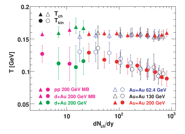
The matter created in high energy heavy ion collisions also appears to interact long enough to cool. Figure 1.2 shows the chemical and kinetic temperatures indicated by blast wave fits to the transverse momentum dependence of the particle spectra as a function of the charged particle multiplicity. In its simplest form, the blast wave model assumes that all particles were emitted from a sphere of uniform density characterized by five parameters:

• A single kinetic temperature ($T_{\text{kin}}$),

• a single chemical temperature ($T_{\text{ch}}$),

• a linear velocity profile with unknown average velocity ($\langle\beta\rangle$),

• a spherical radius (R), and

• a baryon chemical potential ($\mu_{B}$).

These five parameters are sufficient to predict the probability of observing a particular particle at a particular momentum, and therefore, they can all be determined by a fit to the spectrum low mass particles (pion, kaon, and proton). While this model is overly simplistic and does not include important physics, the parameters are a useful way of discussing trends in heavy ion collisions.

The chemical temperature extracted via the blast wave fit does not change as the number of charged particles or the beam energy increases and is consistent with the ratios observed in high energy proton-proton collisions. This trend does not carry over to the kinetic temperature indicated by the momentum distribution, which decreases as particle production increases. This softening of the spectra should not be associated with resonance production, since pions below 500 MeV/c were excluded, but instead should be related to the increasing importance of rescattering at increasingly temperatures. In peripheral collisions, which are shown in the figure as those with smaller multiplicities for the same beam energy, the spectra show no characteristic difference from proton-proton collisions in either the chemistry or the kinetics. This suggests that multiple scattering plays essentially the same role in these collisions. However, the effective kinetic temperature decreases smoothly for all beam energies as the hot region grows and the number of soft collisions, and therefore the system size, increase. This suggests that rescattering remains important for a considerable period after hadrons are created. A hydrodynamic model of heavy ion collisions must address the temperature range between kinetic and chemical freezeout. Modelers have taken two strategies – one can continue using a hydrodynamic model that takes into account the motion of the different particle species relative to one another; or one can couple the calculation to a gas model. In this work, we chose the latter.

Figure 1.3: Average particle velocity extracted from the particle spectra of heavy ion collisions of various nuclei via a blast wave fit as a function of the beam energy per nucleon pair [2]. Low momentum pions ($p_{T}<0.5$ GeV/c) are removed from the fit due to resonance background. Strong collective velocity is a strong indicator of the onset of collective behavior for collisions at center of mass energy per nucleon pair greater than a few GeV.

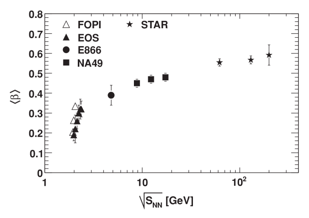
The transverse velocity indicated by the blast-wave fit is further evidence of collective behavior in heavy ion collisions. Figure 1.3 shows the average velocity indicated by the blast-wave fit as a function of beam energy per nucleon pair for heavy ion collisions. A rapid increase in the average collective velocity is observed in the region around $\sqrt{s_{NN}}=2$ GeV and a continued steady increase toward the RHIC experiments. As a baseline, the STAR experiment finds that for proton collisions at $\sqrt{s_{NN}}=200$ GeV, the apparent average collective velocity is $<\beta>_{pp}=0.24\pm 0.08$. The collective velocity in proton-proton collisions is not zero, as one might anticipate from a system expected to be too small to develop collective flow, but it is considerably smaller than $<\beta>_{AA}=0.59\pm 0.05$ as observed in heavy ion collisions [2]. This suggests that around a few GeV in beam energy the nature of heavy collisions changes, and collective response becomes critical to explaining the matter’s behavior.

Figure 1.4: Momentum dependence of the anisotropic flow observed for all charged particles by the STAR and PHENIX experiments as compared to the output of early ideal hydrodynamic simulations [3] for mid-central collisions at $\sqrt{s_{NN}}=$ 200 GeV. The simulations show excellent agreement with the experimental data up to $p_{T}=2$ GeV, where hard processes are increasingly important.

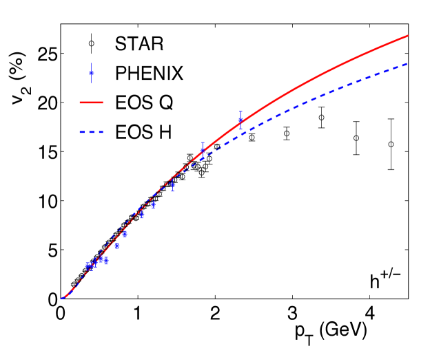
In addition to the onset of significant outward flow, the data taken at RHIC show azimuthal anisotropy of flow as shown in Figure 1.4, which shows agreement between ideal hydrodynamic models and experimental data up to $p_{T}=2$ GeV. This anisotropic (or elliptic) flow is generated by the anisotropy in the initial state from the finite impact parameter. The elliptical interaction region means larger pressure gradients along the minor axis leading to more rapid hydrodynamic expansion. This additional flow produces additional particles at moderate momenta aligned with the minor axis across a large range of rapidities and therefore the second Fourier coefficient,

$$v_{2}=<\cos{2\phi_{\text{RP}}}>,$$ (1.1)

increases where $\phi_{\text{RP}}$ is the azimuthal angle relative to the impact parameter. The agreement between ideal hydrodynamic models was considered strong evidence for the formation of the Quark-Gluon Plasma [20, 21]. At the time, there were some caveats required. Ideal hydrodynamics overestimated the duration of the collisions as seen in the longitudinal source size [22], but systematic improvements to hydrodynamic calculations have resolved these discrepancies [23]. Elliptic flow is a very important observable in heavy ion collisions and will be a focus of Chapters Five and Six.

Figure 1.5: The anisotropic flow as a function scaled by the number of quarks as a function of the kinetic energy scaled by the number of quarks [4]. This result suggests that elliptic flow is generated in the deconfined phase and is transferred to hadrons through quark recombination.

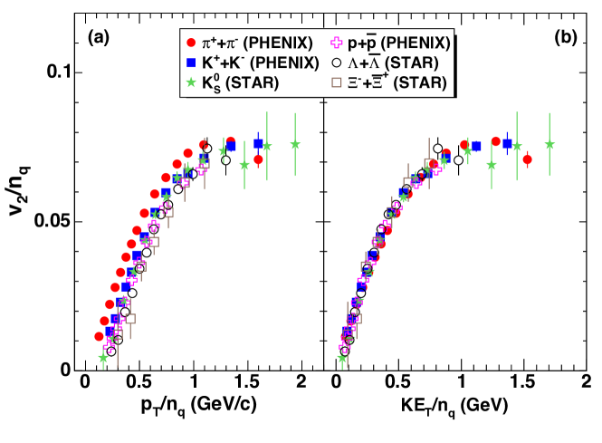
The truly novel feature of the Quark-Gluon Plasma is that quarks and gluons move freely and not in the bound particle states of a hadronic gas. While Figure 1.4 demonstrates that the matter created in a heavy ion collision exhibits hydrodynamic behavior, Figure 1.5 further shows that the anisotropic flow scales with the number of constituent quarks in the baryons and mesons observed in the final state. Scaling is not evident as a function of the transverse momentum but instead the transverse kinetic energy, $\text{KE}_{T}=\sqrt{m^{2}+p_{T}^{2}}-m$, which corresponds to the kinetic energy available after creating the particle itself. If the anisotropic flow were generated in the liquid phase, translated to the hadronic matter by recombination, and subsequent rescatterings in the gas phase did not spoil the symmetry, the quantity would be expected to be the same for all particle species. The observation that this occurs in heavy ion collisions suggests that flow is developed prior to recombination.

Figure 1.6: Baryon chemical potential indicated by particle ratios at midrapidity as measured by the STAR experiment at higher energies and other experiments at lower beam energies [2]. At beam energy of a few GeV, even the matter at midrapidity maintains the same chemical nature as the original nucleus. This is in contrast to the situation at $\sqrt{s_{NN}}=$ 200 GeV where the apparent chemical potential is reduced by almost two order of magnitude from that of stable nuclear matter.

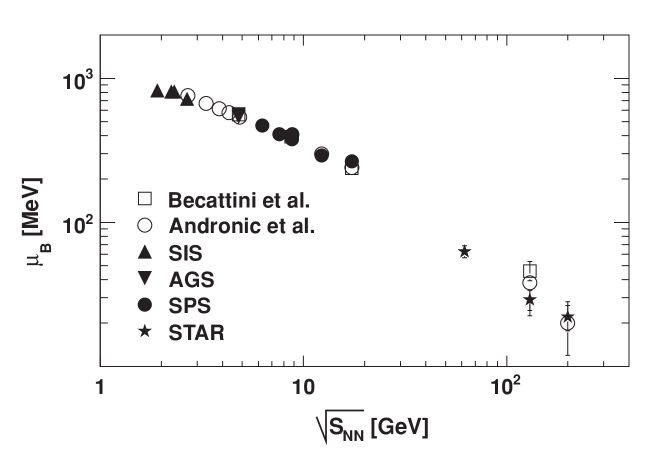
Experimental data, shown in Figure 1.6, demonstrate that the observed chemical potential in midrapidity particles is very small compared to the temperature at the highest RHIC energies. This means that there is essentially no preference in the particle ratios between baryons and mesons other than that attributable to their differing masses. Therefore, we chose a hydrodynamic description of the evolution of the quark matter that ignores the effects of non-zero baryon number. In addition to reducing computational costs slightly, there is the theoretical issue that lattice calculations are not yet able to make reliable predictions for the equation of state of quark matter at finite chemical potential. Theoretical progress on this matter is ongoing [24, 25], but in light of the significant uncertainty we choose instead to limit our experimental observables to those at midrapidity to avoid these issues.

At the onset of this project, the state of the art in hydrodynamical modeling were viscous codes with trivial longitudinal expansion based on boost invariance [26, 27, 28]. Boost invariance is based on the observation that, in the center of momentum frame, small boosts should not influence observables since the original nucleons are at much larger rapidity than the created particles [29]. If this symmetry is observed exactly, then the system will have no variation in the coordinate

$$\eta=\frac{1}{2}\log\left(\frac{t+z}{t-z}\right),$$ (1.2)

where $t$ is time and $z$ is longitudinal distance relative to the symmetry axis, which we refer to as spatial rapidity. This is due to the correspondence of spatial rapidity to momentum rapidity,

$$y=\frac{1}{2}\log\left(\frac{E+p_{z}}{E-p_{z}}\right),$$ (1.3)

where $p_{z}$ is the longitudinal momentum. This correspondence is clearest when considering the product of a particle’s momentum with the collective velocity, as will arise in the phase space density,

$$p^{\mu}u_{\mu}=\sqrt{m^{2}+p_{\perp}}\cosh{(y-\eta)},$$ (1.4)

meaning that there will be a penalty for emission at a different rapidity that scales as $\exp^{-\cosh{(y-\eta)}}$. If one defines the proper time in a frame with constant $\eta$ as a replacement for the usual lab frame time coordinate, which is defined $\tau^{2}=t^{2}-z^{2}$, one maintains an orthogonal set of coordinates with metric $g_{\mu\nu}=\text{diag}\{1,-1,-1,-\tau^{2}\}$. Furthermore, the hydrodynamic equations of motion respect boost invariance, meaning that a system born into boost invariance maintains this symmetry at all times even in the presence of shear or bulk viscosity. In the limit of infinite beam energy, the symmetry is exact.

Figure 1.7: Pion (circles) and kaon (triangles) spectrum observed by the BRAHMS experiment [5] as a function of their longitudinal rapidity including Gaussian fits (dotted lines). Shows that pion source is does not have an especially large width and boost invariance is a questionable assumption even for describing behavior at midrapidity.

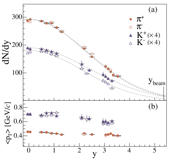
As noted earlier, for collisions at RHIC, boost invariance has proved a useful approximation for calculating midrapidity observables such as elliptic flow and particle spectra [26, 27, 28]. That said, the distribution of pions is still well described by a Gaussian in longitudinal rapidity. This was also the case at lower beam energies, though width increases to about 2.3 units of rapidity by $\sqrt{s_{\text{NN}}}=200$ GeV, as shown in Figure 1.7. While this means that boost invariance is increasingly valid, the range of validity was unknown as no three-dimensional simulation that included viscosity had been completed. In light of this, one goal of this project was to explore the validity of the boost invariant assumption in viscous hydrodynamic models regarding the prediction of midrapidity observables.

Taken in aggregate, the experimental evidence from relativistic heavy ion collisions points to the formation of a new liquid phase. This liquid remains in thermal contact long enough to develop significant radial and elliptic flow. However, the rapid longitudinal expansion means that even if the shear viscosity in the liquid phase is small, the viscous corrections to the transverse expansion will be important. For these reasons, we choose to model the high temperature regions with relativistic viscous hydrodynamics. Since larger systems cool further following the formation of hadrons, the lower temperature regions will be modeled as a hadronic gas. With this two-component model, we will investigate the sensitivity of our predictions at midrapidity to the addition of non-trivial longitudinal dynamics and uncertainties in the initial condition to hydrodynamics.

Chapter 2 Theory of Fluid Dynamics

The experimental results discussed in Chapter 1 suggest that the matter created in heavy ion collisions can be described by hydrodynamics. However, thermal contact is maintained to lower temperatures than could be described by hydrodynamics. Because of this, our model will couple an hadronic gas at low temperatures to viscous hydrodynamics at higher temperatures. The focus of this chapter will be on hydrodynamic theory underlying the higher temperature model.

In this chapter, we pursue one of the possible methods of developing fluid dynamics. We consider the macroscopic, collective behavior of systems of free moving particles interacting with one another – a highly interactive limit of a gas. This will be of particular use when coupling the hydrodynamic phase to the gaseous phase where several results from this derivation will be of direct use. While this is a useful way of deriving the equations of motion of hydrodynamics, the resulting equations are more general than a derivation from kinetic theory might imply. Most notably, the quark-gluon plasma is expected to be strongly-interacting, while kinetic theory is weakly-interacting. The equations of motion apply to systems where entropy is conserved locally, collective motion is sufficient to describe the dynamics of interest, and the acceleration of that collective velocity comes from the absence or presence of material nearby. The equations are useful only when one can express an equation of state to close the set of equations. For the case of ideal hydrodynamics with no charges, this is to provide the pressure as a function of energy density.

2.1 Kinetic Theory and Fluids

In the case of relativistic heavy ion collisions, the underlying microscopic theory at high temperature should be Quantum ChromoDynamics for a bulk system. The present state of the theory has not produced a dynamical theory evolving microscopic degrees of freedom that would be needed to describe the observations from heavy ion collisions, but it has produced an equation of state for hot quark matter from lattice models (see Chapter 3) [6, 30].

The general structure of hydrodynamic theory can be derived from breaking the system into a system of fluid elements, each of which contains many colliding particles [31, 32, 33, 34]. If the particles collide relatively infrequently, the system is dominated by particle diffusion; whereas fluid dynamics considers a system for which particles collide on a shorter time scale than the system’s shape changes. The frequent collisions will tend to move the distribution of particle momenta toward the equilibrium distribution as collisions randomize each particles’ momentum. In the case that quantum corrections to this distribution are not important, this momentum distribution is the Maxwell-Boltzmann distribution, given by

$$f(p_{\mu}u^{\mu})\propto\frac{d^{6}N}{d^{3}rd^{3}p}\propto\exp(-p_{\mu}u^{\mu}/T),$$ (2.1)

where $f$ is the phase space distribution, $p$ is the particle momentum, $u$ is the fluid velocity, and $T$ is the temperature.

The phase space distribution leads to the number density current and to the stress energy tensor. For the number density, one integrates over all momentum modes, which we will denote by

$$\int d\omega=\int\frac{d^{3}p}{(2\pi)^{3}p_{0}},$$ (2.2)

where $p_{0}$ is the relativistic energy. Using this notation, one can then define the number density current to be

$$n^{\mu}=\int d\omega~{}p^{\mu}f(p\cdot u),$$ (2.3)

and the stress energy tensor to be

$$T^{\mu\nu}=\int d\omega~{}p^{\mu}p^{\nu}f(p\cdot u).$$ (2.4)

For a collisionless system, the phase space density is conserved in the frame that moves with the particle’s momentum, $p^{\mu}$. If the particles are allowed to collide, these can be included as a source term to the equation called the collision integral. This is summarized by

$$p^{\mu}\partial_{\mu}f(u^{\mu}p_{\mu})=\it{C},$$ (2.5)

where $\it{C}$ describes the effects of collisions. This equation is often referred to as the Boltzmann equation, though it has many names depending upon the addition of other effects. It is generally considered the starting point for kinetic theory and is fundamental to the description of gases.

As described above, hydrodynamics can be seen as a limit of kinetic theory where collisions do not allow the system to significantly deviate from the equilibrium distribution. If one then integrates the Boltzmann equation over momentum, one obtains

$$\int d\omega~{}p^{\mu}\partial_{\mu}f=\partial_{\mu}n^{\mu}=0=\int d\omega~{}\it{C},$$ (2.6)

where the expression is zero assuming that collisions are local and locally conserve particle number in the aggregate. If one takes the first moment of Boltzmann equation with respect to momentum, one obtains

$$\int d\omega~{}p^{\nu}p^{\mu}\partial_{\mu}f=\partial_{\mu}T^{\mu\nu}=0=\int d\omega~{}p^{\nu}\it{C},$$ (2.7)

which is zero if the collisions also conserve momentum and energy. Higher moments of the Boltzmann equation also vanish exactly if the system never deviates from local equilibrium. This defines the stress energy tensor ($T^{\mu\nu}$) from the perspective of kinetic theory which will serve as our connection to hydrodynamic theory, most notably when coupling the hydrodynamic module to the gaseous module.

In order to calculate the connection with hydrodynamics, we consider a small volume of particles distributed according to the equilibrium distribution with no collective motion. If we calculate $T^{tt}$ from kinetic theory as in Eq. 2.4, we obtain

$$T^{tt}(\vec{r})=\int\frac{d^{3}p}{p_{0}}p_{0}^{2}f(\vec{p},\vec{r})=\epsilon,$$ (2.8)

where $\epsilon$ is the energy density. Since this frame is defined by having zero net momentum, all off-diagonal elements of the tensor are zero at equilibrium in this frame due to symmetry. Spatial elements along the diagonal, however, are proportional to the average of a momentum squared, which is non-zero and given by

$$T^{xx}(\vec{r})=\int\frac{d^{3}p}{p_{0}}p_{x}^{2}f(\vec{p},\vec{r})=P,$$ (2.9)

where $P$ is the pressure. The identification of this quantity as the pressure can be understood by noting that the linear momentum transferred to the boundary of the fluid element and the frequency of collisions with the boundary are both proportional to the momentum [31]. This will be confirmed later when we investigate the conservation of stress-energy in the following section.

One can also note directly from Eq. 2.8 and Eq. 2.9 that the equation of state for a massless gas is entirely determined. From relativistic kinematics one knows that

$$p_{0}^{2}-\vec{p}\cdot\vec{p}=m^{2},$$ (2.10)

where $m$ is the mass of the particle. But then if one examines the trace of $T^{\mu\nu}$,

$$T_{\mu}^{\mu}=T^{tt}-T^{xx}-T^{yy}-T^{zz}=\int\frac{d^{3}p}{p_{0}}(p_{0}^{2}-p_{x}^{2}-p_{y}^{2}-p_{z}^{2})f(\vec{p},\vec{r})=0,$$ (2.11)

where the final step uses the fact that the particles are massless. Changing from the kinetic theory description to the language of hydrodynamics, Equation 2.11

$$\epsilon=3P,$$ (2.12)

which suffices to provide an equation of state for ideal hydrodynamics. Note also that if the mass is non-zero, then the trace of the stress-energy tensor is positive and the pressure at constant energy density is reduced. This is relevant for temperatures larger than the pion mass where more mesonic and baryonic states become relevant and the equation of state begins to soften (Chapter 3).

2.2 Ideal Hydrodynamics

The equations of relativistic hydrodynamics can be determined by adding the requisite relativistic structure to the stress-energy tensor. The only available non-scalar quantities are the velocity of the frame in which the fluid element has no collective velocity and the metric tensor. No derivatives are permitted in the stress energy tensor since their inclusion would require the introduction an additional microscopic length scale over which we assume that the stress energy tensor will not vary. Easing of this assumption will come in the form of viscous corrections to be discussed in later sections. From our earlier symmetry consideration, the stress energy tensor has no off-diagonal structure and trace reads $T^{\mu\nu}=\text{diag}\{\epsilon,P,P,P\}$ in the frame with no collective velocity. This is sufficient to determine the relativistic structure [32], which for ideal hydrodynamics is given by

$$T^{\mu\nu}=u^{\mu}u^{\nu}(\epsilon+P)-g^{\mu\nu}P,$$ (2.13)

where $u^{\mu}$ is the collective velocity and $g^{\mu\nu}$ is the metric tensor. We take the metric to be $T^{\mu\nu}=\text{diag}\{1,-1,-1,-1\}$ in Minkowski space, and $u^{\mu}$ transforms as a vector and has unit measure, $u_{\mu}u^{\mu}=1$. Implicitly, we have chosen the Landau frame where the collective velocity moves with the energy density, and not the Eckhart frame where the collective velocity moves with particle number. This is due in part to interest in systems with zero net charge where particle number, and therefore the Eckhart frame, would not be well defined.

The equations of motion of ideal hydrodynamics are then just the conservation of the stress energy tensor as from Eq. 2.7. The portion of temporal component along the collective velocity is given by:

$$0 = u_{\nu}\partial_{\mu}T^{\mu\nu}=u_{\nu}\partial_{\mu}\left[u^{\mu}u^{\nu}(\epsilon+P)-g^{\mu\nu}P\right],$$

$$0 = D\epsilon+\left(\epsilon+P\right)\partial_{\mu}u^{\mu},$$ (2.14)

where $D=u^{\mu}\partial_{\mu}$ is the comoving time derivative. To obtain the familiar non-relativistic limit, assume that $v^{2}$ is small and that $\gamma\approx 1$. This yields the familiar expression:

$$\partial_{t}\epsilon+\vec{v}\cdot\vec{\nabla}\epsilon=-(\epsilon+P)\vec{\nabla}\cdot\vec{v}.$$ (2.15)

The divergence of the collective velocity is often called the expansion rate and can be related to the change in volume of the fluid element by $dV/dt=V\vec{\nabla}\cdot\vec{v}$. Equation 2.15 can then recast as $dE=-PdV$ which is the fundamental thermodynamic relation for a system with constant entropy. For this reason, the first equation of ideal hydrodynamics is often framed in terms of the local conservation of entropy. Furthermore, it underscores the more general applicability of hydrodynamics to statistical systems at or near the maximal entropy state.

The Euler equation is related to the conservation of the spatial elements of the stress-energy tensor. To extract this independently of the first equation we use the projector $\Delta^{\mu\nu}=g^{\mu\nu}-u^{\mu}u^{\nu}$ which selects out the spatial indices in the frame of the matter. Applying this to the equation of stress-energy conservation yields

$$0 = \Delta^{\alpha}_{\nu}\partial_{\mu}T^{\mu\nu}=\partial_{\mu}T^{\mu\alpha}-u^{\alpha}\left(D\epsilon+(\epsilon+P)\partial_{\mu}u^{\mu}\right),$$

$$0 = (\epsilon+P)Du^{\alpha}+u^{\alpha}DP-g^{\alpha\mu}\partial_{\mu}P.$$ (2.16)

When taking the same limit as before, one obtains

$$(\epsilon+P)\partial_{t}\vec{v}+(\epsilon+P)\left[\vec{v}\cdot\vec{\nabla}\right]\vec{v}=-\vec{\nabla}P-\vec{v}\partial_{t}P,$$ (2.17)

which reduces to $(\epsilon+P)\partial_{t}\vec{v}=-\vec{\nabla}P$ in the frame of the matter. This should be interpreted to mean that acceleration of the frame of the collective velocity is due to the pressure gradient observed in that frame.

2.3 Viscous Hydrodynamics

2.3.1 Navier-Stokes Hydrodynamics

The equations of ideal hydrodynamics are derived from the assumption that local equilibrium is exact, or equivalently, assuming that the mean free path of the microscopic particles is identically zero. If this is the case, a uniform density fluid with a plane of static fluid adjacent to a plane of fluid in motion would be a stable condition; the two planes would never affect one another because only the divergence of the collective velocity, rather than a mixed partial derivative like $\partial_{y}v^{x}$, enters into the equations of motion. That is, pressure is a force orthogonal to the surface of the fluid element in the rest frame; shear viscosity allows force along the surface.

Experience with liquids indicates that this is not a physical conclusion; if one pulls a sheet of material through a fluid, nearby fluid begins to move with the sheet. Friction in the fluid allows linear momentum to be transferred between adjacent fluid elements and their collective velocities would tend to equalize. Navier-Stokes hydrodynamics introduces a viscous correction to the spatial elements of the stress-energy tensor from such a frictional force [31]. Physically, this should be separated into a traceless contribution and an effect on the trace, which correspond to shear ($\eta$) and bulk ($\zeta$) viscosity respectively. The viscous components are proportional to the velocity gradient with a corresponding transport coefficient that characterizes the amount of internal friction in the fluid. In the traceless case, this the shear viscosity. These results can be summarized as

$$\delta T^{ij}\propto\eta\frac{\partial v^{i}}{\partial x^{j}},~{}~{}\delta T^{ij}\propto\zeta\delta^{ij}\vec{\nabla}\cdot\vec{v}.$$ (2.18)

These terms are collected into a correction to the stress energy tensor – $\pi^{\mu\nu}$ – and referred to as the shear tensor. The shear tensor is mostly clear written in the fluid frame where it takes the form

$$\pi^{ij}=-\eta\left(\partial_{i}v^{j}+\partial_{j}v^{i}-\frac{2}{3}\delta^{ij}\vec{\nabla}\cdot\vec{v}\right),$$ (2.19)

where $\delta^{ij}=1$ if $i=j$ and is otherwise zero, and the latin indices are meant to indicate that this applies only to spatial coordinates. In the frame of the matter, the ideal part of the stress energy tensor is only the outward pressure, $\delta^{ij}P$, and Eq. 2.19 is added as a correction to the equations of motion (Eqs. 2.15 and 2.17). These additions result in the Navier-Stokes equations of viscous hydrodynamics. Note that adding these corrections relativistically is non-trivial as one needs to correct for both the frame motion in both the derivatives and the velocities. This will be addressed fully when discussing the Israel-Stewart equations of motion.

2.3.2 The Maxwell-Cattaneo Equation

Solving the Navier-Stokes equations is notoriously difficult as the differential equations are parabolic, for which solutions tend to be unstable, and famously unsolved in the general case. In addition to being difficult to solve, the relativistic Navier-Stokes equations are not necessarily causal as the system responds instantaneously to changes in the velocity gradients.

While it is not clear that either of these difficulties are important for heavy ion physics, both can be addressed within the Maxwell-Cattaneo framework [32]. Essentially this framework assumes that instead of defining the change to the effective pressure to be exactly proportional to the velocity gradients, it instead relaxes toward the Navier-Stokes value. This means that the shear tensor can no longer be computed directly from the other dynamical variables or their derivatives. Therefore, the shear tensor itself is promoted to a dynamical variable and must be tabulated separately. In addition, the shear tensor now must have its own equations of motion. The form of these equations of motion in the frame of the matter are taken to be of the form

$$\partial_{t}\left(\frac{\pi^{ij}}{\sigma_{\eta}}\right)=\frac{-\left(\pi^{ij}-\pi^{ij}_{(NS)}\right)}{\sigma_{\eta}\tau_{\pi}},$$ (2.20)

where $\pi^{ij}_{(NS)}$ is the Navier-Stokes shear tensor given by Eq. 2.19, $\tau_{\pi}$ is a new transport coefficient that characterizes the time scale on which the system approaches Navier-Stokes viscosity, and $\sigma_{\eta}$ is a scaling factor required to guarantee the Second Law of Thermodynamics [35] (see the following subsection).

Historically, this equation informed the search for an extension of hydrodynamic theory that would would be hyperbolic and causal in the general case. The equations of motion for the shear tensor can be derived in this form from a gradient expansion in kinetic theory or from general entropy production considerations as will be shown in the next two subsections. That said, the new transport coefficients, $\tau_{\pi}$ and $\sigma_{\eta}$ will not be independent of one another complicating the correspondence of the Israel-Stewart theory to the Maxwell-Cattaneo equation and its interpretation as a relaxation equation.

2.3.3 Israel-Stewart Hydrodynamics and Entropy

Since the system is away from equilibrium, the entropy should be reduced from its equilibrium value. One expects the entropy should increase quadratically as the shear tensor increases simply from symmetry at equilibrium so the lowest order correction to the entropy current would be

$$s^{\alpha}=u^{\alpha}\left(s_{\text{eq}}-\beta\pi_{\mu\nu}\pi^{\mu\nu}\right),$$ (2.21)

where $\beta$ is a thermodynamic quantity to be determined [35]. The second term acts as an entropy source and so it must have positive four-divergence relative to the dynamical entropy from the Navier-Stokes continuity equation [32, 36]:

$$0 \leq \frac{1}{T}\pi_{\mu\nu}\nabla^{<\mu}u^{\nu>}-\partial_{\alpha}\left[u^{\alpha}\beta\pi_{\mu\nu}\pi^{\mu\nu}\right],$$

$$0 \leq \pi_{\mu\nu}\left[\frac{1}{T}\nabla^{<\mu}u^{\nu>}-2\beta D\pi^{\mu\nu}-\pi^{\mu\nu}D\beta-\pi^{\mu\nu}\beta\partial_{\alpha}u^{\alpha}\right],$$ (2.22)

where $\nabla_{<\mu}u_{\nu>}$ is the traceless part on the velocity gradient and is defined as

$$\nabla_{<\mu}u_{\nu>}=\nabla_{\mu}u_{\nu}+\nabla_{\nu}u_{\mu}-\frac{2}{3}\Delta_{\mu\nu}\partial_{\alpha}u^{\alpha},$$ (2.23)

with

$$\Delta^{\mu\nu}=g^{\mu\nu}-u^{\mu}u^{\nu},~{}~{}~{}~{}\nabla^{\mu}=\Delta^{\mu\nu}\partial_{\nu}.$$ (2.24)

This traceless part of the velocity gradient is just the Navier-Stokes modification to the pressure except the factor of the shear viscosity: $\pi^{\mu\nu}=\eta\nabla^{<\mu}u^{\nu>}$. The constraint in Eq. 2.22 must be guaranteed for any expansion with any physical transport coefficients, which can be achieved if one requires that

$$\pi^{\mu\nu}=\eta T\left[\frac{1}{T}\nabla^{<\mu}u^{\nu>}-2\beta D\pi^{\mu\nu}-\pi^{\mu\nu}D\beta-\pi^{\mu\nu}\beta\partial_{\alpha}u^{\alpha}\right].$$ (2.25)

This is an equation of motion for the shear tensor, where one should recall that $D$ is the time derivative in the frame of the matter. If $\beta$ is taken to be zero, the Navier-Stokes form for the shear tensor is recovered exactly. In addition, it can be transformed into a relaxation equation with the same structure as Eq. 2.20 via the appropriate choice for the new transport coefficient $\beta$. To show this, one can rewrite Eq. 2.25 as follows

$$D\pi^{\mu\nu}+\pi^{\mu\nu}\frac{D\beta}{2\beta}+\frac{\pi^{\mu\nu}}{2}\partial_{\alpha}u^{\alpha}=\frac{-\left(\pi^{\mu\nu}-\pi^{\mu\nu}_{(NS)}\right)}{2\eta T\beta},$$ (2.26)

which leads to two equations for the two unknowns:

$$\beta=\frac{2\eta T}{\tau_{\pi}},~{}~{}~{}~{}~{}\sigma_{\eta}D\left(\frac{\pi^{\mu\nu}}{\sigma_{\eta}}\right)=D\pi^{\mu\nu}+\pi^{\mu\nu}\frac{D\beta}{2\beta}+\frac{\pi^{\mu\nu}}{2}\partial_{\alpha}u^{\alpha}.$$ (2.27)

Since the relaxation time is a transport coefficient to be calculated from the underlying microscopic theory, the left part of Equation 2.27 gives a value for $\beta$. The right part of Equation 2.27 can be recast as a single, local conservation equation

$$\frac{D(\sigma_{\eta}\sqrt{s\beta})}{\sigma_{\eta}\sqrt{s\beta}}=0,$$ (2.28)

which is guaranteed if $\sigma_{\eta}^{-2}=s\beta$. Returning to Equation 2.21 for the viscous entropy current and noting that the probability for a given fluctuation of stress-energy is proportional to $e^{S}$, then the variance of $\pi_{xy}$ in a given volume V is

$$V<\pi_{xy}^{2}>=\frac{1}{2\beta}=\frac{s\sigma_{\eta}^{2}}{2},$$ (2.29)

meaning that $\sigma_{\eta}$ behaves like the variance of $\pi_{xy}$.

2.3.4 Israel-Stewart Hydrodynamics and Kinetic Theory

The derivation connecting Israel-Stewart hydrodynamics with kinetic theory is rather involved and the details are beyond the scope of this document, but a quick sketch is helpful for conceptual reasons. In addition, the form of the phase space distortion shown in this section will be useful later when connecting the hydrodynamic fireball to the surrounding hadronic gas.

In establishing the connection between kinetic theory and ideal hydrodynamics, we discussed the equilibrium phase space density and the Boltzmann equation. In doing so, we discussed the effect of collisions, which are a source (or sink) to the conservation of phase space density. We argued that if the collisions happened often enough, then the system would remain in equilibrium. This assumption along with energy-momentum conservation was enough to produce ideal hydrodynamics.

Further, when discussing the Navier-Stokes viscous corrections hydrodynamics, we mentioned that this can be thought of either as friction in the fluid from a macroscopic perspective, or as the effects of expansion between collisions. In particular, if one imagined a box of particles with an arbitrary distribution of initial momenta but zero total momentum, and then investigated the system at later times, the collisions would tend to relax toward the momentum distribution and the system would exponentially approach the equilibrium distribution [37, 33, 38, 39, 34]. This can be summarized as

$$\it{C}=-p_{\mu}u^{\mu}\frac{f-f_{0}}{\tau_{\pi}},$$ (2.30)

where $\tau_{\pi}$ is the relaxation time scale.

Now, hydrodynamics will not generally apply to situations where the system is far from thermal equilibrium so we concern ourselves only to the case of small deviations of the phase space density. Using the fact that this deviation should disappear in equilibrium and should only be a function of the available degrees of freedom, the simplest ansatz was proposed by Grad [40] who found that the distortion to the phase space density should be

$$f=f_{0}\left[1+\frac{\pi_{\alpha\beta}p^{\alpha}p^{\beta}}{2(\epsilon+P)T^{2}}\right].$$ (2.31)

This form of the deviation and the equation of motion for the shear tensor come from a detailed analysis of higher moments of the Boltzmann equation [41, 33, 38].

The important revelation from this approach is the possibility of additional terms that do not produce any entropy [32]. Such terms would not appear in a derivation based solely on the form of the entropy current. These additional terms tend to require even more transport coefficients many of which do not have obvious physical descriptions. The exception is the coupling of the shear tensor to the vorticity tensor, which in the frame of the matter is

$$\Omega^{ij}=\partial_{i}v^{j}-\partial_{j}v^{i},$$ (2.32)

would arise naturally from hydrodynamic considerations and does not require additional transport coefficients. This term has been included in our calculations but our studies confirm others’ results that it is not an important driver of dynamics for smooth initial condition investigations of hydrodynamical flow.

At this point, we have discussed all the important physics related to viscous hydrodynamics for the purposes of producing a simulation of zero charge heavy ion collisions. The details of the equations of motion to be integrated have been reserved for Chapter 4.

Chapter 3 Equation of State and Transport Coefficients

While hydrodynamics is a theory that applies to a wide variety of systems, both strongly and weakly coupled, the microscopic details of a fluid need to be included through the equation of state and the transport coefficients. For heavy ion collisions, two physical regimes are relevant as discussed at length in Chapter 1. At low temperature, the equation of state should be calculated as a non-interacting gas of mesons and baryons; while at high temperature, lattice QCD should be used. These predictions may not be compatible in the region near the transition between hydrodynamics and the hadron resonance gas, and care must be taken to ensure that the model is self-consistent at the boundary. This is especially important for the equation of state where, for instance, discontinuity in the pressure as a function of energy density would lead to hydrodynamic instability. While this temperature region is still under active investigation, recent lattice results suggest that the discrepancy between the two theories is not large and a composite description is possible. This is discussed in the first section of this chapter.

In the second section, we discuss the determination of transport coefficients in linear response theory. At this time, lattice calculations are not developed to the point where they can make predictions about transport coefficients using classic results like the Kubo relations. Because of this, our results will be from the weakly coupled theory at low temperature, the general expectation that shear viscosity should be small near the phase transition, and scaling arguments from scalar field theories of the high temperature phase.

3.1 Equation of State

3.1.1 Hadron Resonance Gas

The equation of state of the hadron resonance gas model is developed as a gas. If one assumes that the gas is non-interacting, one can simply generate a partition function using all the available particle states, which are measured experimentally. This ignores the finite volume or mean field effects that are well known to be important for lower energy heavy ion physics but are expected to be less important corrections at energies where zero baryon number hydrodynamics apply. Data on particle states up to several GeV/$c^{2}$ in mass are available from the Particle Data Group. We use resonances up to masses of $m=2.5$ GeV/$c^{2}$ as the addition of higher mass resonances no longer affects the equation of state up to temperatures of $T=175$ MeV. This choice leads to a nice agreement with lattice results in the transition region [42].

The partition function is calculated from the usual product of available mass states weighted by a common temperature. The contribution to the log of the partition function for a mass state $m_{i}$ is given by

$$\frac{1}{V}\ln\textit{Z}_{i}=\frac{\mp d_{i}}{2\pi^{2}}\int_{0}^{\infty}dkk^{2}\ln{(1\mp z_{i}e^{-\sqrt{k^{2}+m_{i}^{2}}/T})}$$ (3.1)

where $d_{i}$ is the spin degeneracy of the state and $z_{i}$ are the fugacities summed over all charges [6]. One can then use standard thermodynamic relations to obtain the equation of state. For instance the pressure and energy density are

$$P=\frac{T}{V}\displaystyle\sum\limits_{i}\ln{\textit{Z}_{i}},~{}~{}\epsilon=\frac{T^{2}}{V}\frac{\partial}{\partial T}\displaystyle\sum\limits_{i}\ln{\textit{Z}_{i}}.$$ (3.2)

From these, the entropy density can be calculated using the thermodynamic identity, $sT=\epsilon+P$.

To briefly summarize the results of this procedure, the hadron resonance gas acts like a pion gas for temperatures less than 100 MeV. However, the increasing number of baryon and meson states play an increasingly important role as the temperature increases. This produces an order of magnitude increase in the trace anomaly (or interaction, $I(T)=\epsilon-3P$) by 150 MeV. In fact, inclusion of the resonances in the mass range $1.0~{}\text{GeV}<m_{i}<2.5~{}\text{GeV}$ provides a factor of 3 in the trace anamoly by $T=200$ MeV [6, 30]. From a hydrodynamic perspective, this yields a soft region – with lower speed of sound – as a heating system would expend part of its energy in changing the degrees of freedom instead of increasing the pressure. This behavior is a milder version of a latent heat which would be associated with a first order phase transition, where there would be no increase in pressure over a region of increasing energy density.

3.1.2 Lattice QCD

In Lattice QCD, one also sets out to calculate a partition function as a function of temperature but within a field theory rather than a non-interacting gas. The details of this procedure are complex and involve computing path integrals over the gauge field on a discretized hypercube and extrapolating to the physical pion mass. The computational effort required for each time step is immense and computations are performed on large clusters designed specifically for the task. Developments in this area now allow for the computation of twelve time steps for $64^{3}$ spatial grid points [6, 30]. Different temperatures are investigated by altering the lattice spacing, and several spacings must be investigated to quantify convergence and protect against discretization effects.

While the lattice has produced some incredibly useful results for finite temperature QCD matter, it has important limitations. The “sign problem” complicates direct investigation of the equation of state away from zero chemical potential where there is the possibility of a critical point. There the phase transition might shift from a smooth cross-over seen at zero chemical potential to a first-order phase transition. Extrapolation toward this critical point from lattice data has been attempted via Taylor expansion [25, 24]. While one does not expect this expansion to be valid far from zero chemical potential, especially when approach a critical point, recent results suggest tentative agreement with other theories.

Figure 3.1: Trace anomaly from the lattice and from the hadron resonance gas model [6] showing the location of the critical region and agreement with the Hadron-Resonance gas equation of state at temperatures well below the critical region.

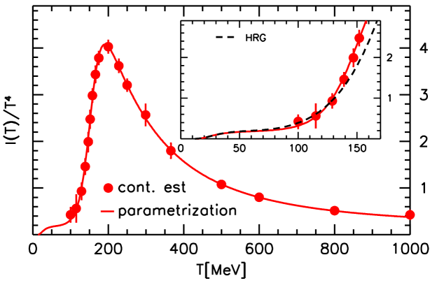
Furthermore, it is not possible to use a physical quark mass for the up and down (the lightest) quarks. The up and down quarks have physical masses of around 3-4 MeV and the strange quark around 200 MeV, but the typical lattice calculation take the mass of the up and down quarks to be a tenth that of the strange quark. This leads to a pion mass that is significantly too large. This significantly alters conclusions about the pressure in this region and generally makes interpretation of the lattice results significantly more difficult as one must extrapolate to the physical meson and baryon masses in order to extract corrected thermodynamic quantities. Despite of all this, as one finds in Fig. 3.1, there is good agreement with the Hadron Resonance Gas model for the temperature region in which one hopes both might be valid.

Also included in Fig. 3.1 is a parameterized fit to the unit-less interaction over the full temperature space. In this case [6], the fit function reproduces the HRG interaction within 7% at temperatures below 100 MeV, and calculation of the pressure via the integral method

$$\frac{P(T)}{T^{4}}=\int_{~{}0}^{T}\frac{dT^{\prime}}{T^{\prime}}\frac{I(T^{\prime})}{T^{\prime 4}}$$ (3.3)

finds deviations of only 2% and other collaborations find comparable results [30].

3.1.3 Cross-over Region

The general structure of our model is a hydrodynamic region defined by temperatures above some threshold surround by a gas of interacting hadrons. Practically, dynamic coupling of these two calculations is difficult as pressure fluctuations in the gas might easily result in extreme hydrodynamic instability. Instead, one runs the hydrodynamic simulation for a larger region of configuration space under the assumption that regions at much lower temperatures do not have undue influence on the hydrodynamical portion and that near the switching temperature the models are equivalent.

As a direct consequence, modelers should be fastidious in ensuring that the equation of state for the gas is used as precisely as possible for those regions. While lattice calculations provide a fit that includes data points from the HRG equation of state and the lattice, this may not be sufficient to ensure self-consistency. In fact, one finds that for $T=165$ MeV, lattice fits can produce energy densities that differ from the gas’ energy density by 10-20% without fundamentally different behavior in the interaction measure, $I(T)$. If left uncorrected, the hydrodynamic code would improperly emulate the gas at the boundary, and the model of particle production would fail to be self-consistent.

Since one might want to use an arbitrary lattice equation of state that might not reproduce the gas well enough, we perform a continuous merge between the two equations of state over a temperature range starting at the hadronization temperature ($T_{H}$) up to the temperature where only lattice results are used ($T_{L}$). In particular, we wish to maintain a continuous speed of sound for hydrodynamic stability, which can be written in terms of the unit-less entropy density ($\sigma=s/T^{3}$) as

$$c_{s}^{2}=\frac{dP}{d\epsilon}=\frac{1}{3+\frac{T}{\sigma}\frac{d\sigma}{dT}}$$ (3.4)

which can be derived using standard Maxwell relations. This is a clarifying expression as it points out that entropy increasing faster than $T^{3}$ is associated with softness in the equation of state, but also means that $\sigma$ is a useful variable for merging equations of state, as continuity and smoothness ensure the continuity of the speed of sound.

Figure 3.2: Unit-less entropy density in merging region. The entropy production follows that of the hadron resonance gas up to the hadronization temperature ($T_{H}=155$ MeV) and smoothly produces additional entropy to agree with the lattice entropy [6] at $T_{L}=185$ MeV.

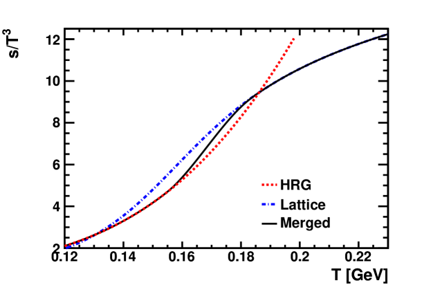
We perform the merge in the unit-less entropy density using a linear weight function that goes smoothly and continuously between the hadron resonance gas entropy ($\sigma_{H}$) and the lattice entropy ($\sigma_{L}$):

$$\sigma(T) = \left[1-w(T)\right]\sigma_{H}(T)+w(T)\sigma_{L}(T)$$ (3.5)

$$w(T) = \frac{1}{2}\left[\tanh{\left(\tan{\left[\frac{\pi}{2}\left(2\frac{T_{L}-T}{T_{L}-T_{H}}-1\right)\right]}\right)}+1\right],~{}T_{H}<T<T_{L}$$ (3.6)

and $w(T)$ is zero for $T<T_{H}$ and unity for $T_{L}<T$ and importantly also has zero slope at both $T_{H}$ and $T_{L}$ to maintain continuous speed of sound. Figure 3.2 shows the result of the procedure compared to the original equations of state and demonstrates that the procedure is continuous and smooth.

Figure 3.3: Speed of sound in merging region that results from merging in the unit-less entropy density via the produce described in the text. Note that the Lattice data [6] does not exactly follow the HRG data below the freezeout temperature due to inexact fitting. Forcing the equation of state to be exactly the HRG below the freezeout temperature lowers the entropy density at constant temperature and causes a somewhat more abrupt soft region in the transition region.

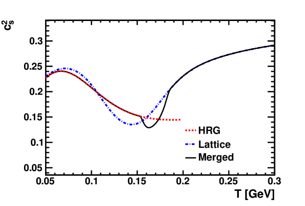
Like the hadronization temperature, the lattice-only temperature is a parameter of the model and should not be so large that gas data is being used at temperatures well above its applicability or so small that the entropy increase becomes too rapid. Figure 3.3 shows the speed of sound squared in the region of the merging procedure. Since the entropy of the hadron gas lags behind the lattice, the merging procedure gives a steeper increase for temperatures just greater than the hadronization temperature. This manifests as an even smaller speed of sound in this region. Lowering the lattice temperature while leaving the hadronization temperature the same would results in a more extreme dip in the speed of sound squared. Choosing a lattice temperature too close to the hadronization temperature could lead to an extremely soft region in the equation of state and cause hydrodynamic instabilities.

For completeness, we note that the entropy density is the temperature derivative of the pressure, $s=\frac{dP}{dT}$, so knowing the pressure of the hadron gas at $T_{H}$ and the entropy density at all temperatures allows one to get the pressure at all temperatures. Then the energy density is found from $\epsilon=sT-P$. We calculate each quantity at an interval of 1 MeV in temperature and a bookmarked search is performed each time a thermodynamic quantity is needed. Since our model does not solve the Riemann fan and cannot handle shocks, we take great care to avoid interpolation errors in the equation of state. A cubic spline [43] is performed on each of the thermodynamic variables and the interpolated values from this are used including the speed of sound squared which must be calculated as part of the splining procedure. This procedure involves a minor amount of preprocessing but the bookmarked search algorithm is unchanged and a minor part of computational time.

3.2 Transport Coefficients

As discussed in the previous chapter, viscous hydrodynamics introduces the effects of non-equilibrium to the collective response of material. In the case of shear viscosity, this can be thought of as friction within the fluid or a finite mean free path, if the underlying theory is a classical gas. The form of the correction is a small change to spatial elements of the stress-energy tensor due to velocity gradients, for example,

$$\delta T^{xy}=\eta\left(\partial_{x}v^{y}+\partial_{y}v^{x}\right).$$ (3.7)

This can be viewed in terms of Linear Response Theory where $T^{xy}$ is the operator being varied, $\eta$ is the coefficient of response, and the velocity gradients are the small field.

For the variation of some operator $A$, the variation of its expectation value due to the field can be expressed in terms of the variation of the wavefunction as

$$\delta\left\langle A\right\rangle=\left\langle\delta\psi|A(0)|\psi\right\rangle+\left\langle\psi|A(0)|\delta\psi\right\rangle=\chi F$$ (3.8)

where $\chi$ is a susceptibility and F a small external field. The change the wave function can be viewed as the result of some potential, which we assume to be related to the field by $V(t)=B(t)F$, leading to

$$|\delta\psi>=\frac{-i}{\hbar}\displaystyle\int\limits_{-\infty}^{0}dtV(t)|\psi_{0}>=\frac{-i}{\hbar}\displaystyle\int\limits_{-\infty}^{0}dtB(t)F|\psi_{0}>$$ (3.9)

so that the variation of the original operator can be written

$$\delta\left\langle A\right\rangle = \frac{-i}{\hbar}\displaystyle\int\limits_{-\infty}^{0}dt\left\langle\left[A(0),B(t)\right]\right\rangle F=\chi F,$$ (3.10)

$$\chi = \frac{-i}{\hbar}\displaystyle\int\limits_{-\infty}^{0}dt\left\langle[A(0),B(t)]\right\rangle.$$ (3.11)

In the case of shear viscosity, we are interested in the response of stress-energy to the velocity gradient. The potential associated with this is

$$V=\int d^{3}rT^{0j}r^{i}\frac{\partial v^{j}}{\partial r^{i}},$$ (3.12)

where latin indices indicate spatial coordinates. This form for the potential can be viewed as the change to the energy due to boosting to the frame of the velocity gradient [44]. This means that Equation 3.11 gives the shear viscosity to be

$$\eta=\frac{-i}{\hbar}\displaystyle\int\limits_{-\infty}^{0}dt\int d^{3}r\left\langle\left[T^{xy}(0),T^{0j}(r,t)\right]\right\rangle r^{i}.$$ (3.13)

Inserting unity in the form $\partial_{t}t$ and the integrating by parts with the correlation at minus infinity assumed to be zero,

$$\eta = \frac{-i}{\hbar}\displaystyle\int\limits_{-\infty}^{0}tdt\int d^{3}r\left\langle\left[T^{xy}(0),\partial_{t}T^{0j}(r,t)\right]\right\rangle r^{i},$$ (3.14)

$$\eta = \frac{i}{\hbar}\displaystyle\int\limits_{-\infty}^{0}tdt\int d^{3}r\left\langle\left[T^{xy}(0),T^{xy}(r,t)\right]\right\rangle,$$ (3.15)

where we have used the conservation of stress-energy, integrated by parts in the spatial coordinate disregarding the correlation at infinite range, and then noted that symmetry requires that some of the stress-energy tensor elements be the same. The commutator in Equation 3.15 can be eliminated:

$$\displaystyle\int\limits_{-\infty}^{0}t~{}dt\left\langle\left[T^{xy}(0),T^{xy}(t)\right]\right\rangle = \displaystyle\int\limits_{-\infty}^{0}t~{}dt\left(\left\langle T^{xy}(0)T^{xy}(t)\right\rangle-\left\langle T^{xy}(0)T^{xy}(-t)\right\rangle\right),$$ (3.16)

$$= \displaystyle\int\limits_{-\infty}^{\infty}t~{}dt\left\langle T^{xy}(0)T^{xy}(t)\right\rangle,$$

where we’ve ignored the spatial integration for clarity.

Producing the classical Kubo relation from this expression requires evaluating the thermal average, which is

$$G(t) = \left\langle T^{xy}(0)T^{xy}(t)\right\rangle=\text{Tr}\left[e^{-\beta H}T^{xy}(0)T^{xy}(t)\right],$$ (3.17)

$$= \text{Tr}\left[e^{-\beta H}~{}T^{xy}(0)~{}e^{iHt/\hbar}~{}T^{xy}(0)~{}e^{-iHt/\hbar}\right].$$

After analytically continuation, $G(z)$ for complex $z$ is symmetric about $z=i\beta\hbar/2$:

$$G(z+i\beta\hbar/2) = \text{Tr}\left[e^{-\beta H}~{}T^{xy}(0)~{}e^{iHz/\hbar-\beta H/2}~{}T^{xy}(0)~{}e^{-iHz/\hbar+\beta H/2}\right],$$

$$= \text{Tr}\left[e^{-\beta H}~{}T^{xy}(0)~{}e^{-iHz/\hbar-\beta H/2}~{}T^{xy}(0)~{}e^{iHz/\hbar+\beta H/2}\right]=G(-z+i\beta\hbar/2),$$

where the cyclic symmetry of the trace is used to rotate around $\exp{(-\beta H/2)}$ in Equation 3.2. Note that this result also means that $G(t+i\beta\hbar)=G(-t)$. Together these results mean that integration along the positive real axis can be performed by a complex contour integral. The integration region is taken to be rectangular with corners at $z=\{0,i\beta\hbar\}$ and extending to infinity in the positive real direction. The region is closed by a curve at infinity which disappears as long as correlations decay faster than $t^{-2}$ for large $t$. The contour integral in full is zero since the contour contains no poles, so

$$0=\oint dz~{}(z-i\beta\hbar/2)G(z),$$ (3.19)

where the integrand is chosen to be odd about $z=i\beta\hbar/2$. This leaves only the integral along the positive real axis and the return integral along $z=i\beta\hbar$:

$$0 = \displaystyle\int\limits_{0}^{\infty}dt~{}(t-i\beta\hbar/2)G(t)+\displaystyle\int\limits_{\infty}^{0}dt~{}(t+i\beta\hbar/2)G(t+i\beta\hbar),$$

$$0 = \displaystyle\int\limits_{0}^{\infty}dt~{}(t-i\beta\hbar/2)G(t)-\displaystyle\int\limits_{0}^{\infty}dt~{}(t+i\beta\hbar/2)G(-t),$$

$$0 = \displaystyle\int\limits_{0}^{\infty}dt~{}t[G(t)-G(-t)]-\frac{i\beta\hbar}{2}\displaystyle\int\limits_{0}^{\infty}dt~{}[G(t)+G(-t)].$$ (3.20)

This means that the shear viscosity can be written in terms of an anticommutator instead of a commutator,

$$\eta=\frac{\beta}{2}\displaystyle\int\limits_{0}^{\infty}d^{4}r\left\langle\{T^{xy}(0),T^{xy}(r)\}\right\rangle.$$ (3.21)

In the classical limit, the stress-energy operators commute and Equation 3.21 becomes

$$\eta=\beta\displaystyle\int\limits_{0}^{\infty}d^{4}r\left\langle T^{xy}(0)T^{xy}(r)\right\rangle,$$ (3.22)

which is the familiar Kubo relation. Larger values of $\eta$ are then due to the persistence of correlations due to fluctuations and vice versa. This is especially clear in the case of a massless gas that loses correlation exponentially due to a finite time between collisions. Using Equation 2.9 for the stress-energy tensor of a massless gas, the correlation of stress-energy is

$$\int d^{3}x\left\langle T^{xy}(0)T^{xy}(x)\right\rangle=\displaystyle\int\limits\frac{d^{3}p}{(2\pi)^{3}}\left(\frac{p^{x}p^{y}}{p_{0}}\right)^{2}e^{-t/t_{c}-\beta p_{0}},$$ (3.23)

where $t_{c}$ is the average time between collisions. This integral and the time integral in the Kubo relation can be performed analytically and the result is a relationship between the collision time and the shear viscosity for a massless gas given by $\eta=(4/5)Pt_{c}$ where P is the pressure [45]. The direct relationship between shear viscosity and relaxation time confuses the interpretation of the Israel-Stewart equation for viscous corrections as a relaxation equation. Regions where the shear viscosity is large are also regions where stress-energy is slow to respond to changes in velocity gradients. Other theories predict different relationships between the shear viscosity and the relaxation time, for instance in strongly coupled symmetric Yang-Mills theory the relaxation time is a factor of two smaller with the same temperature dependence.

In principle, Equation 3.22 could be evaluated on the lattice to give the shear viscosity of the quark matter for all relevant temperatures in the hydrodynamic calculation. Currently, this is impossible due to numerical noise though such a calculation remains an possibility given even more computational resources. For lower temperatures, it is possible to use kinetic theory to estimate the shear viscosity. Viewed in terms of the unitless ratio to the entropy density, $\sigma=s/T^{3}$, this tends to rise very quickly with decreasing temperatures as is typical for gases below their critical temperature – for instance, jumping from unity at around T = 100 MeV to five by T = 60 MeV for a massless pion gas [46]. Such temperatures are by design outside of the hot region and tend to have a small effect on the output from the hydrodynamic module. We investigated the effect of changing the behavior of shear viscosity at temperatures below the freezeout temperature combined with a constant shear viscosity to entropy density ratio at high temperature, $\eta/s=0.2$. We considered three low temperature scenarios: constant $\eta/s$, constant $\eta/\epsilon$ below T=130 MeV, and $\eta/s$ increasing as a Fermi function up to 0.6 at low temperature. This is still less than the value predicted by the hadron resonance gas model but still runs stably for reasonable parameter sets. None of these runs showed significant differences in the produced elliptic flow which justifies the choice to exclude this correction from the set of first parameters to investigate. Other studies in this area have found that low temperature shear viscosity can have an effect if it is allowed to rise for temperatures slightly above the freezeout temperature [47] most likely due to phase space effects during particle generation as others have found that high temperature shear viscosity scaling matters much more [48].

In the high temperature region, we also expect the shear viscosity to entropy density ratio to rise. A scaling argument for this temperature dependence in perturbative QCD has been calculated to full leading-order for three flavors of massless quarks

$$\frac{\eta}{s}=\frac{5.12}{g^{4}\ln(2.42/g)}$$ (3.24)

which can be combined with a two-loop renormalization group expression for the running coupling

$$\frac{1}{g^{2}(T)}=\frac{9}{8\pi^{2}}\ln\left(\frac{T}{\Lambda_{T}}\right)+\frac{4}{9\pi^{2}}\ln\left(2\ln\left(\frac{T}{\Lambda_{T}}\right)\right)$$ (3.25)

with $\Lambda_{T}=30$ MeV [49, 50]. From this we take only the most basic result: the shear viscosity to entropy density ratio should increase like the square of the logarithm of the temperature. Assuming that this combines continuously with the shear viscosity at the critical temperature, which we also take as a parameter, we add one more parameter for the slope of increase in shear viscosity to entropy density in the liquid phase

$$\eta/s=\left.\eta/s\right|_{T_{c}}+\alpha\ln(T).$$ (3.26)

Large values of $\alpha$ have a significant effect on observables and will be discussed in a later chapter.

A reasonable estimate for the bulk viscosity is more difficult to generate. The methods used to estimate the shear viscosity or its scaling properties rely on calculations from models either of massless gases or a collection of mass states where the bulk viscosity is nearly zero. However, near the critical region, bulk viscosity can be finite due to the changing of the sigma mass or effectively be non-zero due to loss of chemical equilibrium [44]. The structure and size of such a peak in the bulk viscosity are not well constrained theoretically and the width, height, and location of this peak are introduced as parameters to the model. These parameters are not explored within this work but are good candidates for future exploration.

Chapter 4 TRISH – A Three-Dimensional Israel-Stewart Hydrodynamics Algorithm

In the first two chapters, we developed hydrodynamic equations of motion and justified their use in the description of the quark matter created in heavy ion collisions. Since hydrodynamics requires an equation of state and transport coefficients from the underlying microscopic theory, these were calculated in the immediately previous chapter. With these results in hand, we can now discuss the algorithm to evaluate viscous hydrodynamics for heavy ion collisions can be discussed. This chapter concerns the algorithm itself including the coordinate system and integration scheme. We then discuss the verification of the algorithm by checking conserved quantities and comparing to known results. Finally, we discuss the process by which the calculation is coupled to the gas calculation that will be used at lower temperatures. This section focuses on the key issues of finding the emission surface and populating particle states once the surface is known.

4.1 Description of Hydrodynamic Algorithm

4.1.1 Coordinates, Variables, and Integration Scheme

As discussed in Chapter 1, the Bjorken ansatz that the initial longitudinal distribution does not depend on rapidity for small rapidity produces a Hubble-like expansion that hydrodynamics maintains. Even for a finite system where longitudinal density gradients spoil the symmetry, this expansion dominates. For this reason, the algorithm is written in the coordinate system of this expansion. To refresh the memory, lab time and longitudinal position are replaced by proper time and spatial rapidity,

$$\tau^{2}=t^{2}-z^{2},~{}~{}\tanh\eta=z/t.$$ (4.1)

The integration of the partial differential equations of Israel-Stewart hydrodynamics will take place on an Eulerian grid, meaning that the grid points are at fixed locations in the $\eta$-$\tau$ coordinate system.

Since the shear tensor is an independent variable in the Israel-Stewart framework, the ten components of the stress energy tensor not given by symmetry are all independent. In principle, the equations of motion could be written in terms of these. Instead, we choose a set of variables more closely related to the original formulation. For instance, ideal hydrodynamics is naturally interpreted in terms of the energy density and three components of collective velocity. From these, the stress energy tensor can then be computed via

$$T^{\mu\nu}=(\epsilon+P)u^{\mu}u^{\nu}-g^{\mu\nu}P+\Pi^{\mu\nu},$$ (4.2)

where $\Pi^{\mu\nu}$ encapsulates both shear and bulk viscous corrections, which would be zero for ideal hydrodynamics. A common alternative in ideal hydrodynamics is to integrate for the temporal part of the stress energy tensor ($T^{\mu t}$), which has the benefit of simple equations of motion and a long history of numerical methods to solve conservation equations stably and accurately. [51, 52] However, Equation 4.2 for $T^{\mu\nu}$ is not invertible for $u^{\mu}$, so recovering the collective velocity requires a root find. This is an acceptable cost if it can be done once and stored but doubles the memory cost. This makes it attractive for ideal hydrodynamic codes even with large grids but the larger set of variables make the memory footprint a more important consideration.

Furthermore, while more complex integration methods for conservation equations are an integral part of computational fluid dynamics, it is not clear that they are necessary for a strategy with physical viscosity. Instead we choose a simple and quick integration scheme that is easily multithreaded under the assumption that physical viscosity and smooth initial conditions render such complications unnecessary. Even for these conditions, shear viscosity of around half the entropy density often leads to instability as the correction terms get large. Also, the peak in bulk viscosity near the phase transition can produce shock waves which are not treated by our integration method though for small bulk viscosity the integration is stable.

For the viscous part of the evolution, we choose to track a projected version of the shear tensor in the frame of the matter. This complicates the derivation of the equations of motion as the evaluation of derivatives in this frame requires Lorentz transformations. In addition, the usual geometrical methods of computing corrections for the motion of the coordinate system must be made using small boosts, the details of which are presented in the next subsection. The choice of the local tensor is motivated by the more natural comparison with ideal hydrodynamics – shear corrections can be compared to the pressure without kinematic corrections. This is especially important if one seeks to damp large corrections to the shear tensor in the presence of large velocity gradients where corrections should be restricted to remain smaller than the pressure [35].

The shear tensor has only five independent components due to symmetry, tracelessness, and orthogonality to the collective velocity. Therefore, we take a projection that is inspired by spherical harmonics,

$$a_{1}=\frac{1}{2}\left(\tilde{\pi}^{xx}-\tilde{\pi}^{yy}\right); ~{}~{}~{}~{}a_{2}=\frac{1}{2\sqrt{3}}\left(\tilde{\pi}^{xx}+\tilde{\pi}^{yy}-2\tilde{\pi}^{zz}\right);$$ (4.3)

$$a_{3}=\tilde{\pi}^{xy}; a_{4}=\tilde{\pi}^{xz};~{}~{}~{}~{}~{}a_{5}=\tilde{\pi}^{yz};$$

$$b = (1/3)\left[\tilde{\pi}^{xx}+\tilde{\pi}^{yy}+\tilde{\pi}^{zz}\right].$$

In this space, $a_{1}$ is the difference in effective pressure between the x- and y-directions, and $a_{2}$ is the difference between the longitudinal direction and the average of the transverse directions. Therefore, an infinite transverse system undergoing a Bjorken expansion, only $a_{2}$ is non-zero, and even when including non-trivial transverse expansion, $a_{2}$ will be the strongest shear term since it quantifies the extent to which the longitudinal expansion proceeds more rapidly than the transverse expansion. The remaining three still correspond to the shear along the surfaces of the fluid element. Since time derivatives in the Israel-Stewart equations always appear as scaled versions of a fluctuation, we use this scaled anisotropy:

$$\alpha_{i}=a_{i}/\sigma_{\eta};~{}~{}\beta=b/\sigma_{\zeta}.$$ (4.4)

The fluctuations are functions only of the energy density, as discussed in Equation 2.29, and can therefore easily be calculated for each fluid cell at the same time as the other transport coefficients. Since the stress-energy tensor has ten independent elements after symmetry constraints in the viscous case, these six elements combined with the energy density and the collective velocity vector are sufficient to describe the stress-energy tensor completely. The equations of motion are then written in terms of time derivatives of these ten variables exclusively, the derivation of which is the thrust of Section 4.1.4.

It is then convenient to rewrite the velocity gradients to which the shear tensor relaxes in terms of the these projections. Simply applying evaluating these linear combinations of velocity gradients yields

$$\omega_{1}=\tilde{\partial}_{x}n^{x}-\tilde{\partial}_{y}n^{y}, \omega_{2}=\frac{1}{\sqrt{3}}\left[\tilde{\partial}_{x}n^{x}+\tilde{\partial}_{y}n^{x}-2\tilde{\partial}_{z}n^{z}\right],$$ (4.5)

$$\omega_{3}=\tilde{\partial}_{x}n^{y}+\tilde{\partial}_{y}n^{x}, \omega_{4}=\tilde{\partial}_{x}n^{z}+\tilde{\partial}_{z}n^{x},~{}~{}~{}~{}\omega_{5}=\tilde{\partial}_{y}n^{z}+\tilde{\partial}_{z}n^{y}$$ (4.6)

so that Equation 2.20 can be rewritten as

$$\tau_{\pi}\tilde{\partial}_{t}\alpha_{i}=-\alpha_{i}-\frac{\eta}{\sigma_{\eta}}\omega_{i}.$$ (4.7)

4.1.2 Evaluation of Local Derivatives

The design of our program calls for evaluation of local derivatives of the velocity relative to the expansion of the mesh, $\tilde{\partial}_{i}u^{j}$, and of the local shear tensor – $\tilde{\partial}_{i}\tilde{\pi}^{jk}$ – where tildes indicate quantities in the local frame. We leave discussion of the expansion corrections to the next subsection and focus on corrections for the motion of the fluid frame. Our goal is to begin with the equations of motion in the fluid frame, and boost such that we have equations of motion for our chosen set of variables in terms of derivatives available in the mesh frame.

We will make frequent use of a general form for the boost from a frame that observes a velocity $u^{\mu}$ to one that observes velocity $n^{\mu}$:

$$\Lambda^{\mu\nu}(u\rightarrow n)=g^{\mu\nu}+2n^{\mu}u^{\nu}-\frac{(u^{\mu}+n^{\mu})(u^{\nu}+n^{\nu})}{1+u\cdot n}.$$ (4.8)

which fulfills the requirement that $\Lambda^{\mu\nu}u_{\nu}=n^{\mu}$.

We begin by evaluating the local derivative of the mesh frame velocity. This requires boosting both quantities, $\tilde{\partial}_{\alpha}n^{\beta}=\Lambda_{\alpha}^{~{}\mu}\Lambda^{\beta\nu}\partial_{\mu}u^{\nu}$, where $n^{\mu}=$ {1,0,0,0} is the local frame velocity and $u^{\mu}$ is the mesh velocity. Considering first the boost to the derivatives

$$\tilde{\partial}_{\mu} = \Lambda_{\mu}^{~{}\nu}\partial_{\nu},$$

$$\tilde{\partial}_{\mu} = \left[g_{\mu}^{~{}\nu}+2n_{\mu}u^{\nu}-\frac{(u_{\mu}+n_{\mu})(u^{\nu}+n^{\nu})}{1+u\cdot n}\right]\partial_{\nu},$$

$$\tilde{\partial}_{\mu} = \partial_{\mu}+2n_{\mu}u^{\nu}\partial_{\nu}-\frac{u_{\mu}+n_{\mu}}{1+\gamma}\left(u^{\nu}\partial_{\nu}+n^{\nu}\partial_{\nu}\right),$$ (4.9)

where $\gamma=u_{0}$ is the Lorentz factor. Equation 4.9 is neatly divided into local time derivatives and local spatial derivatives

$$\tilde{\partial}_{t}=\gamma\partial_{t}+u^{i}\partial_{i},~{}~{}\tilde{\partial}_{i}=\partial_{i}-\frac{u_{i}}{1+\gamma}\left(u^{\nu}\partial_{\nu}+\partial_{t}\right),$$ (4.10)

where the latin index is used to indicate a spatial index. If $u^{i}u^{j}$ is small $\forall i,j$, this yields the usual comoving derivative expressions

$$\tilde{\partial}_{t}=\partial_{t}+u^{i}\partial_{i},~{}~{}~{}\tilde{\partial}_{i}=\partial_{i}-u^{i}\partial_{t}.$$ (4.11)

Likewise, obtaining derivatives of the local velocities just requires a boost

$$\tilde{\partial_{\alpha}}n^{\beta} = \Lambda^{\beta}_{\nu}\tilde{\partial}_{\alpha}\text{\emph{u}}^{\nu},$$ (4.12)

$$= \left[g^{\beta}_{\nu}+2n^{\beta}u_{\nu}-\frac{(u^{\beta}+n^{\beta})(u_{\nu}+n_{\nu})}{1+\gamma}\right]\tilde{\partial}_{\alpha}u^{\nu},$$

$$= \tilde{\partial}_{\alpha}u^{\beta}-\frac{u^{\beta}+n^{\beta}}{1+\gamma}\tilde{\partial}_{\alpha}\gamma,$$ (4.13)

where we have made use of the fact that

$$2u_{\mu}\partial_{\nu}u^{\mu}=\partial_{\nu}\left(u_{\mu}u^{\mu}\right)=\partial_{\nu}(1)=0$$ (4.14)

assuming that the derivative is a total derivative and coordinate system effects (affine connections) are included. A useful conclusion of Equation 4.14 is that one can convert derivatives of the Lorentz factor into derivatives of the velocities via

$$\gamma\partial_{\mu}\gamma=-u^{i}\partial_{\mu}u^{i}$$ (4.15)

for any complete derivative $\partial_{\mu}$. We will tend to leave derivatives of the Lorentz factor in equations and it is understood that they will be converted into derivatives of the velocities using this relation.

Combining Equations 4.9 and 4.13, we obtain an expression for local spatial derivatives of local velocities

$$\tilde{\partial}_{i}n^{j} = \partial_{i}u^{j}+u^{i}\dot{u}^{j}+\frac{u^{i}u^{k}}{1+\gamma}\partial_{k}u^{j}$$ (4.16)

$$-\left(\frac{u^{j}u^{k}}{\gamma(1+\gamma)}\right)\left[\partial_{i}u^{k}+u^{i}\dot{u}^{k}+\frac{u^{i}u^{m}}{1+\gamma}\partial_{m}u^{k}\right],$$

where summations over the latin indices are implied and over-dots indicate time derivatives in the mesh frame.

The expansion rate, $\partial_{\mu}u^{\mu}$, is a Lorentz scalar and should be conserved under Lorentz transformations. We calculate the local time derivative of the Lorentz factor, $\tilde{\partial}_{0}n^{0}$, to confirm this. Using 4.13,

$$\tilde{\partial}_{0}n^{0}=\tilde{\partial}_{0}\gamma-\left[\frac{1+\gamma}{1+\gamma}\right]\tilde{\partial}_{0}\gamma=0,$$ (4.17)

which is expected since, to lowest order in velocity, the Lorentz factor is proportional to velocity squared for small velocities. In fact, nothing about Equation 4.17 changes for spatial derivatives, which are also zero. If one then sums over spatial indices in Equation 4.16,

$$\tilde{\partial}_{i}n^{i} = \partial_{i}u^{i}+\left[\gamma-\frac{u^{i}u^{i}}{1+\gamma}\right]\partial_{0}\gamma+\left[-1-\frac{u^{i}u^{i}}{1+\gamma}+\gamma\right]\frac{1}{1+\gamma}u^{j}\partial_{j}\gamma$$

$$\tilde{\partial}_{i}n^{i} = \partial_{0}\gamma+\partial_{i}u^{i}$$ (4.18)

where the last step makes use of the identity $u^{i}u^{i}=\gamma^{2}-1=(\gamma+1)(\gamma-1)$. Combining Equations 4.16 and 4.18 confirms that the expansion rate is invariant.

The only remaining velocity derivative to compute is the time derivative of the spatial components, which are

$$\tilde{\partial}_{0}n^{i}=\dot{u}^{i}-\frac{u^{i}}{1+\gamma}\dot{\gamma}+u^{j}\partial_{j}u^{i}-\frac{u^{i}u^{j}}{1+\gamma}\partial_{j}\gamma.$$ (4.19)

For convenience in writing the equations of motion in a subsequent subsection, we will condense the spatial derivatives

$$\tilde{\partial}_{0}n^{i} = \dot{u}^{i}-\frac{u^{i}}{1+\gamma}\dot{\gamma}+\left(\tilde{\partial}_{0}n^{i}\right)^{\prime},$$

$$\tilde{\partial}_{i}n^{j} = u^{i}\dot{u}^{j}-\left(\frac{u^{j}u^{k}}{\gamma(1+\gamma)}\right)u^{i}\dot{u}^{k}+\left(\tilde{\partial}_{i}n^{j}\right)^{\prime}.$$ (4.20)

Calculating derivatives of the local shear tensor differs somewhat from the previous as the frame of the shear tensor is different for each fluid element. Therefore, we introduce a boost from a frame that observes a slightly different collective velocity to the fluid frame, which we denote $\delta\Lambda^{\mu\nu}(u-\delta u,n)$. Keeping terms only linear in the difference, we obtain

$$\delta\Lambda^{\mu\nu}(u-\delta u,n) = g^{\mu\nu}+2n^{\mu}(u^{\nu}-\delta u^{\nu})$$

$$-\frac{(u^{\mu}-\delta u^{\mu}+n^{\mu})(u^{\nu}-\delta u^{\nu}+n^{\mu})}{1+\gamma-\delta\gamma}-\Lambda(u,n),$$

$$\delta\Lambda^{\mu\nu}(u-\delta u,n) = -2n^{\mu}\delta u^{\nu}+\frac{(u^{\mu}+n^{\mu})\delta u^{\nu}}{1+\gamma}$$ (4.21)

$$+\frac{\delta u^{\mu}(u^{\nu}+n^{\nu})}{1+\gamma}-\frac{\delta\gamma}{(1+\gamma)^{2}}(u^{\mu}+n^{\mu})(u^{\nu}+n^{\nu}).$$

This method should be able to reproduce Equation 4.13 when contracting with the collective velocity

$$\delta\Lambda^{\mu}_{\alpha}u^{\alpha}=\delta u^{\mu}-\frac{u^{\mu}+n^{\mu}}{1+\gamma}\delta\gamma,$$ (4.22)

where we have made frequent use of orthogonality relation $u^{\mu}\delta u_{\mu}=0$.

We wish to obtain derivatives calculated in the frame of the matter, so this small boost should be boosted back to the frame of the matter, which gives

$$\delta\Lambda^{\mu\alpha}(u-\delta u,n)\Lambda_{\alpha}^{\nu}(n,u) = 2(n^{\mu}\delta u^{\nu}-\delta u^{\mu}u^{\nu})+\frac{2\delta\gamma}{1+\gamma}\left[u^{\mu}n^{\nu}-n^{\mu}u^{\nu}\right]$$ (4.23)

$$+\frac{1}{1+\gamma}\left[\delta u^{\mu}(u^{\nu}+n^{\nu})-(u^{\mu}+n^{\mu})\delta u^{\nu}\right].$$

To boost a tensor, this must be applied symmetrically to each index. Again keeping on linear terms, we apply this to the local shear tensor (for which we will neglect the tildes) yielding

$$\delta\pi^{\mu\nu} = \delta\Lambda^{\mu\alpha}\Lambda_{\alpha\beta}\pi^{\beta\nu}+\delta\Lambda^{\alpha\nu}\Lambda_{\alpha\beta}\pi^{\mu\beta}$$

$$\delta\Lambda^{\mu\alpha}\Lambda_{\alpha\beta}\pi^{\beta\nu} = 2n^{\mu}\delta u_{\alpha}\pi^{\alpha\nu}-\frac{2\delta\gamma}{1+\gamma}n^{\mu}u_{\alpha}\pi^{\alpha\nu}$$ (4.24)

$$+\frac{1}{1+\gamma}\left[\delta u^{\mu}u_{\alpha}\pi^{\alpha\nu}-(u^{\mu}+n^{\mu})\delta u_{\alpha}\pi^{\alpha\nu}\right]$$

where we have used the fact that the local shear tensor has no temporal components and so $n_{\mu}\pi^{\mu\nu}=0$.

While the local shear tensor has no temporal components, those components have non-zero derivatives. We find that while $\delta\pi^{00}=0$ as one might expect, the momentum-like term is not:

$$\delta\pi^{0i} = \delta\Lambda^{0\alpha}\Lambda_{\alpha\beta}\pi^{\beta i}+\delta\Lambda^{i\alpha}\Lambda_{\alpha\beta}\pi^{\beta 0},$$ (4.25)

$$= \delta u_{\alpha}\pi^{\alpha i}-\frac{\delta\gamma}{1+\gamma}u_{\alpha}\pi^{\alpha i}=-\pi^{i}_{\alpha}\delta n^{\alpha}.$$

The final step is not useful for the calculation but is a self-consistency check which can be seen by differentiating the orthogonality of the shear tensor and the local velocity

$$0=\partial_{\mu}\left(\pi^{\alpha\nu}n_{\alpha}\right)=\pi^{\nu}_{~{}\alpha}\partial_{\mu}n^{\alpha}+n_{\alpha}\partial_{\mu}\pi^{\alpha\nu},$$ (4.26)

which is equivalent to Equation 4.25.

The same calculation for two spatial indices yields

$$\delta\pi^{ij}=\frac{1}{1+\gamma}\left[\delta u^{i}u_{\alpha}\pi^{\alpha j}+\delta u^{j}u_{\alpha}\pi^{\alpha i}-u^{i}\delta u_{\alpha}\pi^{\alpha j}-u^{j}\delta u_{\alpha}\pi^{\alpha i}\right].$$ (4.27)

As a simple sample computation, the Israel-Stewart equation of motion contains time derivatives of the spatial part of the local shear tensor - $\tilde{\partial}_{0}\pi^{ij}$. Even excluding the part of this proportional to spatial derivatives, Equation 4.27 means that the motion of the reference frame gives corrections for time derivatives. Therefore, one finds the adjustment

$$\partial_{0}\pi^{ij}\rightarrow\dot{\pi}^{ij}+\frac{1}{1+\gamma}\left[u^{i}\dot{u}^{k}\pi^{kj}+\pi^{ik}\dot{u}^{k}u^{j}-\dot{u}^{i}u^{k}\pi^{kj}-\pi^{ik}u^{k}\dot{u}^{j}\right].$$ (4.28)

Corrections of this type are needed for all derivatives of the local shear tensor.

4.1.3 Expansion Corrections

The small boost notation developed at the end of the previous section also proves useful for describing the effects of the mesh expansion. Recall that our calculation takes places on a fixed grid in the coordinates {$\tau,x,y,\eta$}, which expand relative to the lab coordinates {$t,x,y,z$}. One writes equations of motion for the variables as they are observed in a frame moving with the expanding coordinate system. The relationship between velocities observed in the laboratory frame ($v^{\mu}$) and the mesh frame ($u^{\mu}$) is

$$v^{\mu}=\{\gamma\cosh{\eta}+u^{z}\sinh{\eta},u^{x},u^{y},u^{z}\cosh{\eta}+\gamma\sinh{\eta}\},$$ (4.29)

where $\gamma=u^{0}$ is the Lorentz factor in the mesh frame Then for a cell at $\eta=\eta+\delta\eta$, $\gamma=\gamma+u^{z}\delta\eta$ and $u^{z}=u^{z}+\gamma\delta\eta$. This means that longitudinal derivatives of velocities require correction, for instance $\partial_{\eta}u^{z}\rightarrow\partial_{\eta}u^{z}+\gamma$.

Using the small boosts, we can write these corrections to mesh frame quantities in a simple form

$$\delta\Lambda^{\mu\nu}=n^{\mu}\eta^{\nu}-\eta^{\mu}n^{\nu},~{}~{}n^{\mu}=\{1,0,0,0\},~{}~{}\eta^{\mu}=\{0,0,0,-\delta\eta\}.$$ (4.30)

This form reproduces the above result for the mesh frame velocity

$$\delta\Lambda^{\mu}_{~{}\alpha}u^{\alpha}=(n^{\mu}\eta_{\alpha}-\eta^{\mu}n_{\alpha})u^{\alpha}=n^{\mu}(u\cdot\eta)-\gamma\eta^{\mu}=\delta^{\mu 0}u^{z}\delta\eta+\delta^{\mu z}\gamma\delta\eta.$$ (4.31)

Naïvely, one might expect that this correction could be applied directly to quantities measured in the matter frame to correct for the motion of the mesh. This turns out not to be the case since the small boost to a nearby mesh frame does not commute with the boost between the matter frame.

Figure 4.1: Schematic outline of the procedure for correcting matter frame quantities for the motion of the mesh frame. The matter frame velocity is first boosted to the mesh frame, then a small correction for the longitudinal expansion is added, and then the result is boosted back to the matter frame. Since $\mathcal{L}$ does not commute with $\Lambda$ all three must be evaluated to calculate $n+\delta\eta$.

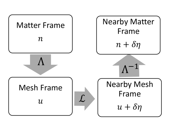
This non-commutation of the frame boosts complicates matters somewhat and one needs to apply all three boosts sequentially, keeping corrections to first order in $\delta\eta$. This procedure is described in Figure 4.1 for mesh expansion corrections to the fluid velocity. If $\mathcal{L}$ commuted with $\Lambda$ to first order in $\delta\eta$, one could apply $\mathcal{L}$ directly to $n$ to obtain the expansion corrections.

For derivatives of quantities in the fluid frame, we need to boost the correction, $\mathcal{L}=\delta\Lambda$, into the fluid frame. Using again Equation 4.8,

$$\Lambda^{\mu\alpha}(u,n)\Lambda^{\nu\beta}(u,n)\delta\Lambda_{\alpha\beta} = \Lambda^{\mu\alpha}\Lambda^{\nu\beta}(n_{\alpha}\eta_{\beta}-\eta_{\alpha}n_{\beta}),$$

$$(\Lambda\Lambda\delta\Lambda)^{\mu\nu} = (2\gamma n^{\mu}-u^{\mu})(\eta^{\nu}+2(u\cdot\eta)n^{\nu}-\frac{u\cdot\eta}{1+\gamma}[u^{\nu}+n^{\nu}])$$ (4.32)

$$-(\eta^{\mu}+2(u\cdot\eta)n^{\mu}-\frac{u\cdot\eta}{1+\gamma}[u^{\mu}+n^{\mu}])(2\gamma n^{\nu}-u^{\nu}).$$

Note that $\Lambda^{\nu\beta}(u,n)$ boosts from the mesh frame to the matter frame and that the boosts are not written in the order of application.

Applying this to the matter frame velocity, we obtain several results

$$(\Lambda\Lambda\delta\Lambda)^{0}_{~{}\alpha}n^{\alpha} = \gamma(u\cdot\eta)-\gamma(u\cdot\eta)=0,$$ (4.33)

$$(\Lambda\Lambda\delta\Lambda)^{x}_{~{}\alpha}n^{\alpha} = -u^{x}(u\cdot\eta)+\frac{\gamma}{1+\gamma}u^{x}(u\cdot\eta)=\frac{-u^{x}}{1+\gamma}u^{z}\delta\eta,$$ (4.34)

$$(\Lambda\Lambda\delta\Lambda)^{z}_{~{}\alpha}n^{\alpha} = -u^{z}(u\cdot\eta)-\gamma\left[\eta^{z}-\frac{u^{z}}{1+\gamma}(u\cdot\eta)\right]=\left[\gamma-\frac{(u^{z})^{2}}{1+\gamma}\right]\delta\eta,$$ (4.35)

and a few results for the shear tensor

$$(\Lambda\Lambda\delta\Lambda)^{x}_{~{}\alpha}\tilde{\pi}^{\alpha\nu} = -u^{x}\delta\eta\tilde{\pi}^{z\nu},$$ (4.36)

$$(\Lambda\Lambda\delta\Lambda)^{z}_{~{}\alpha}\tilde{\pi}^{\alpha\nu} = -(u^{z}\tilde{\pi}^{z\nu}-u_{\alpha}\tilde{\pi}^{\alpha\nu})\delta\eta=(u^{x}\tilde{\pi}^{x\nu}+u^{y}\tilde{\pi}^{y\nu})\delta\eta.$$ (4.37)

Applying the small boost to each index is not necessary as this would produce a second-order correction. As was the case for the collective velocity, these correction factors alter the longitudinal derivatives of the local shear tensor. For example, Equation 4.34 means the longitudinal derivative of the matter frame transverse velocity, $\partial_{\eta}n^{x}$, should be calculated by the finite difference in the longitudinal direction in addition to the mesh factor: $-u^{x}u^{z}/(1+\gamma)$.

4.1.4 Equations of Motion

Since we wish to use the local shear tensor, our derivation of the equations of motion begin in the fluid frame. In this frame, the conservation equations take the form

$$\tilde{\partial_{t}}\epsilon+(\epsilon+P)~{}\tilde{\partial_{i}}n^{i}+\tilde{\pi}^{ij}~{}\tilde{\partial}_{i}n^{j} = 0,$$ (4.38)

$$(\epsilon+P)~{}\tilde{\partial_{t}}n^{i}+\tilde{\pi}^{ij}~{}\tilde{\partial_{t}}n^{j}+\tilde{\partial}_{i}P+\tilde{\partial_{j}}\tilde{\pi}^{ij} = 0,$$ (4.39)

where we have excluded terms that are explicitly zero in this frame. For reasons explained in the following subsection, we expand all time derivatives but leave some spatial derivatives in the form of Equation 4.20. We exclude corrections for bulk viscosity from the conservation equations for simplicity as the corrections alter the pressure but do not add any interesting structure.

Expanding energy conservation in this way produces

$$\gamma\dot{\epsilon}+\frac{(\epsilon+P)u^{i}}{\gamma}\dot{u}^{i}+(u^{i}\tilde{\pi}^{ij})\dot{u}^{j}-\frac{(u^{i}u^{j}\tilde{\pi}^{ij})u^{k}}{\gamma(1+\gamma)}\dot{u}^{k}$$ (4.40)

$$+u^{i}\partial_{i}\epsilon+(\epsilon+P)\partial_{i}u^{i}+\tilde{\pi}^{ij}(\tilde{\partial}_{i}n^{j})^{\prime} = 0$$

where the second term of the first line comes from $\dot{\gamma}$ and final two terms of the first line come from $\tilde{\partial}_{i}n^{j}$.

The same procedure for momentum conservation gives

$$u^{i}c_{s}^{2}\dot{\epsilon}+(\epsilon+P)\gamma\dot{u}^{i}-\frac{(\epsilon+P)u^{i}u^{j}}{1+\gamma}\dot{u}^{j}+\gamma\tilde{\pi}^{ij}\dot{u}^{j}$$ (4.41)

$$+\frac{u^{k}}{1+\gamma}\left[u^{i}\tilde{\pi}^{kj}-2\tilde{\pi}^{ik}u^{j}\right]\dot{u}^{j}+(\gamma-1)\tilde{\pi}^{ij}\dot{u}^{j}+u^{j}\dot{\tilde{\pi}}^{ij}$$

$$+(\epsilon+P)(\tilde{\partial}_{t}n^{i})^{\prime}+\tilde{\pi}^{ij}(\tilde{\partial}_{t}n^{j})^{\prime}+\partial_{i}P+\frac{u^{i}u^{k}}{1+\gamma}\partial_{k}P+(\tilde{\partial}_{j}\tilde{\pi}^{ij})^{\prime} = 0.$$

where $(\tilde{\partial}_{j}\tilde{\pi}^{ij})^{\prime}$ includes the effects of boosting the derivative and the effects of the collective velocity on the shear tensor in nearby fluid cells. This form of the momentum conservation equations include time derivatives of the local shear tensor, which are not among the integrated variables. Conversion of these to time derivatives of $\alpha_{i}$ makes the equations even more difficult to parse, and the conversion takes the simple form

$$\dot{\pi}^{ij}=\partial_{\tau}\left[\sigma_{\eta}P_{ijk}\alpha_{k}\right]=P_{ijk}\alpha_{k}\frac{\partial\sigma_{\eta}}{\partial\epsilon}\dot{\epsilon}+\sigma_{\eta}P_{ijk}\dot{\alpha_{k}}$$ (4.42)

where $P_{ijk}$ projects out the correct $\alpha_{k}$’s according to the inverse mapping corresponding to Equation 4.3.

The remaining equations of motion are the relaxation equations for the shear tensor. We rewrite Equation 2.20 in terms of the scaled, projected moments of the shear tensor,

$$\tau_{\pi}\tilde{\partial}_{t}\alpha_{i}=-\alpha_{i}-\frac{\eta}{\sigma_{\eta}}\omega_{i}$$ (4.43)

where $\omega_{i}$ is the projection of the Navier-Stokes velocity gradients described in Equation 4.5. As an example, for the first projected shear stress element this is

$$\gamma\dot{\alpha}_{1}+u^{i}\partial_{i}\alpha_{1}+\frac{\alpha_{1}}{\tau_{\pi}}=\frac{-\eta}{\sigma_{\eta}\tau_{\pi}}(\tilde{\partial}_{x}n^{x}-\tilde{\partial}_{y}n^{y}).$$ (4.44)

Expanding this to the form of Eq. 4.51 yields

$$\gamma\dot{\alpha}_{1} - \frac{2}{(1+\gamma)\sigma_{\eta}}\left[\left(u^{x}\tilde{\pi}^{xj}-u^{y}\tilde{\pi}^{yj}\right)\dot{u}^{j}-u^{j}\tilde{\pi}^{jx}\dot{u}^{x}+u^{j}\tilde{\pi}^{jy}\dot{u}^{y}\right]$$

$$+ \frac{\eta}{\sigma_{\eta}\tau_{\pi}}\left((u^{x}\dot{u}^{x}-u^{y}\dot{u}^{y})-(u_{x}^{2}-u_{y}^{2})\frac{u^{k}\dot{u}^{k}}{\gamma(1+\gamma)}\right),$$

$$= -u^{i}\partial_{i}\alpha_{1}-\frac{\eta}{\sigma_{\eta}\tau_{\pi}}[(\tilde{\partial}_{x}n^{x})^{\prime}-(\tilde{\partial}_{y}n^{y})^{\prime}],$$

where $\partial_{i}\alpha_{1}$ still contains corrections due to velocity gradients.

4.1.5 Time Integration

As stated before, the algorithm is written on a fixed grid in the expanding coordinate system. The integration variables, denoted $V_{i}$ are the natural logarithm of the energy density – $\varepsilon=\ln\epsilon$, the collective velocity relative to the expansion – $\vec{u}$, and the scaled, projected local shear tensor – $\alpha_{i}$ as given by Equation 4.4.

The choice of the logarithm of the energy density is motivated by the shape of the fireball. Models that we consider for the initial energy density tend to have tails that are either Gaussian or exponential. Taking the logarithm means that second-order finite difference derivatives will be exact for such profiles.

Furthermore, the structure of the source term from the Bjorken expansion suggests that one should not use linear proper time at early times. Consider a (0+1)-dimensional system under going a Bjorken expansion. For such a system, the evolution of the energy density is given by

$$\frac{d\epsilon}{d\tau}=\frac{-(\epsilon+P)}{\tau}.$$ (4.46)

If one used a first order upwind solver (often called Euler integration) for this application, the source term would always be too large since the proper time would be smaller when the term was evaluated. This error goes like $e^{-\tau}$ and was found to produce integrated errors on the order of 1% in simple situations whereas the final code produces total integrated errors on the order of 0.1% for more complex situations.

These simple integration errors suggest that one should integrate in the logarithm of proper time, $x=\ln{\tau}$. This changes the energy density evolution to

$$d\epsilon=-(\epsilon+P)\frac{d\tau}{\tau}=-(\epsilon+P)dx.$$ (4.47)

While this reduces integration errors at small times, for a fixed $\Delta x$ the size of the proper time steps grows without bound. This introduces numerical instability by violation of the Courant condition. A pleasant compromise defines $x=\ln\sinh\tau$, which causes the time integration to proceed slowly at first getting the Bjorken corrections right but limits the steps to a fixed maximum size. Results for the equations of motion will ignore this distinction.

Spatial derivatives are evaluated using centered second-order finite differences of the integration variables

$$\partial_{j}V_{i}(x^{\mu})=\frac{V_{i}(x^{\mu}+\triangle x^{j})-V_{i}(x^{\mu}-\triangle x^{j})}{2|\triangle x^{j}|},$$ (4.48)

which assumes that the $V_{i}$ is locally parabolic. The hot region in a heavy ion collision obviously has no hard boundary to couple to, instead we must deal with coupling to the vacuum at the edges of the computational region. There, we use an asymmetric second-order finite difference

$$\partial_{j}V_{i}(x^{\mu})=\frac{3V_{i}(x^{\mu})-4V_{i}(x^{\mu}-\triangle x^{j})+V_{i}(x^{\mu}-2\triangle x^{j})}{2|\triangle x^{j}|},$$ (4.49)

for the positive $x_{j}$ boundary and the equivalent for the negative $x_{j}$ boundary. Equations 4.48 and 4.49 produce the same result if the function is exactly parabolic in the region $x^{\mu}-2\triangle x_{j}<x^{\mu}<x^{\mu}+2\triangle x_{j}$. Using the same order derivatives at the boundary proved important for modeling systems whose tails were not purely exponential.

Time integration is done simultaneously for all integration variables using the second-order Runge-Kutta method, sometimes called the predictor-corrector method. This method uses spatial derivatives at a fixed proper time to compute proper time derivatives at that time. These are used to move the system forward by a half-step in time by finite difference and the results are stored in a separate mesh. Spatial derivatives computed are then computed on the advanced mesh, from which time derivatives are computed. These time derivatives are used to advance the original mesh a full step. For a one-variable integration, this amounts to

$$V_{i}(t+\triangle t/2) = V_{i}(t)+\frac{\triangle t}{2}\left.\frac{\partial V_{i}}{\partial t}\right|_{t},$$

$$V_{i}(t+\triangle t) = V_{i}(t)+\triangle t\left.\frac{\partial V_{i}}{\partial t}\right|_{t+\triangle t/2}.$$ (4.50)

This procedure is repeated until all of the fluid cells are below the freezeout temperature.

The equations of motion are coupled in the sense that the continuity equation contains time derivatives of the energy density and the velocities though not the shear tensor. Decoupling the equations is tedious algebraically and it is not clear that such a procedure would be computationally beneficial. Instead, we find the time derivatives on a mesh by considering the coefficients to all the time derivatives as a matrix equation

$$C_{ij}(V_{m})\dot{V}_{i}=b_{j}(\partial_{m}V_{n},V_{i})$$ (4.51)

where $C_{ij}$ is the coefficient matrix that depends on the coordinates and integration variables but $b_{j}$ also depends on their derivatives. $C_{ij}$ can be inverted for each fluid cell to find the time derivatives. In this form, the coefficient matrix is invertible unless the viscous corrections are larger than the energy density where Israel-Stewart theory would not be valid in any event. Such situations do not seem to arise unless the system begins in such a condition, though this happens frequently if the system begins with viscous corrections from the Navier-Stokes theory which will be discussed later.

The code is also designed to run in modes that reduce the integration region using system symmetries that are frequently present for smooth initial conditions. In many cases the gradients of the energy density can be aligned with the coordinate axes and have reflective symmetry with respect to the coordinate planes. This allows one to integrate a single octant of configuration space. Since the velocity vector arises from the gradient of the energy density, it is anti-symmetric in the sense that $u^{x}(\delta x)=-u^{x}(-\delta x)$ but $u^{x}(\delta y)=u^{x}(-\delta y)$. The shear tensor gets it symmetry structure from the velocity gradients that produce it. This means that on-diagonal components are even in all coordinates, and off-diagonal components are odd in their coordinates and even otherwise, which we summarize as

$$\pi^{xx}(\delta\vec{r})=\pi^{xx}(-\delta\vec{r});~{}~{}\pi^{xy}(\delta x)=-\pi^{xy}(-\delta x);~{}~{}\pi^{xy}(\delta z)=\pi^{xy}(-\delta z).$$ (4.52)

This could be violated if the initial conditions for the shear tensor are not proportional to velocity or density gradients, though the source of such conditions is not immediately clear.

4.2 Verification of Hydrodynamic Algorithm

This section focuses on efforts to verify that the code solves the correct set of equations and solves them to sufficient accuracy for application to heavy ion collisions. The general approach is to confirm that the ideal hydrodynamics algorithm conserves entropy, that the viscous hydrodynamics algorithm conserves $T^{00}$, that results from lower dimensional codes are qualitatively reproduced.

4.2.1 Conserved Quantities

As discussed in Chapter 2, ideal hydrodynamics locally conserves entropy. For an infinite system, the volume integral of the entropy density over the whole space would be a constant. Since most hydrodynamic algorithms are unstable in regions where the velocity gradients are large and the energy density is small, the integration region is cutoff at temperatures around 50 MeV. Over the length of the calculation, the entropy flux from the integration region is not negligible at the level of conservation that we hope to achieve. As such, it must be calculated in order to ensure proper conservation.

In the $\eta$-$\tau$ coordinate system, there is an additional term due to the work done by the expanding fluid cell:

$$0 = \int d^{4}x\tau d_{\mu}s^{\mu}=\int d^{4}x\tau\partial_{\mu}s^{\mu}+\int d^{4}xs\gamma=\int d\tau dxdyd\eta\left[\partial_{\tau}(\tau\gamma s)+\tau\vec{\nabla}\cdot(\vec{u}s)\right],$$

$$C = \int dxdyd\eta(\tau\gamma s)+\int\tau d\tau\int s\vec{u}\cdot d\vec{A},$$ (4.53)

where $C$ is a constant, $d\vec{A}$ is a surface element, and the velocity is relative to the expanding mesh. Note that the expansion of the fluid cell has been incorporated into the first integral which is over the volume at fixed proper time. At each time step, the integral over all cells and the flux integral over the surface are calculated. Time integrals are evaluated via second order Runge-Kutta, using the surface integrals evaluated on the intermediate grid. The result is compared to the same integral done in the first step. For typical ideal calculations, the entropy conservation integral was found to be conserved at the level of 0.1%. The importance of changes to the integration scheme as described above improved this conservation by an order of magnitude for calculations beginning at proper times of $\tau=0.1$ fm/c, though this is earlier than typical calculations.

Furthermore, viscous hydrodynamic calculations were checked to ensure that entropy increases monotonically throughout. More satisfying would be to check a conserved quantity and a useful choice for the viscous case is $T^{00}$, since $T^{0i}$ conservation can be verified by symmetry. We provide the same calculation as for entropy conservation

$$0 = \displaystyle\int d^{4}xd_{\mu}T^{\mu 0}=\displaystyle\int d\tau d\eta dxdy\left[\partial_{\tau}T^{00}+\partial_{i}T^{0i}+\frac{T^{00}+T^{zz}}{\tau}\right],$$

$$C = \displaystyle\int T^{00}\tau d\eta dxdy+\displaystyle\int d\tau\left[\displaystyle\oint T^{0i}ds^{i}+\displaystyle\int T^{zz}d\eta dxdy\right],$$ (4.54)

where $T^{0i}ds^{i}$ is the outgoing momentum flux. Here the extra terms due to the expansion cannot be completely avoided and an integral over all time and space must be tracked. This integral tends to be about 25% of the total by the end of calculation. Still we find that this integral is conserved at the 0.1% level for typical initial conditions and cell densities.

4.2.2 Comparison to Known Results

The equations of motion for second-order viscous hydrodynamics are quite complex and verifying that the code solves the correct set of equations is not trivial. Since the conservation equations involve first-order time derivatives and first-order spatial derivatives, one natural approach to find an analytic solution for verification is to consider an exponential dependence of the density for a static system

$$\epsilon=\epsilon_{0}\cdot e^{-x/R},~{}~{}~{}~{}~{}\vec{u}=0,$$ (4.55)

where $\epsilon_{0}$ and $R$ are constants. For verification purposes we arbitrarily take $R=3$ fm; and the initial energy density, $\epsilon_{0}$, was taken at many values to ensure numerical accuracy for a practical range of values, but presented results will be normalized by this factor. We will investigate Such a system has infinite energy and is therefore not physical except locally, but we emphasize that this is a test case. The collective velocity begins at the same value everywhere and the absence of velocity gradients proves a stable point, which will be clear when we arrive at the equations of motion for the velocity and energy density. A constant speed of sound is a necessary condition for this behavior.

For an ideal system, there are only two equations to be found - for the velocity and energy density - which come from the continuity equations and one Euler equation. We begin by investigating the case without a longitudinal expansion and return to that such conditions later. From energy conservation, we obtain

$$\partial_{\mu}T^{\mu 0} = 0,$$

$$(1+c_{s}^{2})\gamma u\frac{\epsilon}{R} = 2\epsilon(1+c_{s}^{2})u\dot{u}+[\gamma^{2}+c_{s}^{2}(\gamma^{2}-1)]\dot{\epsilon},$$ (4.56)

and from momentum conservation,

$$\partial_{\mu}T^{\mu x} = 0,$$

$$\left[u^{2}(1+c_{s}^{2})-c_{s}^{2}\right]\frac{\epsilon}{R} = \frac{(1+c_{s}^{2})\epsilon}{\gamma}[u^{2}+\gamma^{2}]\dot{u}+(1+c_{s}^{2})\gamma u\dot{\epsilon}.$$ (4.57)

Figure 4.2: (color online) The collective velocity at all points for a exponential energy density profile with no Bjorken expansion (blue squares), a transverse profile with Bjorken expansion (red stars), and a longitudinal profile with Bjorken expansion (green triangles). In each case the velocity calculated by the full code agrees with the correct value.

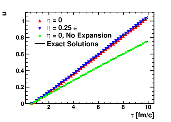
The system of Equations 4.56 and 4.57 can be solved for $\dot{\epsilon}/\epsilon$ and $\dot{u}$, where the former is only possible due to the choice of the density gradient as proportional to the density. This separability proves that the absence of velocity gradients is a stable condition for this initial condition. The equation for the velocity is

$$\dot{u}=\frac{\gamma}{\gamma^{2}-c_{s}^{2}u^{2}}\cdot\frac{c_{s}^{2}}{R(1+c_{s}^{2})},$$ (4.58)

where we have used the constant speed of sound. For early times when the collective velocity is small, the solution to Eq. 4.58 is linear,

$$u(t)\propto\frac{c_{s}^{2}}{R(1+c_{s}^{2})}t.$$ (4.59)

While Eq. 4.58 is exactly integrable, the solution is not invertible

$$\frac{c_{s}^{2}}{R(1+c_{s}^{2})}\int dt = \int du~{}~{}\frac{1+u^{2}(1-c_{s}^{2})}{\sqrt{1+u^{2}}},$$ (4.60)

$$\frac{c_{s}^{2}}{R(1+c_{s}^{2})}t = \frac{1}{2}\left[(1+c_{s}^{2})\sinh^{-1}(u)+(1-c_{s}^{2})u\sqrt{u^{2}+1}\right]$$ (4.61)

which limits its utility. Figure 4.2 shows that the agreement of the code with this solution.

The addition of the Bjorken expansion does not lead to an analytic solution, but the computation provides a stricter test on the code and can be done with a much less complex numerical routine. The conservation equations are modified as follows: for energy conservation

$$\partial_{\mu}T^{\mu 0}+(T^{00}+T^{zz})/\tau = 0,$$

$$(1+c_{s}^{2})\gamma u\frac{\epsilon}{R}+\gamma^{2}(\epsilon+P)/\tau = 2\epsilon(1+c_{s}^{2})u\dot{u}+[\gamma^{2}+c_{s}^{2}(\gamma^{2}-1)]\dot{\epsilon},$$ (4.62)

and for momentum conservation

$$\partial_{\mu}T^{\mu x}+T^{0x}/\tau = 0,$$

$$\left[u^{2}(1+c_{s}^{2})-c_{s}^{2}\right]\frac{\epsilon}{R}+\frac{u\gamma(1+c_{s}^{2})\epsilon}{\tau} = \frac{(1+c_{s}^{2})\epsilon}{\gamma}[u^{2}+\gamma^{2}]\dot{u}+(1+c_{s}^{2})\gamma u\dot{\epsilon}.$$ (4.63)

Solving these equations for $\dot{u}$ yields

$$\dot{u}=\frac{\gamma c_{s}^{2}}{\gamma^{2}-c_{s}^{2}u^{2}}\left[\frac{\gamma u}{\tau}+\frac{1}{R(1+c_{s}^{2})}\right],$$ (4.64)

where the first term in the brackets comes from the Bjorken expansion and differentiates it from Eq. 4.58. The inseparability of the equation makes the prospects of an analytic solution unlikely, but the expression can be used for comparison with a simple and easily verified numerical code. Comparison to the larger code again validates the larger (3+1)-dimensional code which is again shown in Figure 4.2. Note that the presence of the Bjorken expansion actually significantly increases the transverse expansion rate. Shear viscosity will further increase the transverse expansion rate as viscosity tends to resist the asymmetric expansion inherent to the Bjorken initial condition.

Also shown in Figure 4.2 is the same result if the exponential distribution is in the longitudinal direction where $\epsilon\propto e^{\eta/\sigma}$, which is also reproduced. While in the transverse case the expansion due to the infinite exponential profile continues forever, in the longitudinal case, the expansion of the mesh means that the effective gradients get weaker over time. The inclusion of the mesh expansion can be accounted for by making the substitution $R\rightarrow\tau\sigma$ in the final results of Eq. 4.64, which comes from correcting the spatial derivative $\partial_{z}\rightarrow\tau^{-1}\partial_{\eta}$.

Figure 4.3: (color online) The ratio of the energy density to its initial value for a exponential energy density profile with a Bjorken expansion in the ideal case (red squares) and with shear viscosity equal to one quarter of the energy density. In either case the calculation produces the correct energy density.

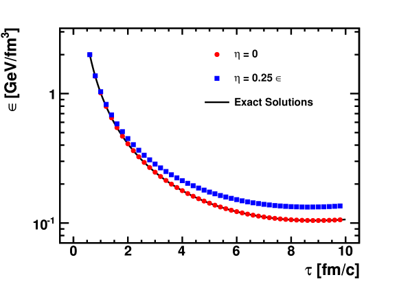
The equations for the collective velocity are easy to work with as they involve only the velocity itself. For the energy density, the logarithmic time derivative can be written as a function of the collective velocity. For the case without the Bjorken expansion, one simply uses the result in Eq. 4.58 along with Eq. 4.56 or 4.57. This results in

$$\frac{\dot{\epsilon}}{\epsilon}=\frac{\gamma u(1-c_{s}^{2})}{R(u^{2}(1-c_{s}^{2})+1)}.$$ (4.65)

While this expression is not so pleasing, it can be integrated to obtain $\epsilon(u)$ using a change of variables:

$$\int\frac{d\epsilon}{\epsilon} = \int du\frac{dt}{du}\frac{d\epsilon}{dt},$$

$$\ln\left[\frac{\epsilon}{\epsilon_{0}}\right] = \int_{0}^{u}du~{}~{}\frac{R(1+c_{s}^{2})(u^{2}(1-c_{s}^{2})+1)}{\gamma c_{s}^{2}}\cdot\frac{u\gamma(1-c_{s}^{2})}{R(u^{2}(1-c_{s}^{2})+1)},$$

$$= \frac{1-c_{s}^{4}}{c_{s}^{2}}\int_{0}^{u}u~{}~{}du,$$

$$\ln\left[\frac{\epsilon}{\epsilon_{0}}\right] = \frac{1-c_{s}^{4}}{2c_{s}^{2}}\cdot u^{2},$$

$$\epsilon = \epsilon_{0}\cdot\exp\left[\frac{1-c_{s}^{4}}{2c_{s}^{2}}u^{2}\right].$$ (4.66)

To the extent that $u$ is linear for small $t$, $\epsilon$ grows like $e^{t^{2}}$. Again we emphasize that this is not intended to be a physical solution and mainly the super-exponential growth is due to the original exponential density distribution everywhere. Also note that while this expression appears not to depend on the length scale from the density distribution, but this information enters through the velocity. Eq. 4.66 was also used to verify the full code.

The Bjorken expansion can be added again. The result can be arrived at by using the result for the time derivative of the velocity with either conservation equation, or by returning to the conservation equations and resolving. The result of either is

$$\frac{\dot{\epsilon}}{\epsilon}=\frac{\gamma}{u^{2}(1-c_{s}^{2})+1}\cdot\left[\frac{(1-c_{s}^{2})u}{R}-\frac{(1+c_{s}^{2})\gamma}{\tau}\right].$$ (4.67)

An analytic solution to this equation was not attempted, but the equation was numerically integrated using a small code and again confirmed the full code shown in Figure 4.3 Note that at large times the expansion due to the infinite exponential initial condition eventually overcomes the Bjorken expansion. However, the lifetime of the matter created in $\sqrt{s}=200$ GeV Au+Au collisions tends to be less than 10 fm/c and up until around this time the evolution of the energy density is dominated by the Bjorken expansion even where the density gradients are significant. Therefore, we expect the lifetime of the system to be roughly independent of the transverse details.

The above scenarios demonstrate that the conservation equations are being correctly solved in the absence of shear viscosity. Adding shear viscosity would tend to spoil the constancy of the collective velocity simply by introducing a new scale to the problem. However if the shear viscosity also scaled with the energy density and the relaxation time was a constant the scaling solution would not be broken. This violates the Second Law of Thermodynamics and is unphysical based solely on units, but it is useful for testing purposes.

Figure 4.4: (color online) Viscous corrections to the pressure along each axis for the transverse exponential test of the hydrodynamics code for a viscous system undergoing a Bjorken expansion. This demonstrates that TRISH reproduces analytic results for viscous hydrodynamics as well as ideal hydrodynamics

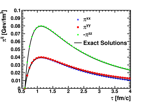
Deriving the equations of motion for the shear tensor in addition to the conservation equations is a bit tedious and not particularly enlightening. For completeness, the equations of motion to be integrated are

$$\gamma\dot{\epsilon}+\frac{u}{\gamma}\left(\epsilon+P+\frac{\pi^{xx}}{\gamma^{2}}\right)\dot{u} = \frac{u\epsilon}{R}-\frac{\gamma}{\tau}\left(\epsilon+P+\pi^{zz}\right),$$ (4.68)

$$\gamma uc_{s}^{2}\dot{\epsilon}+\gamma\left(\epsilon+P+\frac{1-u^{2}}{\gamma^{4}}\pi^{xx}\right)\dot{u}+\frac{u}{\gamma}\dot{\pi}^{xx} = \frac{c_{s}^{2}\gamma^{2}\epsilon+\pi^{xx}}{R}+\frac{u}{\gamma\tau}\left(\gamma^{2}\pi^{zz}-\pi^{xx}\right),$$

$$\frac{2u}{3}\left(\frac{2\gamma\eta}{\tau_{\pi}}-\frac{\pi^{xx}}{\gamma}\right)\dot{u}+\gamma\dot{\pi}^{xx} = \frac{-\pi^{xx}}{\tau_{\pi}}+\frac{u\pi^{xx}}{R}+\frac{2\gamma}{3\tau}\left(\frac{\gamma^{2}\eta}{\tau_{\pi}}-2\pi^{xx}\right),$$

$$\frac{2u}{3\gamma}\left(2\pi^{zz}-\frac{\eta}{\tau_{\pi}}\right)\dot{u}+\gamma\dot{\pi}^{zz} = \frac{-\pi^{zz}}{\tau_{\pi}}+\frac{u\pi^{zz}}{R}-\frac{4\gamma}{3\tau}\left(\frac{\eta}{\tau_{\pi}}+\pi^{zz}\right).$$

This system of equations has the structure of the full set of equations in that it contains the dependence of time derivatives of the shear components on the conservation equations and vice versa. This means that this test case would identify errors in the matrix inversion procedure. In addition, frequently terms are not expressed in this set of equations in the same way that they are expressed in the full code and a large fraction of terms are represented and checked.

The results of the full code and a small test program are shown in Figure 4.2 for collective velocity, in Figure 4.3 for the energy density, and in Figure 4.4 for components of the shear tensor, each in the viscous case. Only two components of the shear tensor need to be calculated due to orthogonality with the collective velocity and tracelessness of the shear tensor. The test code is written to integrate only $\pi^{xx}$ and $\pi^{zz}$, whereas the full code integrates $\alpha_{i}$ meaning that some numerical effects are different between the two codes. These normalized deviations were found to be on the order of $10^{-4}$ or less.

Figure 4.5: (color online) The location of the $T=130$ MeV isotherm along the line $y=0$ for comparison with another numerical code, where the ideal results have been reflected $\tau\rightarrow-\tau$ for the case, $\eta/s=0$. Comparison shows that the hydrodynamic codes produce the same freezeout surface for the case of zero or small shear viscosity.

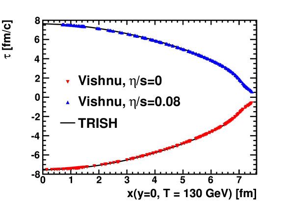
Comparisons for more realistic conditions were made in the interest of validation. Particularly of interest were calculations of the motion of a constant temperature surface, as these are the principle output of the hydrodynamic calculations. The chosen initial conditions were energy density scaled to the number of wounded nucleons (see Chapter 5), zero initial collective flow, and shear corrections as given by Navier-Stokes for viscous simulations. The equation of state is from a massless gas, and the shear viscosity was scaled to the entropy density.

Numerical results for the initial conditions were provided by the TECHQM collaboration for code verification. These codes are restricted to boost invariant problems and so the following comparisons will be done for boost invariant initial conditions. For the ideal case, the initial conditions were matched exactly. In the viscous case, the choice of Navier-Stokes shear corrections has the problem that the corrections become much larger than the pressure at low temperature, because the shear viscosity is proportional to $T^{3}$ and the pressure is proportional to $T^{4}$, so the ratio $\eta/P\propto T^{-1}$ diverges at low temperature. While physically this is not concerning as the simulation is only valid if the motion of the surface is not strongly influenced by the details of the evolution at temperatures much lower than the freezeout temperature, large viscous corrections make hydrodynamic calculations unstable.

The TECHQM collaboration chose to unphysically compensate by making the shear viscosity decrease at large distances from the center of the hot region. TRISH was instead run with the initial shear corrections proportional to the pressure at all temperatures with the corrections in the center of the calculation roughly the same as the Navier-Stokes value. It has been found that this does not significantly affect observables in general, and in this case we find that it has little effect on the hydrodynamics.

The motion of the point of constant temperature ($T=130$ MeV) along the line $\eta=y=0$ as a function of the proper time is shown in Figure 4.5. The differences in integration strategy mean that the calculations make predictions at different times, making a differential comparison reliant on interpolation strategy. Still, we found qualitative agreement between the codes in both the ideal and viscous cases. This includes the general feature that viscosity increases the transverse pressure at early times, which causes the temperature isosurface to remain at larger distances from the center at moderate times, before collapsing more suddenly at roughly the same final time.

Figure 4.6: (color online) The sum of the transverse shear corrections to the pressure as a function of proper time for the isotherm $T=130$ MeV and along the line $y=\eta=0$. While the initial value differs due to scaling with the pressure, the corrections have the same general behavior.

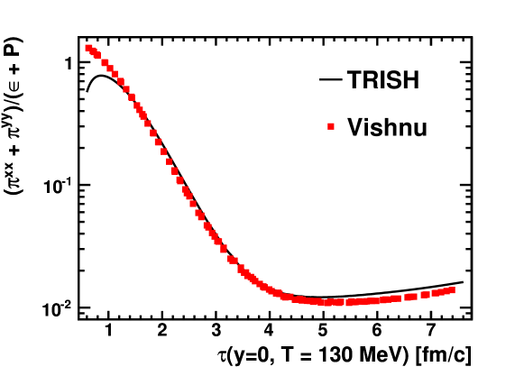
In addition to the evolution of the freezeout surface, the shear correction to the phase space density has a significant effect on emitted particle momentum distributions. This is most notable in elliptic flow which is reduced by the correction to the phase space density as described in Equation 2.31. To confirm that our predictions for the shear correction at the freezeout surface Figure 4.6 shows its evolution as a function of proper time along the line $y=\eta=0$. The initial value of the correction is smaller for our calculation due to the choice of initial state but the two solutions converge rapidly to the same behavior. While deviations at larger times are on the order to 10%, it is not clear if this is due to differences in the initial state or differences in integration scheme.

4.3 Liquid-Gas Coupling

4.3.1 Particle Creation

The low temperature regions of the calculation cannot be calculated as a liquid even within the Israel-Stewart framework. In these regions, the mean free paths of the particles become larger than the size of the system and local kinetic equilibrium can no longer be maintained. Furthermore, differences between particle species become important as the pions begin to flow faster and cool slower than heavier particles such as protons. Other groups have attempted to address this by tracking fluctuations of baryon number and other conserved charges and their associated fugacities below some chemical freezeout temperature, while assuming that ideal hydrodynamics still governs the kinetic behavior until some lower temperature. This approach is motivated by the data which display softer spectra than the particle ratios would suggest, but strain credibility by assuming local equilibration with long mean free paths and low Reynolds numbers.

A more satisfactory approach is to couple the hydrodynamic calculation to a gas calculation that treats particles as the important degrees of freedom. In principle, a simulation of both the fluid and the gas phases could proceed simultaneously with the fluid receiving information about the pressure in the gas and the gas receiving information about the emission of particles from the fluid. In practice, this is a very demanding calculation and the fluid likely does a good job of approximating the motion of the gas for temperatures near to the phase transition assuming the equation of state is consistent. The reverse is also of concern; if this temperature is chosen to be too high, the hadrons cannot be treated as independent, incoherent objects and corrections akin to the classical finite volume correction become important. Fortunately for temperatures around $140\leq T\leq 165$MeV the two descriptions mesh nicely. [53]

In general, the goal is to generate a distribution of particles such that the stress-energy tensor is the same in the freezing fluid cell as it is for the particles that are now in that same volume. In the gas phase, the stress-energy tensor is given by

$$T^{ij}=\displaystyle\sum\limits_{s}\displaystyle\int\frac{d^{3}p}{(2\pi)^{3}}\frac{p^{i}p^{j}}{E(\vec{p})}f_{s}(\vec{p}),$$ (4.69)

where $s$ indexes the particle species. While this is at least a well-defined task if the phase space density is given, in viscous hydrodynamics the phase space density is altered by the presence of shear viscosity. As discussed in Chapter 2, viscous corrections are related to the distortion of the phase space density. In Equation 2.31, we took the relationship of the shear tensor to the phase space distortion as the Grad ansatz, which has the general form

$$f(p^{\mu},r^{\nu})=f_{\text{eq}}(p^{\mu},r^{\nu})\left[1+C(p)p_{\alpha}p_{\beta}\pi^{\alpha\beta}_{(s)}\right],$$ (4.70)

where the momentum dependence of the correction coefficient, C(p), may be different for different species. This form has the difficulty that the correction term can become arbitrarily large and certainly will do so at large momentum leading to negative phase space density [7, 54, 55].

An alternative approach [53] would be to evaluate the equilibrium phase space density at an altered momentum by shifting linearly in the form

$$p_{i}=p_{i}^{\prime}+A\tilde{\pi}^{ij}p_{j}^{\prime},$$ (4.71)

where A is a coefficient to be determined, $\tilde{\pi}^{ij}$ is the shear correction in the fluid frame. This allows one to generate particles according to a static thermal distribution and then adjust the momentum to reproduce the local shear tensor before applying the boost from the fluid frame to the lab frame.

This linear form for the correction can be understood in terms of the Navier-Stokes theory where $\tilde{\pi}^{ij}$ is the velocity gradient. Given that viscous hydrodynamics allows for a non-zero mean free path ($\Delta r$) and collision time ($\Delta t$), particles observed locally have originated nearby. Then the momentum observed locally is given by

$$p_{i}=p_{i}^{\prime}-E\Delta v_{i}=p_{i}^{\prime}-E\partial_{j}v_{i}\frac{p_{j}\Delta t}{E}=p_{i}^{\prime}-\Delta t\partial_{j}v_{i}p_{j}^{\prime},$$ (4.72)

where the velocity gradients are to be evaluated in the fluid frame. More general considerations based on requiring fixed energy and particle densities show that this rough argument holds well and the general form should be

$$p_{i}=p_{i}^{\prime}+\lambda_{ij}p_{j}^{\prime}=p_{i}^{\prime}+\frac{\Delta t}{2\eta}\tilde{\pi}_{ij}p_{j}^{\prime}.$$ (4.73)

In principle, this procedure can be done separately for each particle species, the result of which would be that the pions receive larger phase space corrections than the protons though this is not done at present. Furthermore, $\Delta t$ in Equation 4.73 could be different for each particle species or could depend on momentum.

These results allow one to calculate the phase space density. Combining this with information about the volume elements comprising the freezeout hypersurface, $d\Sigma^{\mu}$, one generates particles according to the Cooper-Frye prescription [56]

$$dN=\frac{f(p\cdot u)d^{3}p}{(2\pi)^{3}E(p)}(p_{\nu}d\Sigma^{\nu})\Theta(p_{\nu}d\Sigma^{\nu}).$$ (4.74)

The direction of $d\Sigma^{\mu}$ is orthogonal to the breakup surface. It points in the time direction for sudden breakup and in the spatial direction for emission from a static shock front. Discussion of calculating the hypersurface elements follows in Section 5.2, but it suffices to understand that the vector points outward, from higher energy density to lower, and has length proportional to the volume of the fluid element undergoing the transition to gas. The step function, $\Theta(p\cdot d\Sigma)$, ensures that we generate only particles that are emitted from the surface rather than particles that are moving further into the fluid. The corollary to this point is that particles within the cascade that move inside of the freezeout surface should be removed from that calculation. For 4d calculations determining surface collisions becomes rather expensive, and for 2d calculations it was found that roughly 1% of the particles actually re-enter the surface due to a combination of significant radial and the rapid shrinking of the hot region. Absorbed particles could be a significantly large effect with fluctuating initial conditions and a more thoughtful consideration in the gas phase would be needed.

To conclude, we summarize the methodology. One first calculates the total number of particles to be emitted by the surface using only the surface volume, temperature and chemical potentials. For each particle, one randomly selects a momentum from a static thermal distribution, which is then scaled to reproduce the stress-energy tensor via 4.73. The momentum is then boosted from the fluid frame to the lab frame. In this frame, one can determine whether the momentum is into or out of the surface by keep or reject Monte Carlo with keep probability $p_{\mu}d\Sigma^{\mu}/(E|d\Sigma|)$. This set of particles are then treated with the gas model.

4.3.2 Surface Finding

While the hydrodynamic calculation extends to rather low temperatures, the model uses the low temperature evolution only as a proxy for the evolution of the gas phase. The output of the hydrodynamic module is in fact the evolution of the boundary between the liquid and gas phases, which is taken to be a temperature isosurface, in terms of the hypersurface vector $d\Sigma^{\mu}$ which characterizes the location and orientation. Generally the strategy [7] is to break the surface into tetrahedra embedded in the four-dimensional space. For each tetrahedron, the surface vector is proportional to the generalized cross-product of the three four-vectors from one vertex to the other three:

$$d\Sigma^{\mu}=(1/6)g^{\mu\nu}\epsilon_{\nu\alpha\beta\gamma}x_{1}^{\alpha}x_{2}^{\beta}x_{3}^{\gamma}$$ (4.75)

where $\epsilon_{\nu\alpha\beta\gamma}$ is the totally anti-symmetric tensor. This only defines $d\Sigma^{\mu}$ up to a sign and one must ensure that the vector points outward. The simplest cases of Equation 4.75 are when the tetrahedron’s vectors are along the coordinate axes. For instance, if the tetrahedron lies along the spatial axes, then the surface vector points in the temporal direction. This means that the surface is collapsing rapidly in time as would happen near the end of the collision when many fluid elements freezeout simultaneously. In contrast, if one of the elements is exactly along the time axis and the other two along spatial axes, the surface is static in time and emission happens outward along the final spatial direction.

The hydrodynamic equations of motion are evaluated on a fixed grid in configuration space in the moving coordinate system described in previous chapters. This means that the mesh is made up of hypercubes that intersect the temperature isosurface. Determining that the isosurface passes through a given hypercube is not difficult – if there is at least one corner above and at least one below the freezeout temperature, then the surface passes through this cube. Rather all of the subtlety is in determining the orientation and volume of surface within the hypercube. This problem has been studied in great detail in three dimensions for the purpose of surface finding for graphical applications [57]. On of the most famous and successful algorithms is called Marching Cubes, which uses the cubic symmetry of the mesh and breaks down all possible combinations of vertices inside and outside the surface exhaustively.

Figure 4.7: Shows the freezeout surface passing through two adjacent cubes in a three dimensional space. The top figure demonstrates double counting resulting from assuming that the surface is a single sheet in each cube. The middle panel demonstrates the possibility that the surface could develop a hole, while the bottom panel shows a consistent solution as determined by the Marching Cubes algorithm.[7]

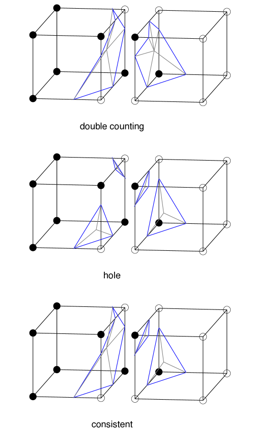
In three-dimensions, Marching Cubes produces a triangulation of the surface within each cube. One of the key difficulties of resolving each cube individually is the relationship between surfaces in adjacent cubes. For instance, in the two-dimensional case (a square) when opposite corners are on one-side of the surface, there are two configurations of the lines that would make up the surface – one with the center above the surface and one below. A self-consistent approach to determining which of these configurations is to be used is required. In this case, whether the center of the face is inside or outside the surface is determined by the average of all four values, though more complicated approaches exist [7] . Failure to account for this possibility leads to significant overlaps or holes in the surface even for relatively simple configurations, for instance Figure 4.7 shows possible errors and a self-consistent solution for adjacent cubes. The difficulty here is that the surface should have two pieces in the right cube and one piece in the left cube. Use of the average along that cube face allows the algorithm to determine that the center is on the white side of the surface, and make the correct choice of tilings in each cube.

Such problems arise any time there is more than one piece to the surface in any particular hypercube. In three dimensions the general approach has been to exhaustively determine by hand all possible cases, up to available symmetries, and then use a lookup table to calculate surface elements in that configuration. Since this relies on human calculation and has factorial scaling with dimension, this is not done in four dimensions. Instead, one can algorithmically determine how to combine elements of the surface in lower dimensions to form surface elements in higher dimensions. One begins by interpolating points on the surface on every grid edge between grid points inside and outside the surface. Edges are constructed by connecting surface points on each face. This is done independently for each of the eight cubes comprising the hypercube, six of which can be constructed by connecting each cube face in space with its corresponding face at the other time. If the cube contains less than six edges, there can be only one surface element within that cube and the surface with triangles can proceed. The easiest way to do this is to calculate the centroid of the surface element and generate triangles using the centroid and each edge. This is especially useful since the location of the centroid can be used as the point at which to interpolate hydrodynamic quantities for the Cooper-Frye procedure defined in the previous section.

If the surface in each cube consists of six or more edges, there might or might not be two distinct faces in this cube. The edges must be then be sorted in sequence to determine whether surface element are distinct and if so which edges belong to which surface element. If there are distinct elements, each element is tiled individually, the centroids are calculated separately, and particles would be generated from each. Once this two dimensional surface has been calculated, the construction of the three-dimensional surface can begin. This proceeds analogously. If there are few enough faces within each cube, the polyhedron can immediately calculated from the centroid of all of the surfaces and the sum of all the tetrahedra between the centroid and the triangular faces. If there is a possibility that there might be distinct surface elements, the lower dimensional surface elements need to be ordered and separated into distinct polyhedra.

Surface finding algorithms of this complexity were designed and developed for hydrodynamic codes that include fluctuations, and as such are likely much more robust than is strictly necessary. In fact, earlier versions of the boost-invariant model used a surface finding algorithm that assumed the surface was a well-defined function of the azimuthal angle and radius at each time step. If this is the case, one can interpolate the surface radius at evenly spaced samplings in azimuthal angle at each time step. These emission elements are easy to work with as there are no tiling issues or ambiguities related to surface divisions between cells. However, certain initial conditions can cause the hot region to divide into two symmetric pieces in the transverse plane even for smooth initial conditions and the surface would violate our assumptions.

This necessitated the integration of these more robust surface finding algorithms. Particle spectra calculated from surface elements output from both algorithms were compared and agreed to within a few percent in the average transverse momentum, though some of this could be attributed to rather large time-like elements from the final, rapid collapse of the surface and associated interpolation schemes. The four-dimensional version of that algorithm was used for the full hydrodynamics code. For test cases that we examined, there were actually no grid cells that contained more than one surface element. This is partly due to our choice to generate the surface on the same density grid as the hydrodynamic evolution and partly to the smoothness of our initial conditions. In a sense this means that our results are not dependent on the finest details of surface generation and these methods are more than sufficient for our purposes.

Chapter 5 Initial Conditions

At this point, we have developed an algorithm for viscous hydrodynamics for making predictions in heavy ion collisions. We have discussed the equation of state and transport coefficients for the quark matter created and the hadron gas that surrounds it, and we have shown how this can be coupled to a gas calculation. Hydrodynamics predicts the evolution of the density and collective velocity deterministically for a given system, but it requires an initial condition, which is the final ingredient in creating our model. The most common method of initializing a hydrodynamics code is to provide the state of a system at a given time, though the equations do not demand that particular hypersurface.

In the case of relativistic heavy ion collisions, the procedure for producing these initial conditions is highly uncertain and a principle source of uncertainty in interpreting observables. For the initial energy density, there is ambiguity in the contribution of each nucleon-nucleon collision to the hot phase of the collision. Several models and the variation in their predictions is discussed in the first section of this chapter. In addition, it is likely that some time elapses between the crossing of the original nuclei and the onset of hydrodynamic behavior which should be accounted for. Regardless of the microscopic description of the matter during this pre-equilibrium phase, we find that flow should be present at the onset of hydrodynamics. This result is explained in the second section. Finally, there is significant uncertainty in the initialization of the shear stress tensor ($\pi^{\mu\nu}$). While many groups have chosen to use the Navier-Stokes values, it is not at all clear that this is well motivated and can lead to aberrant behavior. The issue of initializing the shear tensor is discussed in the final section of this chapter.

5.1 Independent Nucleon Models

We begin by assuming that the initial stage of a heavy ion collision behaves like a collection of nucleon-nucleon collisions [58]. Therefore, we begin considering the density distribution of nucleons within each nucleus, which is generally taken to be a Woods-Saxon

$$\rho(r)=\rho_{0}\left[1+\exp^{(r-R)/\xi}\right]^{-1},$$ (5.1)

where the nuclei are assumed to be spherically symmetric and described by a radius (R), diffusiveness ($\xi$), and normalization ($\rho_{0}$). The energy density generated in the transverse plane of the hot region should be proportional in some way to the areal density of nucleons which is often called the thickness function and is given by

$$T_{A}(x,y)=\displaystyle\int_{-\infty}^{+\infty}dz\rho_{A}(x,y,z)$$ (5.2)

where the subscript A indicates that this is the thickness of nucleus A. If one thought that each pair of colliding nucleons contributed equally to the energy density, then the energy density would be proportional locally to the product of the two thickness functions. Another possibility is that each nucleon that participates in any collision contributes the same energy density to the hot region.

To underline the difference between the participant and collisional scaling, consider a region much smaller than the cross-section for interaction in the transverse plane where there are four nucleons present in one nucleus and three nucleons in the other nucleus. If one counts by collisions there are twelve binary collisions that would take place in this region, since each nucleon will collide with all possible counterparts in the other nucleus. In the alternate method of counting, there are only seven participants in the collision. For this reason, participant scaling produces smaller energy densities at small impact parameters where there are regions where many nucleons are present in each nucleus.

Locally, one can then calculate the energy density in both the collisional and participant scaling models. For collisional scaling, the energy density should be proportional to the cross-section and the product of the two thickness function: $\epsilon(x,y)=K\sigma_{\text{inel}}T_{A}T_{B}$, where $\sigma_{\text{inel}}$ is the free nucleon-nucleon inelastic cross-section and $K\propto(dE/dy)_{pp}$ is proportional to the energy contribution of each collision. On the other hand, while participant scaling is easy to understand in a picture where there are a finite number of nucleons distributed throughout a nucleus, it can also be used for smooth density distributions. To reproduce participant scaling, the density should be scaled to

$$\epsilon(x,y) \propto T_{A}\left[1-\left(1-\frac{\sigma T_{B}}{B}\right)^{B}\right]+T_{B}\left[1-\left(1-\frac{\sigma T_{A}}{A}\right)^{A}\right],$$ (5.3)

$$\epsilon(x,y) \approx \frac{K}{2}\left[T_{A}\left(1-e^{-\sigma T_{B}}\right)+T_{B}\left(1-e^{-\sigma T_{A}}\right)\right]$$ (5.4)

where A and B are the number of nucleons in each nucleus and are assumed to be large. The factor of two emphasizes that if both $T_{A}$ and $T_{B}$ are small, the normalization should be the same as for binary collision scaling.

The second part of Equation 5.3 suggests that the function behaves like symmetric penetration of the thickness functions – that is, $T_{A}$ is attenuated as it interacts passing through nucleus B and vice versa. This is not exactly the case. The addition of these two terms means that if $T_{A}>>T_{B}$, one of these terms still behaves like $\sigma_{\text{inel}}T_{A}T_{B}$ while the other is suppressed. This means that doubling the larger thickness roughly doubles the output density. While this is what one expects from the wounded nucleon picture, it seems likely that doubling the larger thickness would have a reduced effect.

Figure 5.1: Comparison of the normalized energy density along the short axis between wounded nucleon (black solid), KLN [8] (blue dot-dash), and screening (red dotted) models. The wounded nucleon predicts the largest extent corresponding to the smallest source eccentricity, while the screening model produces roughly the same prediction as KLN.

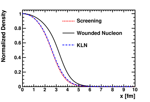
Therefore, in order to more naturally take into account the expected screening, we propose the following form for the energy density:

$$\epsilon(x,y)=K\frac{\sigma_{\text{inel}}}{\sigma}\frac{2T_{A}T_{B}}{T_{A}+T_{B}}\left[1-e^{-\sigma(T_{A}+T_{B})/2}\right]$$ (5.5)

where $\sigma$ is the cross-section associated with screening and should not be larger than the full inelastic cross-section. This form no longer has the property that it behaves like collisional scaling when one density is much larger than the other but instead reduces the energy density based on whichever nucleon density is smaller. This model achieves the same scaling in the limit that both nucleon densities are diffuse. In the higher density region the scaling described in Equation 5.5 behaves like participant scaling instead of collisional scaling and, in fact, in regions where the thicknesses are similar the model is the same as the wounded nucleon model. In regions where the thicknesses are very different, such as where the tails of one nucleus overlap with the center of the other nucleus in the transverse plane, the scaling described in Equation 5.5 falls off much faster than wounded nucleon scaling (Equation 5.3) as seen in Figure 5.1. This increases the eccentricity of the initial source which one naïvely expects should increase the produces elliptic flow with other parameters constant.

Up to this point, we have assumed that the nuclear thickness functions are smooth and interact probabilistically. One might also force the nucleons to interact locally and with precise locations through Monte Carlo methods. This is done by distributing nucleons in each nucleus by drawing from the distribution $4\pi r^{2}\rho(r)$ for radial positions of the nucleons and flat distributions for the azimuthal angle and the cosine of the polar angle. Draws are performed once for each nucleon in each nucleus involved in the collision. The nucleons are then assumed to be black discs in the transverse plane of radius given by the total proton-proton inelastic cross-section for the collision energy of interest. Collisions occur any time black discs overlap in the transverse plane with the longitudinal distribution ignored. One generally counts both the total number of pairwise collisions, the number of binary collisions ($N_{BC}$), and the number of nucleons participating in any collision, the number of wounded nucleons ($N_{WN}$). To generate an energy density profile, one can place Gaussians at the location of the participants or collisions with arbitrary normalization and width, though the width should certainly be no larger than the radius of the proton. This procedure produces lumpy and fluctuating profiles, but profiles without significantly different trends from the smooth variety of the wounded nucleon described in Equation 5.3 [58]. Furthermore, the design of the hydrodynamic model makes the study of fluctuations impossible.

Other improvements to the Glauber model have been considered at impressive length by the PHOBOS collaboration including variation of nuclear density profile parameters, the inelastic nucleon-nucleon cross-section, hardcore nucleon repulsion within the original nucleus, and several experimental considerations that would affect interpretation of the multiplicity results [58]. For reasonable variations of the parameters, they find only $\pm 5\%$ influence on results for collisions mid-central and central collisions for Au+Au collisions at $\sqrt{s}=200$ GeV where the largest deviations are for the experimental considerations. Also of note is that corrections for very peripheral collisions can be considerably larger, up to $\sim 20\%$. Furthermore, they investigate differences between using smooth density profiles and using the average of many Monte-Carlo events to determine multiplicity scaling. They find that for mid-central collisions, smooth profiles predict $\sim 10\%$ fewer particles produced by the 30-40% centrality bin for Au+Au collisions at $\sqrt{s}=130$ GeV.

One difficulty in comparing theoretical predictions to experimental data is that the impact parameter is not known for any particular event, though the smallest impact parameters should correspond to the highest multiplicity events. Geometrically it is clear that the change in probability of a particular impact parameter scales with the impact parameter, $d\sigma=2\pi b~{}db$, like circular shells for integration in polar coordinates. Integrating this equation and assuming that no collisions take place beyond a maximum impact parameter, the total cross-section is related to the maximum impact parameter by $b_{\text{max}}=\sqrt{\sigma_{T}/\pi}$. Experimentally events are separated into centrality classes which are the percentile of the total number of particles produced in a particular collision but reversed such that the 0-5% centrality class corresponds to the 5% of all events containing the most particles. As long as particle production falls monotonically with impact parameter, the relationship between the centrality class and the impact parameter should be

$$\frac{\%{\text{cent}}}{100}=\frac{\pi b^{2}}{\sigma_{T}}=\left(\frac{b}{b_{\text{max}}}\right)^{2}.$$ (5.6)

This allows one to calculate the average number of participant nucleon pairs for each centrality class, which one can compare to the total number of charged particles produced. Experimentally, the number of charged particles observed at midrapidity scales with the number of participants up to center of mass collision energies around $\sqrt{s}=100$ GeV [2]. At $\sqrt{s}=200$ GeV the deviation from this scaling is $\sim 5\%$ faster than linear, there are more observed charged particles than predicted by the number of wounded nucleons, from 0-40% centrality. Some groups have suggested that this implies an increasing importance of hard processes that might scale with the number of binary collisions and find that a mixture of 75% participant and 25% collisional scaling reproduces data at this energy [59].

A related theory that has had success predicting longitudinal rapidity distributions in d+Au systems is often called the Color-Glass-Condensate (CGC) [60, 61, 62, 8]. The assumption is that the gluon density distribution falls like the transverse momentum squared above a saturation scale ($Q_{s}^{2}$) but remain constant below it, an ansatz which proved very useful in describing the data collected in the HERA experiment [63]. The saturation scale depends on the density of partons in the original nuclei, generally taken to be the density of participants as defined in the Glauber model. There are many versions of CGC [8, 62, 64] that contain these features but there are not so many direct constraints on such inputs as the apparent gluon density distribution at some momentum scale. This leads to quite some number of unique models. We present the equations for generating CGC initial conditions in one particular model [8]. The scattered gluon density is given in terms of the original gluon distributions ($\phi_{A_{1}}$ for nucleus 1) as

$$\frac{d^{3}N}{d^{2}p_{T}dy}\propto\frac{1}{p^{2}_{T}}\displaystyle\int^{p}_{T}dk_{T}^{2}\alpha_{s}(k_{T})\phi_{A_{2}}(x_{1},k^{2}_{T})\phi_{A_{2}}(x_{2},(\vec{k}_{T}-\vec{p}_{T})^{2}),$$ (5.7)

where $x_{1,2}=(p_{T}/\sqrt{s})e^{\mp y}$ and y in the longitudinal rapidity. The unintegrated gluon distributions and saturation scale are given by

$$\phi_{A}(x,k_{T}^{2}) = \frac{1}{\alpha_{s}(Q_{s}^{2})}\frac{Q_{s}^{2}}{\max{(Q_{s}^{2},k_{T}^{2})}}\left(\frac{n_{\text{part}}^{A}}{T_{A}}\right)(1-x)^{4},$$ (5.8)

$$Q_{s}^{2}(x) = \frac{2T_{A}^{2}\text{GeV}^{2}}{n_{\text{part}}^{A}}\left(\frac{\text{fm}^{2}}{1.53}\right)\left(\frac{0.01}{x}\right)^{0.288},$$ (5.9)

where each is implicitly a function of the transverse position, rapidity, and nucleus. Also, $n_{\text{part}}^{A}$ is the participant density for nucleus A as given by the appropriate term of Equation 5.3. In this sense, the CGC is a reweighting of Glauber densities based on classical chromodynamics arguments about the saturation of gluon momentum distributions. Finally, we note that CGC models include rapidity dependence, which is one of its great successes notably for d+Au collisions [60] that is not predicted by Glauber models where that would be added ad hoc.

Figure 5.2: Comparison of the normalized transverse energy in initial conditions from KLN (green dashed), wounded nucleon (red dotted), binary collision (black solid), screening (blue dot-dash), and a mixture wounded nucleon and binary collision (gray double dot-dashed) chosen to reproduce experimental multiplicity scaling. Since the total overlap area scales with total particle production and normalization is set by the most central bin, all curves are defined to be unity at b=2.23 fm before dividing by the binary collision result at each impact parameter. The wounded nucleon model therefore predicts the slowest scaling of multiplicity with impact parameter while binary collision scaling would produce the most rapid scaling. The screening model and KLN predict similar scaling with impact parameter as the best fit mixture of wounded nucleon and binary collision scaling, therefore we expect these models to follow experimental data in this respect.

Figure 5.3: Schematic of source of initial eccentricity as it originates directly from the finite impact parameter [3]

Figure 5.4: Comparison of initial source eccentricity between KLN (green dashed), wounded nucleon (red dotted), binary collision (black solid), screening (blue dot-dash), and a mixture wounded nucleon and binary collision (gray double dot-dashed) chosen to reproduce experimental multiplicity scaling. Wounded nucleon scaling predicts the smallest initial source eccentricity and is not greatly increased by the inclusion of some binary collision scaling to reproduce multiplicity scaling. The screening model predicts the largest eccentricity of the models considered here, including KLN, though other CGC calculations of initial conditions predict eccentricities this large. This suggests theoretical uncertainty of roughly 50% in the source eccentricity that will propagate to uncertainty in the shear viscosity.

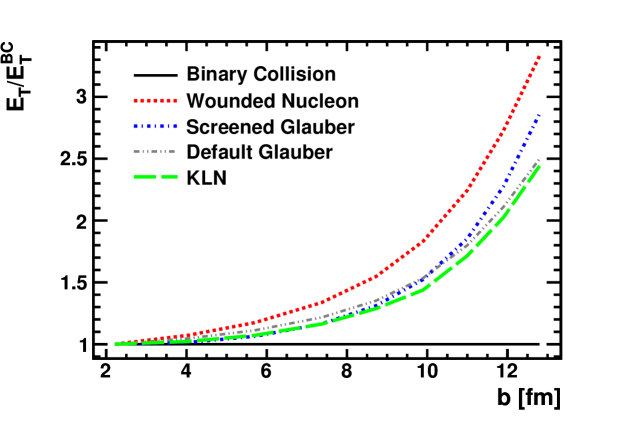
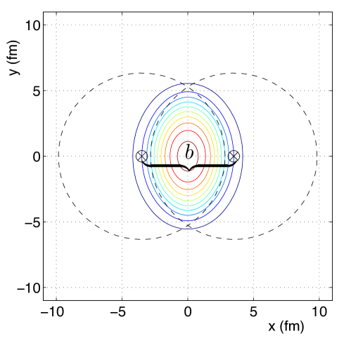
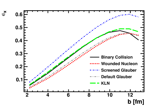
As stated before, there are many varieties of CGC and few of the parameters are well known so we consider only the energy density profile predictions. These profiles tend to predict higher initial source eccentricities and somewhat faster total density scaling with impact parameter than participant scaling in the Glauber model. To compare the scaling across models we compare the integrated energy density at midrapidity as a function of impact parameter. Each is normalized to give the same total number for the average central collision impact parameter with b=2.21 fm since this normalization is a free parameter in all of the models. For ease of interpretation, in Figure 5.2, we divide by the binary collision result. All the curves lie above one, meaning that collisional scaling predicts the most rapid scaling with impact parameter, while participant scaling varies the most slowly. The double-dot dashed (green) line shows the linear combination of collisional and participant scaling found to reproduce the data. Note that both the CGC variety and the simple saturation model given in Equation 5.5 predict similar scaling to this linear combination, and we therefore expect that these models will all predict similar multiplicity scaling with impact parameter.

Another important experimental observable affected by the initial condition is the elliptic flow. In the hydrodynamic picture, elliptic flow is the result of initial source eccentricity. Hydrodynamics generates flow in proportion to pressure gradients leading to faster collective expansion in the short direction of the source. Viewed in the transverse plane, the initial eccentricity comes from the overlap geometry of the overlapping nuclei. As shown in Figure 5.3, for impact parameters of roughly the nuclear radius, the overlap region is shorter along the impact parameter than in the orthogonal direction.

In addition to predicting different multiplicity scaling, models of initial conditions predict different initial eccentricities. Figure 5.4 shows the comparison of the eccentricity predicted by the various models for initial densities, as defined by

$$\epsilon_{x}=\frac{<y^{2}>-<x^{2}>}{<y^{2}>+<x^{2}>}$$ (5.10)

where the averages are over the transverse plane weighted by the energy density. Participant scaling turns out to produce the least source eccentricity for this set of models with the mixture of collisional and participant scaling that reproduces multiplicity scaling being almost as small. The screening model produces the most eccentricity of these models, but this is more a function of the choice of CGC model; others predict eccentricities as large or larger compared to the saturation model [8].

5.2 Initial Flow

5.2.1 Early Flow Model

The energy density alone is not enough to initialize even ideal hydrodynamics as the collective velocity is not determined. The early assumption of modelers was that the system should exhibit no collective behavior prior to thermalization and that the fluid should begin at rest in the transverse direction [65, 26, 66, 67] . This is in direct contrast to the longitudinal initialization, where boost invariance means that the system is borne with strong velocity gradients despite the lack of acceleration in any comoving frame. If the longitudinal treatment were translated to the transverse case, that would assume that particles free-streamed prior to thermalization, though this is not strictly a requirement for the longitudinal assumptions to hold.

Unfortunately, we find that the conclusions one would draw about the structure of the matter are sensitive to the assumptions one makes about the dynamics of the system prior to equilibration [68]. In fact, early hydrodynamic models using a very stiff equation of state predicted that the system would have to thermalize after only 0.1 fm/c to achieve the correct amount of flow in the total collision time suggested by the longitudinal extent of the system [22]. This result is not difficult to understand: the development of elliptic flow is initially parabolic for a system starting from rest so, as in a sprint, a difference in starting time is often more critical than top speed.

Model	$T^{xx}=T^{yy}$	$\tau^{2}T^{\eta\eta}$	$T^{\tau\tau}$
Longitudinal electric field	$T^{\tau\tau}$	$-T^{\tau\tau}$	$\sim$constant
Free streaming massless particles, two-dimensional relativistic gas or fields from incoherent longitudinal currents	$T^{\tau\tau}/2$	$0$	$\sim 1/t$
Ideal hydrodynamics of massless gas	$T^{\tau\tau}/3$	$T^{\tau\tau}/3$	$\sim 1/t^{4/3}$

Table 5.1: Elements of the stress energy tensor for simple models at early times [68]. A wide variety of reasonable values for the stiffness of the transverse equation of state are represented by the models.

This puts a premium on understanding the model dependence of the initial conditions to the hydrodynamic phase. We consider models in which the stress-energy is conserved, $\partial_{\mu}T^{\mu\nu}=0$, and $T^{0i}(\tau=0)=0$ for spatial indices due to symmetry. The models differ in terms of the their assumption about the relationship between $T^{00}$ and $T^{xx}$ and $T^{yy}$. As described in Table 5.1, this framework can describe a model based around longitudinal fields like the CGC, which would predict very strong transverse pressure and negative longitudinal pressure to ideal hydrodynamics, with complete transverse-longitudinal symmetry in terms of a single parameter $\kappa$ given by

$$\kappa=\frac{T^{xx}+T^{yy}}{2T^{\tau\tau}}=\frac{T^{rr}+r^{2}T^{\phi\phi}}{2T^{\tau\tau}},$$ (5.11)

where we include the equivalent polar form for use later. The value of $\kappa$ depends on the microscopic description of the matter, for instance $\kappa=1/3$ in ideal hydrodynamics while $\kappa=1$ for longitudinal classical fields. We assume that the stress-energy tensor is traceless which allows us to determine all of the elements of the shear tensor. We further assume that $\kappa$ varies with proper time but not with spatial coordinates, which implies that the important degrees of freedom do not depend on location though they may depend on time.

The evolution of the system is given by the conservation of the stress-energy tensor and the system of equations are closed by the value of $\kappa$. Since we are primarily interested in physics at midrapidity and in the early generation of flow, we will consider a one-dimensional system that varies only in the transverse direction undergoing a boost invariant expansion. For such a system, only the elements of the stress-energy tensor and $T^{\tau x}$ will be non-zero where $x$ is the direction of the density gradient.

For small velocities and neglecting the longitudinal expansion, the Euler equation is exact and

$$\frac{\partial v^{x}}{\partial t}=\frac{-\partial_{x}T^{xx}}{T^{tt}+T^{xx}}=\frac{-\kappa}{1+\kappa}\frac{\partial_{x}T^{tt}}{T^{tt}}.$$ (5.12)

Usually this implies that $T^{xx}$ behaves as the effective transverse pressure, and larger values of the effective pressure lead to more rapid expansion. The natural conclusion would be that models with larger values of $\kappa$ would lead to larger acceleration. The longitudinal expansion turns out to include a very important correction to this conclusion.

To see this, consider the equation of momentum conservation in polar-Bjorken coordinates

$$\partial_{\tau}T^{\tau r}=-\partial_{r}T^{rr}-\partial_{\phi}T^{\phi r}-\partial_{\eta}T^{r\eta}-\frac{T^{\tau r}}{\tau}-\frac{1}{r}\left(T^{rr}-r^{2}T^{\phi\phi}\right).$$ (5.13)

The final three terms are derived from affine connections but have simple explanations in Cartesian coordinates. The longitudinal expansion means that $v^{z}=z/t$ and therefore $T^{zx}\approx(z/t)T^{tx}$ for small $z$. Furthermore, if the system has rotational invariance, then

$$T^{xy}(y=0)\approx(y/x)(T_{xx}-T_{yy})=(y/x)(T^{rr}-r^{2}T^{\phi\phi}).$$ (5.14)

Initially and to first order in $u^{r}$ for the hydrodynamic case, $T^{rr}=r^{2}T^{\phi\phi}$. For the hydrodynamic case, both are roughly the pressure though there is a second order correction. More generally, the term is explicitly zero initially and we will assume that this term remains small.

Similar considerations for energy conservation yield the equations of motion

$$\partial_{\tau}T^{\tau\tau} = \frac{-1}{\tau}(T^{\tau\tau}+\tau^{2}T^{\eta\eta})-\left(\partial_{r}+\frac{1}{r}\right)T^{r\tau},$$ (5.15)

$$\partial_{\tau}T^{\tau r} \approx -\partial_{r}T^{rr}-\frac{T^{r\tau}}{\tau}.$$ (5.16)

where the approximation in Equation 5.16 is ignoring the term from rotational symmetry. The quantity that is of interest is the ratio $T^{\tau r}/T^{\tau\tau}$. In the hydrodynamic picture, this quantity scales linearly with collective velocity for small velocities and generally should be thought of like a normalized momentum density. We can easily calculate the proper time derivative to be

$$\partial_{\tau}\left(\frac{T^{\tau r}}{T^{\tau\tau}}\right) = \frac{\partial_{\tau}T^{\tau r}}{T^{\tau\tau}}-\frac{T^{\tau r}\partial_{\tau}T^{\tau\tau}}{(T^{\tau\tau})^{2}},$$ (5.17)

$$\partial_{\tau}\left(\frac{T^{\tau r}}{T^{\tau\tau}}\right) \approx \frac{-\partial_{r}T^{rr}}{T^{\tau\tau}}+\frac{\tau^{2}T^{\eta\eta}T^{\tau r}}{\tau(T^{\tau\tau})^{2}},$$ (5.18)

where we ignore second order terms, $(T^{\tau r}/T^{\tau\tau})^{2}$, including the term proportional to $\partial_{r}T^{r\tau}$.

For small times the change in this ratio is linear, so we can solve for the acceleration $\alpha(r)$,

$$\frac{T^{\tau r}}{T^{\tau\tau}} = \alpha(r)\tau,$$ (5.19)

$$\alpha(r) = \frac{-\partial_{r}T^{rr}}{T^{\tau\tau}-\tau^{2}T^{\eta\eta}},$$ (5.20)

where $\tau^{2}T^{\eta\eta}=T^{zz}$ is not small even for small proper times. We now employ all of our assumptions which are that

• the radial and azimuthal pressure remain the same – $T^{rr}=r^{2}T^{\phi\phi}=\kappa(\tau)T^{\tau\tau}$,

• the anisotropy of the stress-energy tensor is the same everywhere – $\kappa(r,\tau)=\kappa(r)$, and

• a traceless stress-energy tensor – $g_{\mu\nu}T^{\mu\nu}=0$.

This leads to

$$\alpha(r) = \frac{-\kappa\partial_{r}T^{\tau\tau}}{2(T^{rr}+r^{2}T^{\phi\phi})},$$ (5.21)

$$\alpha(r) = \frac{-\partial_{r}T^{\tau\tau}}{2T^{\tau\tau}}.$$ (5.22)

This means that the development of momentum density at small times,

$$\frac{T^{\tau r}}{T^{\tau\tau}}=\frac{-\partial_{r}T^{\tau\tau}}{2T^{\tau\tau}}\tau,$$ (5.23)

does not depend on $\kappa$. Therefore classical, longitudinal fields produce the same amount of flow as free streaming particles by this measure. This is exactly the opposite conclusion suggested by the Euler equation, Eq. 5.12, where we anticipated that the development of flow would be directly proportional to $\kappa$. Note that the boost invariant expansion is critical to this result. Furthermore, the result to first order is exactly twice the acceleration that one would predict from Eq. 5.12 which one might have anticipated from the tests performed in Chapter 4.

The choice to measure the pre-equilibrium flow as ratios of the temporal components of the stress-energy tensor was made with an eye toward thermalization. When the system undergoes a change in the underlying degrees of freedom, for example in the sudden decay of the longitudinal fields, conservation of the stress-energy tensor, $\partial_{\mu}T^{\mu\nu}=0$, should remain valid. As before, we assume that this transition is sudden in proper time, meaning that the transition hypersurface can be defined by a normal vector, $n^{\mu}=(1,0,0,0)$. Integrating the conservation equation across this hypersurface gives

$$0 = \int_{\tau-\delta\tau}^{\tau+\delta\tau}\left(\partial_{\tau}T^{\tau\alpha}+\partial_{i}T^{i\alpha}\right),$$ (5.24)

$$0 = T^{\alpha\tau}(\vec{r},\tau+\delta\tau)-T^{\alpha\tau}(\vec{r},\tau-\delta\tau),$$

where the term proportional to a spatial derivative is zero because $\delta\tau$ is small and that term is not divergent. This result means that, as long as the transition between descriptions is time-like, the temporal components of the stress-energy tensor cannot change suddenly. In the case that the system is suddenly thermalizing into an ideal hydrodynamic or Navier-Stokes viscous hydrodynamic system, these four components are sufficient to determine all the remaining components of the stress-energy tensor. The resulting flow profile could be rather different if one assumed thermalization to Navier-Stokes viscous pressures instead of the ideal pressures, though all of the early models would still produce similar flow profiles. Also, Israel-Stewart hydrodynamics does not prescribe the value of the six independent components of the shear tensor, $\pi^{\mu\nu}$, and therefore one would need a prescription to determine these values with possibilities including maintaining all the components of the stress-energy tensor.

If the transition is not time-like in the laboratory frame but is time-like in the comoving frame or even space-like, different elements of the stress-energy tensor might be conserved instead. This more general case can be summarized in terms of $n^{\mu}$, the surface normal fourvector, by

$$\delta(n_{\mu}T^{\mu\nu})=0,$$ (5.25)

and is often called the Rankine-Hugoniot relation when discussed in the context of hydrodynamic shock fronts. In the case of static surface facing the x-direction, the components $T^{x\mu}$ are conserved from which ideal hydrodynamics can be initiated as in the time-like case.

We are particularly interested in the influence of this flow precursor on the anisotropic momentum distribution observed in the final state, which is the second-Fourier component of the azimuthal momentum distribution

$$v_{2}\equiv\left\langle\cos{2(\phi-\phi_{\text{RP}})}\right\rangle,$$ (5.26)

where $\phi_{\text{RP}}$ is the azimuthal angle of the reaction plane, which should roughly lie along the impact parameter though fluctuations may mean that it deviates from this. This requires running a full hydrodynamic calculation to generate an emission isosurface, generating millions of particles as emitted from the surface, and following those particles through their many interactions before one can calculate the final effect. It is much more convenient is to use a hydrodynamic substitute that can be calculated directly from the stress-energy tensor. This measure has been proven useful as a proxy for the final observable [69, 65] and is often called the momentum-space anisotropy or eccentricity by analogy to Eq. 5.10. It is defined as

$$\epsilon_{p}\equiv\frac{\int dx_{T}(T^{xx}-T^{yy})}{\int dx_{T}(T^{xx}+T^{yy})}$$ (5.27)

which for free particles would be the same as $v_{2}$ up to a factor of roughly two [27]. Note that since the discontinuity to our system is time-like, $T^{xx}$ and $T^{yy}$ are not continuous and this measure of the expected $v_{2}$ can change dramatically during thermalization.

5.2.2 Three Scenarios

The previous subsection points out that one should expect the same development of flow from models with rather different underlying physics. We now consider those models in more detail to confirm that our findings hold for the range of hydrodynamic starting times considered possible. To do this, we calculate the predictions of each model and monitor the development of our flow measure and our anisotropic flow measure.

The models we consider are from the range $1/3\leq\kappa\leq 1$. The smallest value of $\kappa$ is for ideal hydrodynamics of a conformal fluid. Since the energy density is singular at $\tau=0$, it is convenient to transform to equations of motion for flow and scaled energy density,

$$w \equiv \frac{T^{\tau r}}{T^{\tau\tau}},$$ (5.28)

$$U \equiv T^{\tau\tau}\tau^{4/3},$$

where the choice of $\tau^{4/3}$ motivated by the expected rate of energy density decay for longitudinal ideal hydrodynamics. The equations of motion for $w$ and $U$ are derived from Equations 5.15 and 5.16 and are solved numerically for a fixed radial mesh.

The largest value of $\kappa$ is meant to mimic the effects of the CGC by considering a classical, coherent longitudinal electric field. This is not exactly what one expects from CGC models, as the fields should be coherent only on length scales corresponding to the saturation scale. On the other hand, this model provides an extreme example of how strong the effective transverse pressure could be with $T^{\tau\tau}\approx T^{rr}$ and the maximum value of $\kappa=1$. For a single pair of oppositely charged particles created at $x=y=0$, the Lienart-Wiechart form for the vector potential can be used to generate the electric and magnetic fields,

$$A_{z}(r,\tau) = 2q\int_{0}^{\infty}d\tau^{\prime}\delta(x^{2}+y^{2}-(\tau-\tau^{\prime})^{2}),$$ (5.29)

$$E_{z}(r,\tau) = 4q\delta(r^{2}-\tau^{2}),$$

$$B_{\phi}(r,\tau) = -E_{z}(r,\tau).$$

Then for the charge density $\rho(x,y)$, one can integrate over the charge density

$$E_{z}(x,y,\tau) = 2\int d\phi~{}\rho(x-\tau\cos\phi,y-\tau\sin\phi),$$ (5.30)

$$B_{x}(x,y,\tau) = 2\int d\phi~{}\rho(x-\tau\cos\phi,y-\tau\sin\phi)\sin\phi,$$

$$B_{y}(x,y,\tau) = -2\int d\phi~{}\rho(x-\tau\cos\phi,y-\tau\sin\phi)\cos\phi.$$

One can then calculate elements of the electromagnetic stress-energy tensor from

$$T^{\tau\tau} = \frac{1}{8\pi}\left[E^{2}+B^{2}\right],$$ (5.31)

$$T^{\tau i} = \frac{1}{4\pi}\left(\vec{E}\times\vec{B}\right)^{i},$$ (5.32)

$$T^{ij} = \frac{1}{4\pi}\left(E^{i}E^{j}+B^{i}B^{j}-\frac{\delta^{ij}}{2}\left[E^{2}+B^{2}\right]\right).$$ (5.33)

Since the region between the nuclei is charge-free, the evolution of the fields can be calculated by the conservation of the stress-energy tensor. The initial state of the charge density was chosen such that the resulting energy density profile would be the same as for other models. For the Gaussian profiles that we will consider in the next section, this means increasing the charge density radius by a factor of $\sqrt{2}$.

If instead the fields are generated by incoherent sources, that is arbitrarily oriented charged pairs receding from one another at the speed of light, Equation 5.29 still describes the fields due to each source. The arbitrary orientation means that the fields from each source will be arbitrarily oriented as well, but the elements of the stress-energy tensor are all the same because the energy density always moves outward from each pair. In this case the longitudinal electric field and the azimuthal magnetic field have the same strength which gives $T^{zz}=0$ and $\kappa=1/2$. This model thus behaves exactly the same as massless particles free-streaming in the transverse plane. This is not surprising as both models are of point sources emitting outgoing transverse waves, and the distinction between an electromagnetic pulse and partons is unimportant in the limit that the partons are massless.

These two electromagnetic models are meant in some sense as thought experiments but should bound a more realistic theory. The limit that the sources are point particles will break down at these length scales, which are roughly the length and time scales where the uncertainty principle is relevant. In low momentum QCD this coherence length is generally called the saturation scale and is approximated by $\lambda\sim 1/E$ where E is the typical energy of a parton. For time and length scales that are smaller than $\lambda$, the stress-energy tensor should be like the coherent limit of longitudinal classical fields, while at longer scales the incoherent limit should apply. This does not affect the result in Equation 5.23 as $\kappa$ is allowed to vary with time as long as it does not depend on location which is just what one would expect from these considerations.

5.2.3 Model Results

We initialize all three models – ideal hydrodynamics, incoherent field, and coherent fields – with Guassian profiles for the effective energy density

$$T^{\tau\tau}(x,y)\propto\exp\left\{-\frac{x^{2}}{2R_{x}^{2}}-\frac{y^{2}}{2R_{y}^{2}}\right\}.$$ (5.34)

Our focus will be the effect on the radial flow that would be present upon initializing an ideal hydrodynamics model with the equation of state of a massless gas – $P=\epsilon/3$. Recall that the time-like transition means that time-like elements of the stress-energy tensor are conserved – $T^{\tau\mu}$. This means that one can calculate the collective flow observed after the transition, denoted $u_{r}^{\prime}$, just from the ratio $T^{\tau r}/T^{\tau\tau}$:

$$T^{\tau\tau}=\frac{\epsilon}{3}\left(4\gamma^{\prime 2}-1\right),~{}~{}T^{\tau r}=\frac{4\epsilon}{3}\gamma^{\prime}u^{\prime}_{r}.$$ (5.35)

For the model that assumes ideal hydrodynamic evolution for the whole time, there is no change in the velocity and $u_{r}=u_{r}^{\prime}$. In other models this will not be the case. We investigate transitions at a few times that encompass the assumed range of starting times, $\tau=\{0.3,0.6,1.0\}$ fm/c, and we take the radii to be equal $R_{x}=R_{y}=3.0$ fm.

Figure 5.5: Bottom panel: The velocity of the frame in which $T^{0x}=0$ for coherent electromagnetic fields (blue squares), for incoherent fields or a non-interacting gas (red circles), and for an ideal liquid (green triangles) shown at three time steps, $\tau=\{0.3,0.6,1.0\}$ fm/c. The models predict significantly different amounts of radial flow, though in the opposite hierarchy suggested by the transverse pressure due to the effects of the Bjorken expansion. This quantity may change during thermalization.
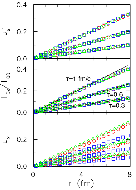
Middle Panel: The ratio of $T^{\tau r}/T^{\tau\tau}$ at the same times as the bottom panel, a measure of the flow developed in the early stage that will be maintained upon transition to ideal hydrodynamics. All the models predict the same evolution of this quantity up to 1 fm/c, which is roughly the domain of the model, and all are fairly well described by the linear approximation.
Top Panel: The collective velocity that would be apparent following transition to ideal hydrodynamics at the same three times as a function of radial position. Confirms that all of the models make the same prediction for the initialization of hydrodynamics.

For Gaussian profiles and to first order in time, Equation 5.23 gives the evolution of the flow

$$\frac{T^{\tau r}}{T^{\tau\tau}}\approx\frac{r\tau}{2R^{2}},$$ (5.36)

which using Equation 5.35 can be used to calculate the velocity before and after transition

$$u^{\prime}_{r}\approx\frac{3r\tau}{8R^{2}},$$ (5.37)

which are accurate to first order in time only but are useful to benchmark our expectations.

Figure 5.5 shows the results of all three models in terms of the velocity observed with the model itself (bottom panel), the conserved flow conserved by the transition to hydrodynamics (middle panel), and the flow observed within the hydrodynamic model following the transition (top panel). The results for the velocity observed within each model show considerably different results depending on the effective transverse pressure of that model. Somewhat counterintuitively, the ideal hydrodynamic model predicts the largest amount of apparent pre-equilibrium collective velocity despite having the smallest pressure, $\kappa=1/3$, while the coherent field model, $\kappa=1$, predicts the largest value. However, even for times up to $\tau\approx 1.0$ fm/c, the ratio $T^{\tau r}/T^{\tau\tau}$ is quite well approximated by the linear estimate in Equation 5.37, shown as a solid line, and all the models track with one another even more closely. Finally, we include a demonstration that this produces the same flow within the hydrodynamic model though this is guaranteed by the temporal elements of the stress-energy tensor being the same.

Figure 5.6: (Color in electronic version) Bottom Panel shows the momentum space anisotropy apparent within each model. Free-streaming particles (red circles) produce no apparent anisotropic flow while coherent fields (blue squares) produce much less than the analytic result of Eq. 5.39 which is accurate to first order in time for ideal hydrodynamics (black line).
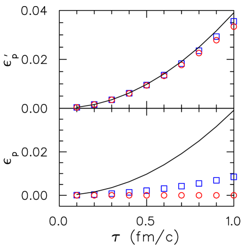
Top Panel shows the momentum space anisotropy observed in an ideal hydrodynamic model if the early flow model thermalized suddenly at that time. All of the models produce the same elliptic flow in the hydrodynamic source at very early times though they differ slightly by $\tau=1.0$ fm/c. This helps to explain why the matter created at RHIC appears to thermalize instantly.

While the development of radial flow is somewhat important in determining the average transverse momentum and can have some effect on the collision time, the elliptic flow is of greater concern. This is for two reasons, early times affect elliptic flow more dramatically and the discriminating power of elliptic flow is expected to be larger for interesting theoretical parameters like the shear viscosity. Since anisotropic flow is the result of eccentricity of the initial density, we alter the initial profile by change the radius in the y-direction to be $R_{y}=2$ fm instead of 3 fm. We then run the same calculation as above for the coherent and incoherent fields in the transverse plane. Development of anisotropic flow is calculated in terms of the difference of stress-energy tensor elements as defined by $\epsilon_{p}$ in Equation 5.27. Figure 5.6 shows the apparent anisotropic flow within the model itself (bottom panel) and contrasts that with the anisotropic flow that would be apparent in the hydrodynamic model if it were initialized at that time. Models based on free-streaming particles or incoherent fields (red circles) do not generate any anisotropic flow at all, while coherent fields generate considerably less than an estimate of the flow generated by ideal hydrodynamics. And yet, whenever the system undergoes thermalization, the conservation of the time-like components of the stress-energy tensor mean that flow immediately appears regardless of the previous description.

For short times, the flow generated in either direction was given by Equation 5.37 to be

$$u_{x}\approx\frac{3}{8}\frac{x\tau}{R_{x}^{2}},~{}~{}~{}u_{y}\approx\frac{3}{8}\frac{y\tau}{R_{y}^{2}}.$$ (5.38)

One can then calculate the momentum anisotropy directly using a few Gaussian integrals to be

$$\epsilon_{p}\approx\frac{9\tau^{2}}{32}\left(\frac{1}{R_{x}^{2}}-\frac{1}{R_{y}^{2}}\right)$$ (5.39)

which is plotted as a solid line in Figure 5.6. For short times, this approximation describes all of the models well, though it begins to overestimate the effect by 1.0 fm/c due to the asymmetric expansion of the source reducing the eccentricity of the transverse energy density.

The effects of this on final elliptic flow will be discussed at greater length below, but we emphasize that the argument’s main thrust is that a reasonably large class of models all produce the same predicted input for ideal hydrodynamics in terms of collective flow. Non-zero flow at the onset of hydrodynamics explains why early hydrodynamics models overestimated the longitudinal size of the source, when they used a reasonable time, $\sim 1.0$ fm/c, for the onset of hydrodynamic behavior. Including this pre-equilibrium flow causes the system to dissipate more quickly and decreases the longitudinal size. Also of note is that our conclusion is independent of whether or not the model for early times appears to contribute to anisotropic flow, instead it only depends on the transition to ideal hydrodynamics. We expect that this conclusion would remain true for a transition to Navier-Stokes hydrodynamics since the same ratio, $T^{0x}/T^{00}$ is sufficient to determine the collective velocity in that case as well.

5.3 Initial Shear Corrections

The remaining six variables to be determined for initializing a viscous hydrodynamics code are components of the shear tensor. In Israel-Stewart hydrodynamics, each of these moments is an independent variable that cannot be determined from other hydrodynamic information such as the energy density and velocity gradients. If there were an underlying gas description prior to the time of thermalization, one could calculate the full stress-energy tensor from moments of the momentum distribution. Lacking that, if the system were very near to equilibrium, one might assume that the Navier-Stokes equation would give a good approximation to the shear elements. This turns out to be difficult for reasons discussed above – namely, the corrections do not get small as rapidly as the pressure. The shear viscosity is proportional to the entropy density and thus diverge slowly, like $\epsilon^{-1/4}$. This means that for any initial condition with a longitudinal velocity gradient there will be some small temperature below which corrections to the pressure are larger than the pressure.

This can happen even for moderately small viscosities ($\eta/s\approx 0.16$) at relevant temperatures ($T\approx 100$ MeV), where the value of $|\pi^{zz}|$ approaches not just the pressure but the energy density. If $\epsilon+P+\pi^{zz}=0$, the conservation of longitudinal momentum equation is singular and the resulting correction to the longitudinal velocity diverges. For Navier-Stokes conditions this is true when

$$0=(\epsilon+P)\left[1-\frac{4\eta}{3T_{b}s\tau}\right],~{}~{}T_{b}=\frac{4\eta}{3\tau s},$$ (5.40)

where $T_{b}$ is the temperature at which the hydrodynamic equations of motion can no longer be solved. Since $\eta/s$ is often taken to be a constant, any choice of $T$ and $\tau$ will eventually have this divergence issue. The problem is even worse if the shear viscosity to entropy density ratio rises rapidly in the gas phase as one would expect when moving away from a phase transition.

Extreme viscous corrections are not always a dynamic problem in the Israel-Stewart framework: if the system does not begin with excessively large corrections they will not develop. The relaxation time is proportional to shear viscosity, meaning that in regions where large corrections would be expected in the Navier-Stokes theory, the Israel-Stewart theory allows the system to approach such large corrections only slowly. Of course, this also means that if large corrections exist in the system at the onset of hydrodynamics they will remain large and if the density falls faster in the tails due to the longitudinal expansion than it rises due to transverse flow the problem will worsen. Regardless of these details, while the picture that Israel-Stewart theory is a relaxation toward the Navier-Stokes theory is somewhat naïve, it does tend to prevent aberrant behavior outside of the freezeout surface for not unphysical initial conditions.

Previous studies considering the potentially large corrections in the tails have taken a variety of tacks. A popular choice is to initialize the shear tensor to zero. This reduces the overall effect of shear viscosity on the fluid and thus in comparing produced anisotropic flow to data one finds an upper bound on the shear viscosity at the expense of the attempting to determine the actual value. Another choice is to treat the problem as one of regularization and therefore treat the region outside of the freezeout surface differently, for instance the comparison code used in Chapter 4 applies a position dependent suppression of the shear viscosity. Such an approach defies the natural structure of the code and might need to be adjusted for each parameter set which would become especially problematic when exploring systems at different impact parameters.

Another approach that would give proper reduction of the corrections in the tails would be to allow the shear viscosity to scale with the energy density below some temperature. This choice reduces corrections in the tails and prevents dynamical issues that occasionally arise for cases with large shear viscosity. For the boost invariant case, allowing the shear viscosity to scale with the energy density instead of the entropy density did not affect model predictions as long as this rescaling temperature was more than 20 MeV less than the freezeout temperature. This was expected since the output from the hydrodynamic module is the freezeout surface itself and not the entire evolution, and one expects the motion of matter from inside to outside to be more important than the reverse.

In addition to allowing the shear viscosity to decrease at low temperatures, we also scale the initial shear tensor to the pressure everywhere. This measure helps to keep corrections sane everywhere but also allows for the possibility that the system is too far from equilibrium at the beginning of the calculation for Navier-Stokes to be a good description. For instance, if the system were described by the coherent fields described above and the longitudinal direction were roughly pressure-free at the beginning of the evolution, this could be modeled. The coefficient scaling the initial corrections to the pressure is introduced as an input parameter to the model and its influence will be investigated in the next chapter.

Chapter 6 Results and Conclusions

6.1 Longitudinal Flow Results

The unique feature of the code discussed here is the inclusion of both viscosity and non-trivial longitudinal expansion. Generally, viscous hydrodynamic codes were written assuming a boost invariant expansion making the non-trivial evolution take place in only two dimensions though the system does expand longitudinally. We begin by investigating the approximation that the features of the expansion away from mid-rapidity are not important. To do this we choose a typical set of initial conditions and compare the evolution of hydrodynamic quantities at midrapidity with the full expansion to the same conditions under the assumption of boost invariance.

We begin the hydrodynamic evolution at $\tau_{0}=0.8$ fm/c. The initial transverse energy density distribution is taken from the Glauber model with a mixture of 85% wounded nucleon scaling and 15% binary collision scaling as described in Chapter 5 with the initial energy density for the central collision, b = 2.21 fm, as $\epsilon(0)\approx 19.5$ GeV/fm³, to reproduce pion multiplicities and scaling respectively for $\sqrt{s_{\text{NN}}}=200$ GeV Au+Au collisions. In the longitudinal dimension, we choose a Gaussian with scale $\sigma_{\eta}=1.4$ units in spatial rapidity; that is, $\epsilon(\vec{r})=\epsilon(x,y)\cdot\exp(-\eta_{s}^{2}/2\sigma_{\eta})$. While this is in contrast to other models that choose a long flat region of several units of rapidity with steep half-Gaussian tails [67, 66], a Gaussian profile is motivated by the experimental data which shows little deviation from this profile over a wide range of beam energies [5]. An improvement to the model would account for the angular momentum of the hot region momentum due to the non-zero impact parameter and for the breaking of longitudinal symmetry away from the symmetry axis between the nuclei. These improvements would be required to model directed flow away from midrapidity for any finite impact parameter, but for simplicity both were ignored in these tests. The initial flow was taken from the universal flow model discussed in the previous chapter, but only as half of the result predicted by Equation 5.23. In the longitudinal direciton, we assume that the matter is not moving collectively relative to the boost invariant expansion. And finally, we take the initial longitudinal pressure correction to be half the pressure, $\tilde{\pi}^{zz}=P/2$, and the transverse components to be equal to each other and to half the longitudinal value so that the shear tensor remains traceless. All off-diagonal elements are taken to be zero in the frame of the matter. The shear viscosity is taken to be $\eta/s=0.16$ for the hydrodynamic portion and to scale with the energy density below temperatures of 100 MeV. Finally, a recent lattice equation of state [6] was used for the hot region and the equation of state was forced to match an equilibrated hadron resonance gas below T=150 MeV via the procedure discussed in Chapter 3.

The integration region was made up of fixed cells in configuration space with grid densities of $dx=dy=d\eta_{s}=0.15$[fm], and a maximum proper time step of $d\tau=0.05$ fm/c using the methods described in Section 4.1.5. Since the system is reflection symmetric in every spatial dimension, only one octant was integrated with boundary conditions that enforce symmetries across the boundaries. Cells with temperatures below 30 MeV were culled and the hydrodynamic module was run until all cells in the integration region passed below T=150 MeV. For comparison, the same conditions were also run with boost invariant conditions.

Figure 6.1: Comparison of the energy density along the x- and y-axes at midrapidity at $\tau=5.52$ fm/c from a boost invariant and full 3d hydrodynamic treatment. While the central energy density falls more rapidly when the longitudinal expansion is included due to the increase in the longitudinal velocity gradient, which can be seen by observing that both 3d lines (red full and black dotted) are systematically lower than their 2d counterparts (blue dot-dashed and green dashed). The difference diminishes in the tails of the distribution but is roughly 5-10% at the center of the fireball.

Figure 6.2: The longitudinal velocity gradient multiplied by the proper time with the trivial boost invariant portion ($1/\tau$) removed so that boost invariant solutions would be exactly zero. The increase in the expansion rate is taken at the center of the fireball for impact parameters corresponding to centralities 0-5%, 10-20%, and 20-30% respectively. The behavior of the increase gradient in the velocity gradient appears to be independent of impact parameter at early times and follows a fairly characteristic behavior as the system matures. This explains the faster decrease in the energy density observed in Figure 6.1.

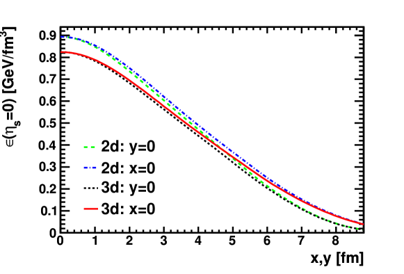
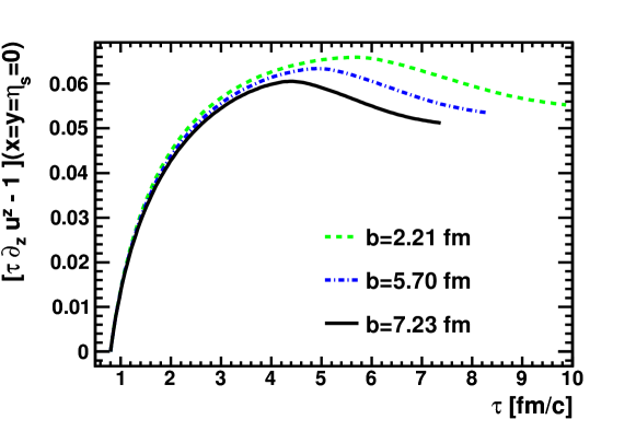
The simplest way to look for changes due to the nontrivial longitudinal expansion is to look at the values of the hydrodynamic fields along the symmetry axes of the system. Figure 6.1 shows the energy density along the transverse axes at midrapidity at a time after the system has gone through a bit over half of its evolution. We find that the energy density falls more rapidly in the center of the system in the 3d case, while the tails in the transverse direction are relatively unaffected. At the center of the fireball where the effect is the largest, the difference is less than 10%. We expect the difference to continue to grow as the expansion progresses, and therefore the source lifetime might be decreased by up to 20% which we will investigate below.

This more rapid decrease of energy density comes from a more rapid expansion in the longitudinal direction when the non-trivial expansion is included due to the density gradient in spatial rapidity. The increased expansion is demonstrated well by Figure 6.2 which shows the longitudinal velocity gradient at the center of the fireball with the effects of the boost invariant expansion removed. For a boost invariant expansion, this would be $\partial_{z}u^{z}=1/\tau$. Therefore, in the boost invariant scenario, this measure would be exactly zero. For the scenario with non-trivial longitudinal expansion, this measure is positive because the expansion accelerates due to the presence of longitudinal density gradients. The Gaussian shape produces linearly increasing longitudinal velocity as a function of proper time for small proper times near midrapidity that depends only on the longitudinal Gaussian radius. This is demonstrated by the centrality independence of the longitudinal expansion rate at early times. The longitudinal expansion is then slowed by viscosity, which tries to equalize the much more rapid longitudinal expansion with the burgeoning transverse expansion, and by the flattening of the density distribution due to the non-trivial longitudinal expansion itself. The increasing of the expansion rate lasts longer for central collisions but saturates in the same manner around a $5\%$ increase in the expansion rate compared to the boost invariant case for the latter half of the evolution. Since the longitudinal expansion rate is increased by about the same amount as the energy density at the center of the fireball is decreased compared to the boost invariant result, it would seem that the more rapid decrease in energy density can be attributed entirely to the non-trivial expansion and a more complicated explanation need not be sought.

Figure 6.3: The transverse velocity along the x- and y-axes at midrapidity for hydrodynamic simulations with and without boost invariance at $\tau=5.52$ fm/c. The transverse collective velocity is altered by less than 1% at midrapidity by the presence of a non-trivial boost invariant expansion. This suggests that elliptic flow observables at midrapidity do not require a full treatment of the longitudinal direction unless other factors on the basis of the hydrodynamic evolution itself.

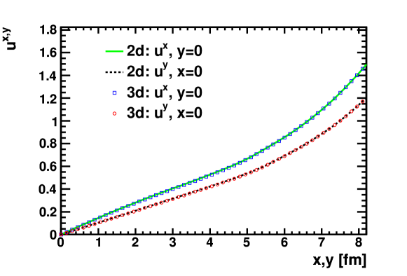
If the energy density is affected in the center of the fireball at the 10% level, one might be concerned that the transverse collective velocity might be affected in the same way. Such a result would be important for flow observables and might propagate to the parameter extraction based on these results. Figure 6.3 shows that this is not the case as the transverse collective velocity at the same time is affected by less than 1%. Apparently the transverse collective velocity is unaffected by the flatter distribution in the core, and any other effects from the longitudinal expansion are unimportant to the description of the system at midrapidity. This suggests that (2+1)d hydrodynamic results are trustworthy for midrapidity flow results, unless secondary influences like source lifetime or twisting provide unexpected corrections.

Figure 6.4: The position of the freezeout surface along the x-axis as a function of the proper time for collisions at three centralities. In each case the full integration shows the surface falling apart sooner but with very similar structure to the boost invariant case. This indicates that boost invariant treatments might overestimate longitudinal source lengths by 5% but dramatic change to the results is unlikely.

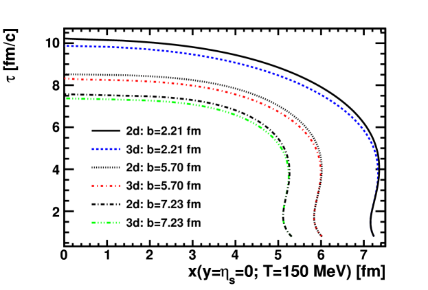
Finally, we investigate the motion of the freezeout surface at midrapidity. In the hybrid model that we will investigate later in this chapter, the location of the freezeout surface and the values of hydrodynamical fields there are the output of the hydrodynamical module to the hadronic cascade. Figure 6.4 shows exactly what one would have anticipated from Figure 6.1 – the general structure of the freezeout surface is not drastically altered. Rather the system dissipates sooner but without significantly altering the character of the motion. Given that the collective velocity and the motion of the surface are not significantly altered, it is difficult to imagine that theoretical conclusions regarding observables like the the anisotropic flow of the system will be significantly affected at midrapidity by including the longitudinal dynamics more completely.

However, we do expect the longitudinal source sizes to decrease if the system cools more rapidly at the 5-10% level. This is due to the relationship of the longitudinal source size to the duration of the collision and the Bjorken expansion. The Bjorken expansion means that in the center of momentum frame, the longitudinal collective velocity grows proportional to time. Since HBT is sensitive to the ratio of the collective velocity to the thermal velocity, there is a direct relationship between the duration of the collision and the longitudinal source size measured by HBT. Therefore more rapid decay of the thermal source will result in a smaller longitudinal radius. The overestimation of the longitudinal source size was a major issue in early hydrodynamic modeling [70], though pre-equilibrium flow also plays a role in the resolution of the so-called HBT puzzle [23].

There remains the possibility of more complicated model response to parameter changes but there is no evidence of this in these hydrodynamic results. One possible avenue for investigation would be to use midrapidity freezeout surfaces even from the full calculation and compare to boost invariant hydrodynamic calculations. Since there is little evidence that there would be any effect from this, we instead abstain from drawing further conclusions until we have a more complete treatment of the dynamics away from midrapidity including the non-zero chemical potential and angular momentum of the hot region. Both of these effects are good candidates for future work with this code.

6.2 Boost Invariant Results

We turn our attention to the boost invariant case and investigate the predictions of the whole model where we can make direct comparisons to the experimental data. This entails producing many particles and looking at quantities averaged over a large number of collisions. While experiment observes particles at a very wide range of momenta, our goal is only to study the behavior of the many lower mass particles produced at low momentum that come from the thermal source and to ignore the effects of hard processes that produce the remaining high momentum and large mass particles. Our interest is in determining constraints on the structure of the quark matter described by the hydrodynamic phase. For instance, it would be of great interest to determine the shear viscosity of the quark matter and whether the equation of state calculated by the lattice is supported or constrained by the experimental data. In addition, improvements to the hydrodynamics module that would allow the inclusion of known effects, such as the twisting of the source, have the potential to spoil the agreement with experimental data.

The experimental data that we will consider here are the distribution of low momentum, low mass particles produced in central and mid-central collisions of gold nuclei at center of mass energy $\sqrt{s_{\text{NN}}}=200$ GeV. We consider data only at midrapidity where effects of non-zero baryon number are expected to be small and the boost invariant code can make predictions. Specifically, we look at the spectrum of charged pions, kaons, and protons produced in the 0-5%, 10-20%, and 20-30% most central collisions which correspond to average impact parameters of 2.21, 5.70 and 7.37 fm respectively [9]. Looking at multiple centralities allows one to test the scaling of total particle multiplicity predicted by the various initial condition models. Anisotropic flow in the most central collisions is dominated by fluctuations that are not present in the initial conditions that we produce. Therefore, only multiplicity data is used the most central bin: the pion multiplicity sets the energy scale, while kaon and proton might be useful for constraining other parameters. Incorrect eccentricity in the most central bin might be overcome by reorienting the reaction plane in a Monte Carlo simulation to produce a realistic estimate of the initial eccentricity for a central event. This results in more turbulent initial conditions with steeper tails that can cause instability in the simulation.

6.2.1 Initial State Uncertainty

As mentioned in the previous chapter, there is significant uncertainty in the structure of the initial state of the hydrodynamic phase. This uncertainty is not limited to the shape of the hot region but also the collective velocity and the six independent elements of the shear tensor. While other groups have investigated effects of varying the shape of the source and the shear tensor within reasonable theoretical bounds, we further include the effect of including initial flow on spectrum and flow observables.

We first consider a set of model runs that were run at some interesting corners of the theoretically allowed parameter space. For this, the full model was run with 27 different parameter settings coming from all possible combinations of three settings for the three initial energy density models, three settings for the initial flow, and three settings for the initial longitudinal pressure. The models for the energy density are a Glauber mixture with 85% participant scaling which we will refer to as the default Glauber model, the saturation model described in Equation 5.5, and a smooth CGC model provided by Drescher et al. [8] referred to in Chapter 6 as KLN which predicts the entropy density instead of energy density and must be converted through the equation of state. The initial flow settings were the traditional setting of zero initial flow, half of the initial flow predicted by Equation 5.23, and the full prediction of the same. The initial value of the shear tensor is taken to be the set $\tilde{\pi}^{zz}=-\tilde{\pi}^{xx}/2=-\tilde{\pi}^{yy}/2=\{0,P/2,P\}$ respectively.

Figure 6.5: Pion spectra at midrapidity for the most central (0-5%) bin of Au+Au collisions at $\sqrt{s}=200$ GeV as a function of transverse momentum. The (black) line with squares is minimum bias data from the PHENIX experiment [9] corrected for experimental acceptances and efficiencies. The colored symbols are for three model runs with different initial conditions for the energy density where all three models have been tuned to reproduce the total number of pions between $p_{T}=$ 200 MeV and 1 GeV. All of the models are easily capable of reproducing the total multiplicity and there is not much variation in the slope meaning that this observable is not likely to have significant resolving power.

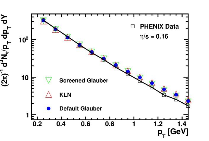
The normalization for the total size and energy of the hot region is a free parameter in all of the initial condition models that we consider. For this study we wished to separate effects due to the normalization from those due to the varied parameters. This requires running the hydrodynamic evolution with a guess for the normalization, running the cascade module from particle generation until collisions cease, and then tallying particles within the various transverse momentum bins in consideration. This process was automated by a short Python script that was used to determine the normalization for each set of initial conditions by comparing the number of low momentum pions produced to that measured by the PHENIX experiment between $p_{T}=$ 200 MeV and 1 GeV [9]. Figure 6.5 shows the low momentum pion spectrum compared to model runs with each flavor of initial energy shape. There is almost no variation between the model runs once they have been tuned to reproduce the normalization, and all of the parameter settings produce spectra that are too flat or overestimate the average transverse momentum. Some of this discrepancy can be attributed to the choice of maximum initial flow, but generally we have found that models that reproduce the normalization somewhat overestimate the average transverse momentum. This appearance of the effect is exaggerated in the figure by the inclusion of higher momentum particles. Bose corrections in the cascade or increasing the freezeout temperature may help soften the spectra, but the overestimation of the transverse momentum is 5-10% in these runs. This is roughly the same as the level of variation between the experiments [2].

Figure 6.6: Number of pions as a fraction of the number measured in the PHENIX experiment in the low momentum window $p_{T}=$ 200 MeV and 1 GeV displayed as a function of the impact parameters corresponding to the 0-5%, 10-20%, and 20-30% centrality bins. The Glauber model with 85% participant scaling most accurately describes the experimental scaling with all runs within 6% of the correct multiplicity though a clear trend to under predict the multiplicity at larger impact parameters. Both the Glauber saturation and the fKLN models under-predict the number of pions by roughly 10% in both of the mid-central bins. Allowing the scattered gluon density to be proportional to the entropy density instead of the energy density would help to counteract this issue.

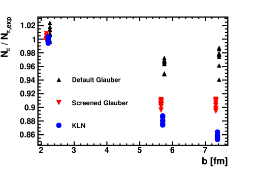
If we investigate the same quantity for larger impact parameters, we unfortunately find that none scale correctly. Figure 6.6 shows the pion multiplicity divided by the experimental pion multiplicity as a function of impact parameter. The default Glauber model most closely tracks with the data, though it is worth noting that the fraction of participant and collisional scaling is tuned to reproduce this data. However, the other two models under-predict the experimental scaling by 10-15% in both the 10-20% and the 20-30% centrality bins which is concerning. This is an unexpected result based on a naive interpretation of Figure 5.2, which showed that the integrated density of the Glauber mixture and the saturating Glauber have roughly the same scaling with impact parameter. In principle, the deviation of the screening model and the KLN model might be addressed by allowing the scattering densities to scale with the entropy density but it is our opinion that energy scaling is more justified. Notice also that the initial condition model has by far the largest effect on the multiplicity scaling as one would expect, although for the default Glauber model the variation within model runs due to initial flow and anisotropy can be as large as 5%. We note that it is possible that the multiplicity scaling errors observed in Figure 6.6 may affect the flow results, for instance by reducing the lifetime of the hot region, but our assumption is that it will not affect the model response to other parameter changes. Furthermore, later explorations of the larger parameter space will help illuminate this possibility.

Figure 6.7: Anisotropic flow for pions as measured by the PHENIX collaboration (black squares and line) for events in the 20-30% centrality bin as compared to model calculations with differing models for the initial energy eccentricity. For this choice of the shear viscosity, both of the saturation models significantly overpredict the experimental data while the default Glauber model describes the data.

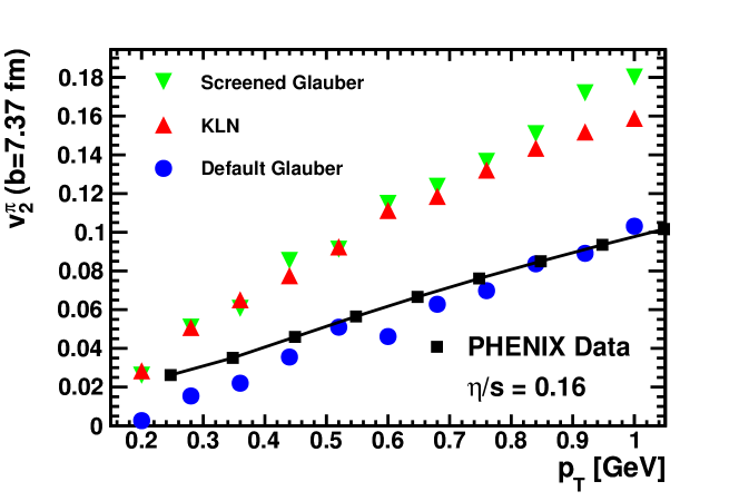
We now turn to our main focus which is on the influence of modeling choices in the initial state on the measured anisotropic flow ($v_{2}$), specifically whether the initial velocity or the initial shear pressure in the system strongly affect conclusions about the value of the shear viscosity near the critical temperature. As noted above, flow anisotropy in central collisions is expected to be dominated by fluctuations not present in our initial conditions and therefore we expect to under-predict the data in central collisions. Figure 6.7 shows the anisotropic flow as a function of transverse momentum for the same set of model runs shown in Figure 6.5 with a shear viscosity near to what other groups have found, $\eta/s=0.16$. Statistical fluctuations are still present in the model output but the integrated $v_{2}$ was found to fluctuate by less than one percent of the signal for a set of test runs in which the statistics were doubled. The default Glauber comes the closest to describing the data, again a conclusion that we have in common with some studies [71] though not all [27], but our model does show a different scaling with transverse momentum than the data. This has been observed in other simulations with significant shear viscosity and seems to come from the viscous corrections to the phase space density at freezeout [72, 73]. There is some ambiguity in this area, discussed in the previous chapter, and one would generally expect the phase space distortion due to the viscous corrections to the stress-energy tensor to be smaller for pions than for protons since the relaxation time for pions should be shorter once the species move independent of one another. This is not included in the freezeout algorithm presently but may explain this deviation. Also, the saturation models that predict larger source eccentricities also produce much larger elliptic flow, and in this case they over-predict the data by a factor of two.

Figure 6.8: Anisotropic flow for pions as measured by the PHENIX collaboration (black squares and line) for events in the 20-30% centrality bin as compared to model calculations with differing models for the initial energy eccentricity. Compared to Figure 6.7 the shear viscosity assumed in the fluid stage of the model is doubled. This leads to the saturation models giving a more accurate prediction while the default Glauber model now significantly under predicts the data. This suggests that the shear viscosity will be difficult to determine independently from the initial energy eccentricity without additional experimental data.

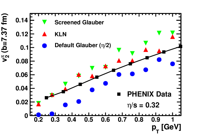
The same calculations were run with the shear viscosity doubled and the analogous plot is Figure 6.8. The default Glauber model now significantly under-predicts the experimental data especially at lower momentum, while the saturation models are in much closer agreement with the data. Also note that the range in which the elliptic flow is consistent with zero now extends up to 300 MeV for the default Glauber initial conditions, and also that the saturation models appear to develop this same feature at low momentum. Together with Figure 6.7, we find that uncertainty in the initial energy density profile contributes at least a factor of two in the uncertainty of the shear viscosity based solely on pion elliptic flow observables. This means that shear viscosity of at least 4-5 times the proposed conformal limit [74] may be consistent with this data.

Figure 6.9: The transverse momentum weighted, integrated anisotropic flow for the 20-30% centrality bin from the set of model runs described in the text. The runs are separated first by the source eccentricity due to the model choice for the initial state along the x-axis, where the default Glauber model predicts the smallest initial eccentricity followed by the KLN model and the screened Glauber model. The model runs are then colored by the initial anisotropy of the shear tensor with the largest initial anisotropy as downward-pointing (red) triangles, no initial anisotropy as upward-pointing (black) trianges, and halfway in between as (blue) circles. If initial anisotropy were an important factor in determining the elliptic flow, the symbols of one color would be systematically above or below the others. However, ordering appears random and not at all systematic and therefore the initial value of the shear tensor appears to have no effect on the final anisotropic flow. Also of interest is that the initial eccentricity and elliptic flow do not scale with each other when moving between initial energy density models: the CGC model and Glauber screening model have initial eccentricities that differ by 20% but predict the same elliptic flow to within a few percent.

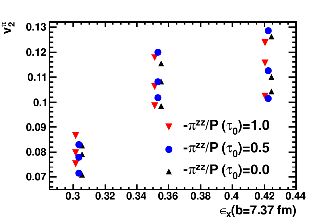
As noted above, the energy density is only one of the ten hydrodynamic variables that need to be set in the initial condition. Six of the other variables are the viscous corrections to the stress energy tensor. Boost invariance and the absence of bulk viscosity constrain four of these variables, and the further assumption that in the frame of the matter the transverse coordinates should be equivalent means that there is only one shear correction to be set. It is convenient to set the longitudinal pressure correction. This is allowed to vary from zero to the pressure, $0<\pi^{zz}<P$, where zero would coincide with complete local equilibration and $P$ would coincide with a description in terms of free streaming particles. This should cover the majority of the parameter space for this initialization for a fixed thermalization time, as corrections larger than the pressure are unlikely to be well modeled by even the second-order viscous equations of motion used. Figure 6.9 shows all of the model runs performed with the smaller viscosity value colored in the figure according to the initial longitudinal pressure correction. The variance within the model output appears to have no connection to the initial anisotropy, for instance, the output for runs with no initial longitudinal pressure are not systematically above or below the other runs. The symbols are frequently found in sets of three and in random order even within those sets, meaning that the initial shear tensor has no systematic influence on model output.

That the initial value of the anisotropy is not an important parameter for elliptic flow is not unexpected. Regardless of the initial condition, the shear tensor will relax toward the Navier-Stokes values on a time scale set by the relaxation time. This means that the initial value no longer plays a role for time scales longer than the relaxation time. For temperatures relevant to the hydrodynamic phase, the relaxation time is less than 1.0 fm/c, for the shear viscosity to entropy density ratio used in these simulations, meaning that the initial value only influences a small fraction of the evolution.

Figure 6.10: The transverse momentum weighted integrated anisotropic flow for the 10-20% centrality bin from the set of model runs described in the text displayed in the same manner as Figure 6.9. The model results are colored by the initial velocity as a fraction of the results from Equation 5.23 ($\chi_{f}$) where the (red) downward triangles are the full result, the (blue) circles half, and the (black) upward facing triangles with no initial velocity. The variation of results within each initial density model is shown to be explained by the changing of the initial flow as all of the runs are well-ordered by the strength of the initial flow. The initial anisotropy, which are not differentiated from one another, produce small, random changes in the observed elliptic flow.

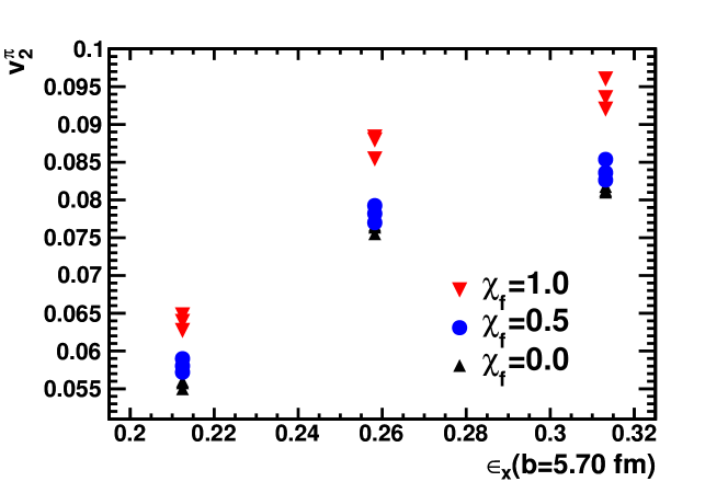
In contrast to the initial anisotropy of the shear tensor, the initial flow plays an important role in developing elliptic flow, parameterized here in terms of $\chi_{f}$, which is the fraction of the result in Equation 5.23 used in the initial state. This is evident in Figure 6.10 which shows the elliptic flow produced in all model runs for the 10-20% centrality bin, where the key difference from Figure 6.9 is that the symbols now indicate runs with the same initial flow. The model runs are well-ordered by the initial flow in every case with none of the zero initial flow output even within 10% of the full initial flow output. Even more tellingly, this persists over all types of initial conditions. This results in a combined uncertainty between the initial profile and the initial flow of almost 100% in the model prediction of the elliptic flow in this variable.

Figure 6.11: The transverse momentum weighted integrated anisotropic flow for the 20-30% centrality bin from the set of model runs described in the text. The solid marks are identical to those in Figure 6.9 now colored by initial flow ($\chi_{f}$) as described in Figure 6.10 and arbitrarily offset for clarity. Furthermore, open symbols are now included for model runs with double the viscosity ($\eta/s=0.32$) for the saturation models for initial conditions. The models runs with double the viscosity and the full amount of initial flow show the same amount of anisotropic flow as runs with the previous shear viscosity and no initial flow. This indicates that uncertainty in the initial flow results in 100% uncertainty in the value of the shear viscosity.

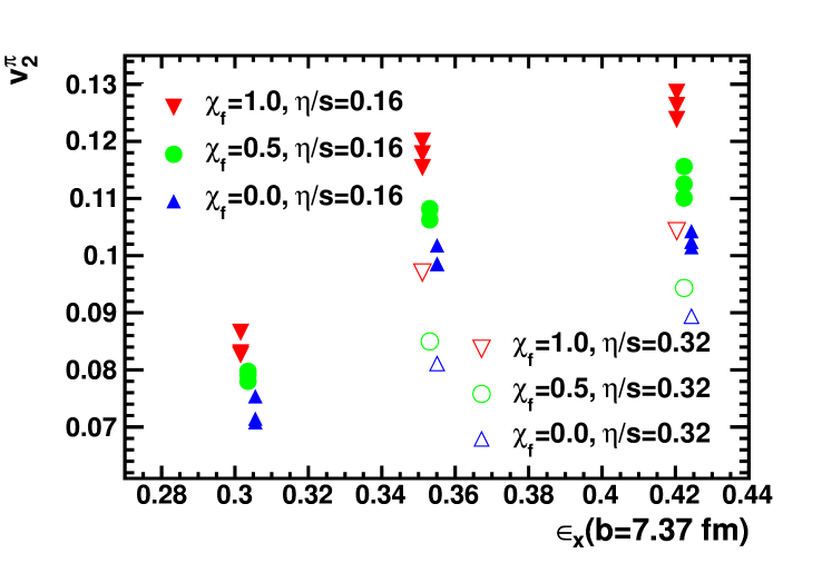
To see the effect of this uncertainty on the extraction of the shear viscosity near the phase transition, Figure 6.11 again shows all model runs distinguished by their initial flow. We’ve returned to the 20-30% centrality data in part to demonstrate that the effect is not unique to mid-central collisions which is very clear from the lower viscosity data presented. Furthermore, we now include additional runs with twice the original viscosity to confirm the findings from Figure 6.8 which showed that initial shape contributed a factor of roughly two to shear viscosity determination. Figure 6.11 confirms that the uncertainty in shear viscosity extraction due to the initial shape of the energy density is more than 100%. Runs with double the viscosity produce more elliptic for the screening and saturation initial conditions that remain larger than that seen with the default Glauber output, meaning that even more shear viscosity would have to be added to compensate for changing the initial conditions from a default Glauber model to a screening model. This uncertainty appears to be additive with the uncertainty contributed by uncertainty in the initial velocity profile as the spread in the results is not decreased as the viscosity is increased. Therefore even within a model that fixes the thermalization time, equation of state, temperature dependence of the shear viscosity, bulk viscosity, etc. one should expect a factor of three uncertainty in the extraction of the shear viscosity. This conclusion is based only on integrated elliptic flow data and it is possible that, for instance, the transverse momentum dependence of the elliptic flow could provide some additional resolving power though, as mentioned before, such a conclusion may depend more delicately upon details of the model.

6.2.2 Multiple Parameter Extraction

Efforts to understand the hydrodynamic parameter space is limited by the complexity of the hydrodynamic model itself and the uncertainties that are inherent to the choices in constructing one. This is underscored by the divisions between the several components of the model which are the initial condition to hydrodynamics, the hydrodynamic evolution, the hadronic cascade, and finally the analysis that calculates observables to be compared to experiment. Each of these contain many decisions that likely affect theoretical conclusions about the matter created in heavy ion collisions. For example, the initial condition to the hydrodynamic phase is not well understood and should be constrained experimentally. Therefore, one must investigate the sensitivity of any conclusion about the character of the matter to assumptions about the pre-equilibrium phase, that is, uncertainty about pre-equilibrium dynamics must be fully propagated to any extraction of properties of the the matter, like the shear viscosity or the equation of state. So while there is a great deal of experimental data to be analyzed, there are also a large number of parameters to be considered. Furthermore, the parameters do not necessarily have simple relationships to observables and many parameters may be important to the calculation of a single observable. The opposite is also true as a single parameter may affect many observables, and these effects may not be linear.

Model response throughout the parameter space was studied using the Markov Chain Monte Carlo (MCMC) method which takes random small steps through the parameter space, where the model emulator was used instead of evaluating the model at each point. The Metropolis-Hastings method of performing MCMC proceeds by always accepting steps to parameter settings that better describe the data and accepting worse settings with probability proportional to the ratio of the likelihoods, where the log-likelihood is proportional to the sum of the squares of the deviation from the experimental data. This means that after excluding a random walk near the first point chosen the set of parameter space points visited in the MCMC trace is proportional to the posterior likelihood – that is, the likelihood that a parameter setting is the true setting based on the model runs. This is not the only method of exploring model response to parameter variations, and other methods like gradient or Langevin search could be used to provide an estimate of the most likely point in parameter space; but they do not provide a direct estimate of the posterior distribution.

One difficulty of MCMC is that the model output must be known at every point in the parameter space. Unless the model is extremely fast to evaluate, it is necessary to be able to predict the output of the full model without evaluating it. In the simplest case, this could be done by interpolating linearly in each dimension between the model runs nearest to the point of interest. This has the benefit of simplicity but may miss important features of the space. Instead, we chose to emulate the aggregated observables of our hybrid hydrodynamic-cascade model using a Gaussian process [75]. This method assumes that the local correlation structure in parameter space is a multi-variate normal distribution and produces predictions of the mean and variance, essentially a prediction and the uncertainty in that prediction, at any point in the parameter space. To verify that the Gaussian process accurately infers model outputs, the predictions of the Gaussian process were tested against a withheld set of model runs which were all predicted to within an aggregate of three standard deviations over all model outputs. A more complete discussion of the Gaussian process model and its testing for this application are available as a pre-print at the time of writing [76].

The Gaussian process requires model output from the region of parameter space to be explored by the MCMC. Since we are interested in applications with a significant number of dimensions and the expected increase in required samplings scales exponentially with the number of dimensions, it is important that the sampling be done efficiently. The method used in this work which is Latin Hypercube sampling. which divides each dimension of the space into $n$ bins and then requires that exactly one sampling point to appear in each bin. The result is that there is no redundancy if a dimension turns out to be irrelevant and that many values of each parameter are present in the sampling.

Parameter	Description	Range
$(dE/dy)_{pp}$	The initial energy per rapidity in the diffuse limit compared to measured value in $pp$ collision	0.85–1.2
$\sigma_{\rm sat}$	This controls how saturation sets in as function of areal density of the target or projectile. In the wounded nucleon model it is assumed to be the free nucleon-nucleon cross section of 42 mb	30 mb–50 mb
$f_{wn}$	Determines the relative weight of the wounded-nucleon and saturation formulas for the initial energy density described in (6.2.2, 6.2)	0–1
$F_{\rm flow}$	Describes the strength of the initial flow as a fraction of the amount described in (5.23)	0.25–1.25
$\eta/s|_{T_{c}}$	Viscosity to entropy ratio for $T=170$ MeV	0 – 0.5
$\alpha$	Temperature dependence of $\eta/s$ for temperatures above freezeout, described in Equation 6.4	0 - 5

Table 6.1: Summary of model parameters. Six model parameters were varied. The first four describe the initial state being fed into the hydrodynamic module, and the last two describe the viscosity and its energy dependence.

In our first effort, we explore six parameters simultaneously. We chose four related to the initial condition and two related to the shear viscosity. The normalization of the energy density is essentially a required parameter to study plausible regions of parameter space and we chose to couch this in terms of the relationship to the total transverse energy produced in a minimum bias proton-proton collision at the same center of mass energy per nucleon. To test the importance of details of screening in the initial condition, we chose two related parameters that set the extent to which a screening model was used and the associated cross-section. The energy density within the model was therefore given by the set of equations given in terms of the Glauber thickness functions ($T_{A,B}$) by

$$\epsilon_{\rm wn}(x,y) = (dE/dy)_{pp}\frac{\sigma_{\rm nn}}{2\sigma_{\rm sat}}T_{A}(x,y)\left(1-\exp(-T_{B}(x,y)\sigma_{\rm sat})\right)$$

$$+(dE/dy)_{pp}\frac{\sigma_{\rm nn}}{2\sigma_{\rm sat}}T_{B}(x,y)\left(1-\exp(-T_{A}(x,y)\sigma_{\rm sat})\right),$$

$$\epsilon_{\rm sat}(x,y) = (dE/dy)_{pp}\frac{\sigma_{\rm nn}}{\sigma_{\rm sat.}}T_{\rm min}(x,y)\left(1-\exp(-T_{\rm max}(x,y)\sigma_{\rm sat})\right),$$ (6.2)

$$T_{\rm min} = \frac{2T_{A}T_{B}}{T_{A}+T_{B}},~{}~{}T_{\rm max}=(T_{A}+T_{B})/2.$$

The parameter to be varied within the model is $\sigma_{\rm sat}$ as $\sigma_{\rm nn}=42$ mb is the inelastic nucleon-nucleon cross-section and $(dE/dy)_{pp}=2.613$ GeV is the transverse energy per unit rapidity and is calculated directly from experimental data. The other two parameters are involved in the final calculation of the energy density from

$$\epsilon(x,y)=(\kappa/\tau)\left[f_{\rm wn}\epsilon_{\rm wn}(x,y)+(1-f_{\rm wn})\epsilon_{\rm sat}(x,y)\right]$$ (6.3)

where $\kappa$ is unity if the total transverse energy is the sum over the proton-proton collisions and increases in the total energy is larger, and $f_{\rm wn}$ determines the fraction of the energy distribution determined from the wounded nucleon scaling as opposed to screening scaling. The fourth parameter is the last related to the initial state and it sets the initial flow in the same way described in the previous subsection. The final two parameters related to the shear viscosity ratio and were the shear viscosity to entropy density ratio at the phase transition, $\left.\frac{\eta}{s}\right|_{T_{c}}$, with $T_{c}=170$ MeV being the same as the hydrodynamic freeze-out temperature, and the increase in the shear viscosity at higher temperatures that one expects from QCD arguments [49, 77, 50] moving away from the critical region,

$$\frac{\eta}{s}=\left.\frac{\eta}{s}\right|_{T_{c}}+\alpha\ln\left(\frac{T}{T_{c}}\right),$$ (6.4)

where $\alpha$ is this final parameter to be varied.

Our statistical method samples this parameter space somewhat minimally – $3^{6}=729$ points in the six dimensional space – at points chosen by Latin hypercube sampling. The produced particles were aggregated in the same way as the experimental data, for which we considered

• Low momentum pion yield at 0-5% and 20-30% centrality [9].

• Average transverse momentum for low momentum pions, kaons, and protons at each centrality [9].

• Three pion source radii from HBT at each centrality [78].

• Pion elliptic flow reduced by 10% to account for non-flow and with additional uncertainty to account for the lack of fluctuations in the initial conditions [79].

A Gaussian process was trained to emulate the aggregated model predictions and the space was sampling by MCMC as described above.

Among these, only HBT radii have not been discussed to this point. HBT radii measure the extent of the outgoing phase space cloud through two-particle momentum correlations. Experiments can measure the probability of detecting two particles at momenta $p_{a}$ and $p_{b}$ divided by the probability of finding particles of each momentum independently:

$$C^{ab}(\vec{P},\vec{q})=\frac{dN^{ab}/d^{3}p_{a}d^{3}p_{b}}{dN^{a}/d^{3}p_{a}\cdot dN^{b}/d^{3}p_{b}},$$ (6.5)

where $\vec{P}$ is the summed pair momentum and $\vec{q}$ is their relative momentum. In the limit that the observation of particle a is independent of the observation of particle b, $C^{ab}=1$. Instead, what is observed from heavy ion collisions is a rich correlation structure at moderate momentum. These correlations can be explained by a thermal source of finite size, $S^{ab}$, and a knowledge of the two-particle wave-function, $\phi$, by the Koonin-Pratt equation,

$$C^{ab}(\vec{P},\vec{q})=\int d^{3}r~{}S^{ab}(\vec{P},\vec{r})|\phi(\vec{q},\vec{r})|^{2}.$$ (6.6)

Typically, the source function is taken to be a Gaussian and is parameterized in terms of the radius in the outward, sideward, and longitudinal directions ($R_{o}$, $R_{s}$, $R_{l}$). The separation of the longitudinal radius is due to the expectation of differing dynamics in the direction. The outward radius is measured along the direction of the transverse momentum, and the sideward radius is orthogonal to the others. The difference between the outward radius and the sideward radius is then related to the explosiveness of the collision environment. Both the longitudinal radius and the explosiveness of the collision environment were poorly described by early, ideal hydrodynamic simulations of heavy ion collisions [22], which overestimated the longitudinal radius and explosiveness.

Figure 6.12: Pion, kaon, and proton transverse momentum spectra for the 5% most central collisions (above) and the 20-30% centrality bin (below). The red symbols are the experimental data as published and the green symbols are enhanced due to the absence of some chemical reactions in the gas calculation. The (blue) lines in the left panels show predictions from random model sampled uniformly from the entire model space, whereas the right side shows model runs selected weighted by the posterior likelihood distributions from the MCMC trace. This demonstrates that all model runs favored in the posterior distribution well describe the particle spectrum data.

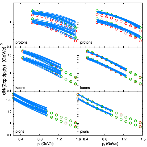
We compare twenty runs chosen randomly from the parameter space to twenty runs chosen from the MCMC trace. This corresponds to a weighted draw from the prior and posterior distributions respectively. The produced particle spectrum for each species and centrality is shown in Figure 6.12. The randomly chosen settings include many settings that can easily be excluded by the experimental data. Comparing this to those selected from the trace, we find all of the runs are in reasonable agreement with the data and none could easily be excluded on these merits given experimental uncertainties. We expect that many parameter settings will fit spectrum data but it is reassuring to find a region of parameter space that fits this data at a high level.

Figure 6.13: The anisotropic flow as a function of transverse momentum for pions. The (red) squares are experimental data from the STAR collaboration. The twenty (blue) lines are model runs in each panel; in the top panel they are chosen via uniform sampling of the parameter space while in the bottom panel they are taken randomly from the MCMC trace which samples more likely regions more heavily. The runs from the MCMC trace are considerably closer to the experimental data but note that the posterior distribution contains many settings that do not describe the anisotropic data with high precision.

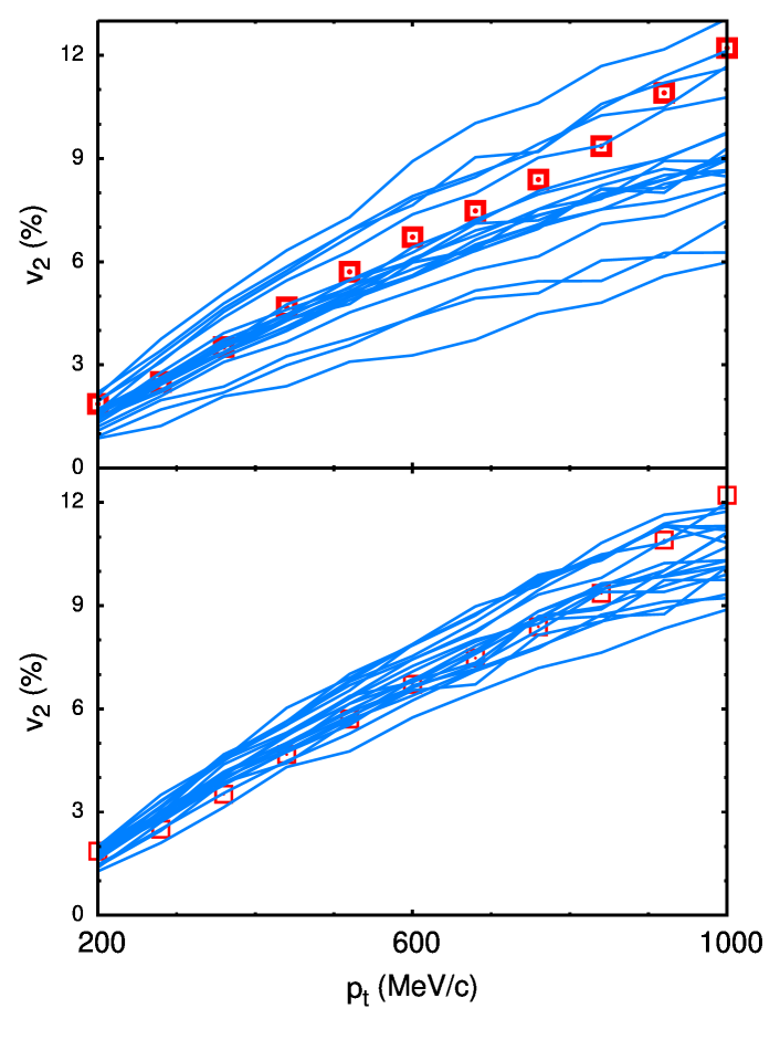
For the pion elliptic flow output and data, Figure 6.13 shows the same model runs selected from the prior and posterior distributions. Again the prior distribution contains many runs that deviate significantly from the experimental data, whereas the posterior distribution is clustered around the data. Here the deviation is larger than in the case of the spectrum which is at least in part due to the increased uncertainty from the experiment which was 12% [17, 18] as opposed to the multiplicities which had uncertainties of 6% and the average transverse momentum which had uncertainties of only 3% [9, 2]. This is larger than the experimental uncertainties since we do not include initial condition fluctuations. Also note that there are some systematic differences in shape between the model runs and the experimental data, with the model runs over-predicting $v_{2}$ at lower momentum and under-predicting it at high momentum. This is in contrast to Figures 6.7 and 6.8 which showed the opposite issue, though there are parameter differences between those from the posterior distribution here and those taken in that study including the freeze-out temperature which is higher in this case by 5 MeV.

Figure 6.14: Pion HBT radii as a function of transverse momentum for central (red circles) and mid-central (blue squares). In the left panel, the lines are from model runs with parameters drawn from the flat prior distribution, whereas in the right panel, the parameter settings are weighted by the posterior distribution. The parameter settings from the posterior distribution exhibit more explosiveness as evidenced by the increased $R_{o}/R_{S}$ ratio and more precise predictions in general that describe the experimental data except for in the lowest momentum bin.

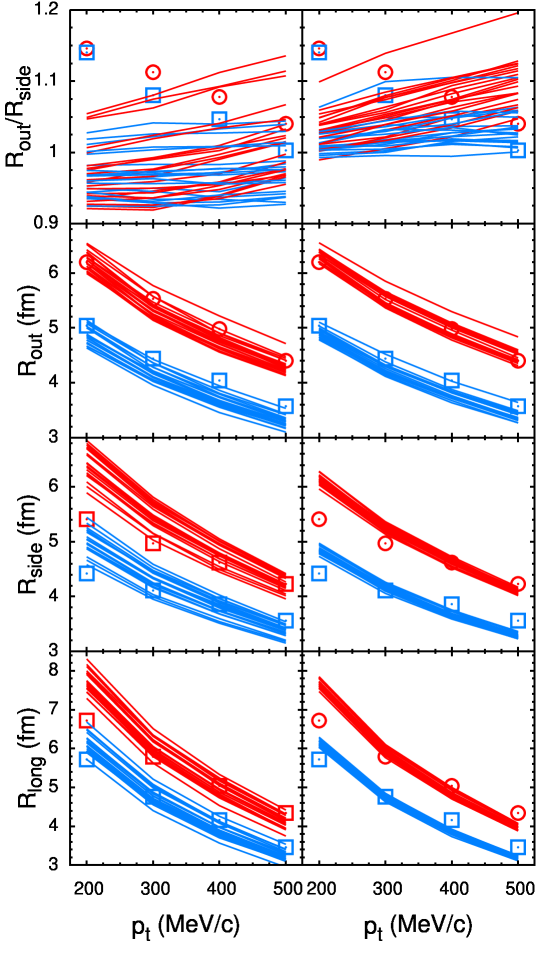
The HBT radii were also reproduced well by the runs pulled from the posterior distribution as evidenced in Figure 6.14. The model runs drawn from the prior distribution show more spread and tend to overestimate the sideward radius and underestimate the outward radius. For runs from the posterior distribution, the outward radius is described well at all momenta, while the other radii are overestimated in the lowest momentum bin. It is concerning that the momentum dependence of the sideward radius appears to be too dramatic, but the source of this discrepancy is not understood.

Figure 6.15: Parameter space density plots for the Markov Chain Monte Carlo trace run over the Gaussian process emulation of the hybrid model. On-diagonal plots show the density projecting out all five remaining variables while the off-diagonal plots show the two-dimensional density distribution projecting out the four remaining variables. The one-dimensional plots show that the most likely parameter sets feature a small but non-zero value of the shear viscosity, almost no increase to the shear viscosity at high temperatures, small pre-equilibrium flow, and a density distribution more like wounded nucleon than the screening model. The two-dimensional plots show how these conclusions depend on one another. As expected, more eccentric initial conditions from the screening model lead runs with a higher value of the shear viscosity to better agree with the data. The sum of the shear viscosity in the critical region and the slope of the shear viscosity above the critical region appears well constrained; and likewise, the difference between the saturation cross-section and the energy density normalization appears well-constrained.

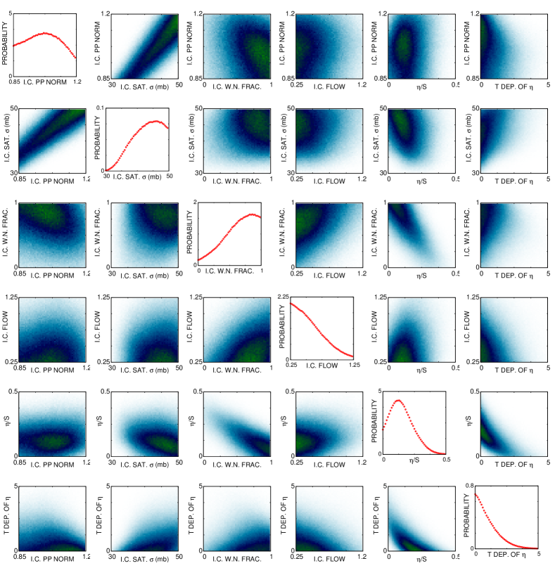
Displaying the posterior distribution itself is a difficult task as the posterior distribution is a six-dimensional density distribution. Our method is to take all possible projections of the distribution in one- and two-dimensions and this is shown for our space in Figure 6.15. If one begins by looking at the one-dimensional projections, it appears that both parameters related to the shear viscosity ($\eta/s$ and T_DEP_OF_$\eta$) are reduced to a fraction of their tested range, while the normalization (I.C._PP_ NORM) and the saturation cross-section (I.C._SAT._ $\sigma$ (mb)) are barely constrained at all. However, if one moves to the two-dimensional plots we see that this is only because of our choice of variables and that a linear combination of the normalization and the saturation cross-section (roughly their difference) is constrained – presumably by the multiplicities – whereas the orthogonal combination (their sum) is only somewhat constrained. The physical explanation of this is not so clear but perhaps a slow change in the centrality scaling of the multiplicity or the initial eccentricity due to changing the saturation cross-section.

We find other expected parameter behaviors in the correlation plots of Figure 6.15. For instance, the model better describes the data when shear viscosity at the critical temperature is larger for models containing saturation than for the wounded nucleon picture due to larger eccentricities. Also the optimal shear viscosity at the critical temperature is inversely related with the slope of the shear viscosity at higher temperatures. This suggests that the model output is sensitive to the average shear viscosity in the region near or above the critical temperature. It is surprising then that initial conditions involving more saturation, or more initial eccentricity, do not support a larger high temperature slope but rather a lower one. This implies a tension in the model output that is not immediately clear but warrants future investigation. The conclusion that quark matter has small shear viscosity seems to be robust. Just how small the shear viscosity is appears to be correlated with other parameters including the temperature dependence of the shear viscosity but also the details of the nucleon screening model. The lack of dependence on the initial flow is in contrast to our results from the previous subsection. Given that elliptic flow increases with increasing pre-equilibrium flow and decreases with increasing shear viscosity, one would expect that elliptic flow would only be sensitive to the difference between these parameters. This suggests that other experimental data is breaking this expected relationship but the source of this is not well understood. Another important future investigation might determine which experimental data underpin this conclusion and attempt to identify other model parameters that could compromise it.

Also of interest is that the posterior distribution dependence on normalization is weak except when varying the saturation cross-section. This suggests that future studies could avoid sampling in that parameter by locating the normalization that reproduces experimental multiplicities as done in the previous subsection. This is attractive because multiplicities require less than one hundred cascade events to calculate accurately at the one percent level in contrast to the four thousand events used to generate each point in parameter space sampled, in addition to reducing the dimensionality of the parameter space.

6.3 Concluding Remarks

The broad conclusion of this work is that adding the non-trivial aspects of the longitudinal expansions to viscous hydrodynamic modeling does not dramatically affect conclusions about the matter formed in heavy ion collisions. We arrived at this conclusion by investigating the matter in the hydrodynamic phase and noting that the flow velocity shows no change when fully including the longitudinal expansion, as seen in Figure 6.3. As the flow profile is the driver of elliptic flow, conclusions about the dynamics of the hot matter drawn from two dimensional simulations are trustworthy. While Figure 6.4 shows a decrease in the predicted source lifetime, the most dramatic effect of this is to decrease the longitudinal source size. This proves a nice solution to an existing tension between theoretical models and the experimental data. These conclusions are based on simulations done for collisions with beam energy of $\sqrt{s_{NN}}=200$ GeV and are expected to hold for larger beam energies, though they would need to be revisited for smaller beam energies.

This does not imply that there is no reason to pursue further three dimensional viscous models. Instead it means that it is not necessary to model midrapidity data at the highest RHIC energy, unless one pursues accuracy at better than the 5% level. Even at small longitudinal rapidity, more experimental data become accessible to an extended version of our model, including directed flow due to non-zero impact parameter and the associated angular momentum of the source. Attempts to include the effects of non-zero angular momentum in the initial condition [80] within the current version of the model have demonstrated persistent instability that have frustrated attempts to study its possible influence at midrapidity. Schematic changes to the integration of the basic hydrodynamic equations may be necessary to undertake such a study.

These upgrades would make other effects available for study as well, for instance, a method that is stable against shocks would allow one to study the role of fluctuations. In the model described here, hydrodynamic modeling is a small fraction of the computational time compared to the generation, manipulation and analysis of the particles within the resonance gas model. Assuming that the described changes do not significantly alter this balance, one can imagine running around fifty hydrodynamic events per centrality bin at a cost of less than a factor of two in the run time. This would allow investigation of fluctuation data including average transverse momentum fluctuations and elliptic flow fluctuations both with and without boost invariance.

Other features of particle production away from midrapidity include the effects of finite baryon number and the development of elliptic flow away from midrapidity. In this model, the finite baryon number from the protons and neutrons in the original nuclei is carried away. While the nuclei recede rapidly, baryon current diffuses toward midrapidity and manifests itself as an imbalance between the number of protons and anti-protons at midrapidity. This baryon current would be a necessary feature of any model attempting to investigate effects away from midrapidity as it seems likely to affect other important observables like elliptic flow. For instance, if the matter has more heavy baryons, then at the same energy density the pressure is reduced, due to a decrease in the mean velocity, and flow should develop more slowly. Since elliptic flow falls more rapidly than multiplicity as a function of pseudorapidity, this may be an interesting phenomenon and could provide consistency checks on the initial conditions that underpin hydrodynamic models.

While there is much to be gained from continued study of three-dimensional viscous hydrodynamic models, there is still quite a lot to be learned about two-dimensional models as well. While the six-dimensional parameter study shown in Figure 6.15 demonstrates that we understand some of the experimental constraints on model parameters, the full set of parameters is very large and many important parameters have yet to be explored. The equation of state calculated by lattice QCD seems to be a theoretical triumph especially given its agreement with the expectations of the hadron resonance gas near the phase transition. However, it remains unknown whether or not experimental data gathered from heavy ion collisions support the conclusion that equilibrium dynamics of the quark-gluon plasma are well described by the equation of state predicted by lattice QCD. Direct experimental evidence for lattice QCD would be a massive triumph and remains an important goal of the field of relativistic heavy ion collisions.

References

- Adams et al. [2003] J. Adams, et al. (STAR Collaboration), Evidence from d + Au measurements for final state suppression of high p(T) hadrons in Au+Au collisions at RHIC, Phys.Rev.Lett. 91 (2003) 072304.
- Abelev et al. [2009] B. Abelev, et al. (STAR Collaboration), Systematic Measurements of Identified Particle Spectra in Au and Au+Au Collisions from STAR, Phys.Rev. C79 (2009) 034909.
- Kolb [2002] P. F. Kolb, Early Thermalization and Hydrodynamic Expansion in Nuclear Collisions at RHIC, Ph.D. thesis, 2002.
- Adare et al. [2007] A. Adare, et al. (PHENIX Collaboration), Scaling properties of azimuthal anisotropy in Au+Au and Cu+Cu collisions at s(NN) = 200-GeV, Phys.Rev.Lett. 98 (2007) 162301.
- Bearden et al. [2005] I. Bearden, et al. (BRAHMS Collaboration), Charged meson rapidity distributions in central Au+Au collisions at s(NN)**(1/2) = 200-GeV, Phys.Rev.Lett. 94 (2005) 162301.
- Borsanyi et al. [2010] S. Borsanyi, G. Endrodi, Z. Fodor, A. Jakovac, S. D. Katz, et al., The QCD equation of state with dynamical quarks, JHEP 1011 (2010) 077.
- Huovinen and Petersen [2012] P. Huovinen, H. Petersen, Particlization in hybrid models (2012).
- Drescher et al. [2006] H.-J. Drescher, A. Dumitru, A. Hayashigaki, Y. Nara, The Eccentricity in heavy-ion collisions from color glass condensate initial conditions, Phys.Rev. C74 (2006) 044905.
- Adler et al. [2004] S. Adler, et al. (PHENIX Collaboration), Identified charged particle spectra and yields in Au+Au collisions at S(NN)**1/2 = 200-GeV, Phys.Rev. C69 (2004) 034909.
- Bass et al. [1999] S. Bass, M. Bleicher, W. Cassing, A. Dumitru, H. Drescher, et al., Last call for RHIC predictions, Nucl.Phys. A661 (1999) 205–260.
- Adamczyk et al. [2012] L. Adamczyk, et al. (STAR collaboration), Inclusive charged hadron elliptic flow in Au + Au collisions at = 7.7 - 39 GeV, Phys.Rev. C86 (2012) 054908.
- Adcox et al. [2002] K. Adcox, et al. (PHENIX Collaboration), Suppression of hadrons with large transverse momentum in central Au+Au collisions at = 130-GeV, Phys.Rev.Lett. 88 (2002) 022301.
- Adams et al. [2005] J. Adams, et al. (STAR Collaboration), Distributions of charged hadrons associated with high transverse momentum particles in pp and Au + Au collisions at s(NN)**(1/2) = 200-GeV, Phys.Rev.Lett. 95 (2005) 152301.
- Adler et al. [2003] C. Adler, et al. (STAR Collaboration), Disappearance of back-to-back high hadron correlations in central Au+Au collisions at = 200-GeV, Phys.Rev.Lett. 90 (2003) 082302.
- Ackermann et al. [2001] K. Ackermann, et al. (STAR Collaboration), Elliptic flow in Au + Au collisions at (S(NN))**(1/2) = 130 GeV, Phys.Rev.Lett. 86 (2001) 402–407.
- Adler et al. [2003] S. Adler, et al. (PHENIX Collaboration), Elliptic flow of identified hadrons in Au+Au collisions at s(NN)**(1/2) = 200-GeV, Phys.Rev.Lett. 91 (2003) 182301.
- Abelev et al. [2008] B. Abelev, et al. (STAR Collaboration), Centrality dependence of charged hadron and strange hadron elliptic flow from s(NN)**(1/2) = 200-GeV Au + Au collisions, Phys.Rev. C77 (2008) 054901.
- Afanasiev et al. [2009] S. Afanasiev, et al. (PHENIX Collaboration), Systematic Studies of Elliptic Flow Measurements in Au+Au Collisions at s**(1/2) = 200-GeV, Phys.Rev. C80 (2009) 024909.
- Armesto et al. [2012] N. Armesto, B. Cole, C. Gale, W. A. Horowitz, P. Jacobs, et al., Comparison of Jet Quenching Formalisms for a Quark-Gluon Plasma ’Brick’, Phys.Rev. C86 (2012) 064904.
- Kolb and Heinz [2003] P. F. Kolb, U. W. Heinz, Hydrodynamic description of ultrarelativistic heavy ion collisions (2003).
- Adams et al. [2005] J. Adams, et al. (STAR Collaboration), Experimental and theoretical challenges in the search for the quark gluon plasma: The STAR Collaboration’s critical assessment of the evidence from RHIC collisions, Nucl.Phys. A757 (2005) 102–183.
- Heinz and Kolb [2002] U. W. Heinz, P. F. Kolb, Two RHIC puzzles: Early thermalization and the HBT problem (2002).
- Pratt [2009] S. Pratt, Resolving the HBT Puzzle in Relativistic Heavy Ion Collision, Phys.Rev.Lett. 102 (2009) 232301.
- Schmidt [2006] C. Schmidt, Lattice QCD at finite density, PoS LAT2006 (2006) 021.
- Huovinen and Petreczky [2011] P. Huovinen, P. Petreczky, Equation of state at finite baryon density based on lattice QCD, J.Phys. G38 (2011) 124103.
- Song and Heinz [2008] H. Song, U. W. Heinz, Causal viscous hydrodynamics in 2+1 dimensions for relativistic heavy-ion collisions, Phys.Rev. C77 (2008) 064901.
- Luzum and Romatschke [2008] M. Luzum, P. Romatschke, Conformal Relativistic Viscous Hydrodynamics: Applications to RHIC results at s(NN)**(1/2) = 200-GeV, Phys.Rev. C78 (2008) 034915.
- Dusling and Teaney [2008] K. Dusling, D. Teaney, Simulating elliptic flow with viscous hydrodynamics, Phys.Rev. C77 (2008) 034905.
- Bjorken [1983] J. Bjorken, Highly Relativistic Nucleus-Nucleus Collisions: The Central Rapidity Region, Phys.Rev. D27 (1983) 140–151.
- Bazavov et al. [2009] A. Bazavov, T. Bhattacharya, M. Cheng, N. Christ, C. DeTar, et al., Equation of state and QCD transition at finite temperature, Phys.Rev. D80 (2009) 014504.
- Huang [1987] K. Huang, Statistical Mechanics, 2 ed., Wiley, 1987.
- Romatschke [2010] P. Romatschke, New Developments in Relativistic Viscous Hydrodynamics, Int.J.Mod.Phys. E19 (2010) 1–53.
- Betz et al. [2009] B. Betz, D. Henkel, D. Rischke, From kinetic theory to dissipative fluid dynamics, Prog.Part.Nucl.Phys. 62 (2009) 556–561.
- Huovinen and Molnar [2009] P. Huovinen, D. Molnar, The Applicability of causal dissipative hydrodynamics to relativistic heavy ion collisions, Phys.Rev. C79 (2009) 014906.
- Pratt [2008] S. Pratt, Formulating viscous hydrodynamics for large velocity gradients, Phys.Rev. C77 (2008) 024910.
- Muronga [2002] A. Muronga, Second order dissipative fluid dynamics for ultrarelativistic nuclear collisions, Phys.Rev.Lett. 88 (2002) 062302.
- Baier et al. [2008] R. Baier, P. Romatschke, D. T. Son, A. O. Starinets, M. A. Stephanov, Relativistic viscous hydrodynamics, conformal invariance, and holography, JHEP 0804 (2008) 100.
- Muronga [2007a] A. Muronga, Relativistic Dynamics of Non-ideal Fluids: Viscous and heat-conducting fluids. I. General Aspects and 3+1 Formulation for Nuclear Collisions, Phys.Rev. C76 (2007a) 014909.
- Muronga [2007b] A. Muronga, Relativistic Dynamics of Non-ideal Fluids: Viscous and heat-conducting fluids. II. Transport properties and microscopic description of relativistic nuclear matter, Phys.Rev. C76 (2007b) 014910.
- Grad [1949] H. Grad, Commun. Pure App. Math 2 (1949) 381.
- Baier et al. [2006] R. Baier, P. Romatschke, U. A. Wiedemann, Dissipative hydrodynamics and heavy ion collisions, Phys.Rev. C73 (2006) 064903.
- Huovinen and Petreczky [2010] P. Huovinen, P. Petreczky, QCD Equation of State and Hadron Resonance Gas, Nucl.Phys. A837 (2010) 26–53.
- Press et al. [1992] W. H. Press, S. A. Teukolsky, W. T. Vetterling, B. P. Flannery, Numerical recipes in C (2nd ed.): the art of scientific computing, Cambridge University Press, New York, NY, USA, 1992.
- Paech and Pratt [2006] K. Paech, S. Pratt, Origins of bulk viscosity in relativistic heavy ion collisions, Phys.Rev. C74 (2006) 014901.
- Weinberg [1995] S. Weinberg, The Quantum Theory of Fields (Volume 1), 1 ed., Cambridge University Press, 1995. URL: http://www.worldcat.org/isbn/0521550017.
- Prakash et al. [1993] M. Prakash, M. Prakash, R. Venugopalan, G. Welke, Nonequilibrium properties of hadronic mixtures, Phys.Rept. 227 (1993) 321–366.
- Song et al. [2011] H. Song, S. A. Bass, U. Heinz, Viscous QCD matter in a hybrid hydrodynamic+Boltzmann approach, Phys.Rev. C83 (2011) 024912.
- Niemi et al. [2012] H. Niemi, G. Denicol, P. Huovinen, E. Molnar, D. Rischke, Influence of a temperature-dependent shear viscosity on the azimuthal asymmetries of transverse momentum spectra in ultrarelativistic heavy-ion collisions, Phys.Rev. C86 (2012) 014909.
- Csernai et al. [2006] L. P. Csernai, J. Kapusta, L. D. McLerran, On the Strongly-Interacting Low-Viscosity Matter Created in Relativistic Nuclear Collisions, Phys.Rev.Lett. 97 (2006) 152303.
- Huot et al. [2007] S. C. Huot, S. Jeon, G. D. Moore, Shear viscosity in weakly coupled N = 4 super Yang-Mills theory compared to QCD, Phys.Rev.Lett. 98 (2007) 172303.
- Boris and Book [1973] J. Boris, D. Book, J. Comput. Phys. 11 (1973) 38.
- Kurganov and Tadmor [2000] A. Kurganov, E. Tadmor, Journal of Computational Physics 160 (2000) 214.
- Pratt and Torrieri [2010] S. Pratt, G. Torrieri, Coupling Relativistic Viscous Hydrodynamics to Boltzmann Descriptions, Phys.Rev. C82 (2010) 044901.
- Holopainen and Huovinen [2012] H. Holopainen, P. Huovinen, Dynamical Freeze-out in Event-by-Event Hydrodynamics, J.Phys.Conf.Ser. 389 (2012) 012018.
- Holopainen et al. [2011] H. Holopainen, H. Niemi, K. J. Eskola, Event-by-event hydrodynamics and elliptic flow from fluctuating initial state, Phys.Rev. C83 (2011) 034901.
- Cooper and Frye [1974] F. Cooper, G. Frye, Phys. Rev. D 10 (1974) 186.
- William E. Lorensen [1987] H. E. C. William E. Lorensen, Marching cubes: A high resolution 3d surface construction algorithm, Computer Graphics 21 (1987) 4.
- Miller et al. [2007] M. L. Miller, K. Reygers, S. J. Sanders, P. Steinberg, Glauber modeling in high energy nuclear collisions, Ann.Rev.Nucl.Part.Sci. 57 (2007) 205–243.
- Kolb et al. [2001] P. Kolb, U. W. Heinz, P. Huovinen, K. Eskola, K. Tuominen, Centrality dependence of multiplicity, transverse energy, and elliptic flow from hydrodynamics, Nucl.Phys. A696 (2001) 197–215.
- Kharzeev et al. [2004] D. Kharzeev, E. Levin, M. Nardi, QCD saturation and deuteron nucleus collisions, Nucl.Phys. A730 (2004) 448–459.
- McLerran and Venugopalan [1994] L. D. McLerran, R. Venugopalan, Computing quark and gluon distribution functions for very large nuclei, Phys.Rev. D49 (1994) 2233–2241.
- Lappi and Venugopalan [2006] T. Lappi, R. Venugopalan, Universality of the saturation scale and the initial eccentricity in heavy ion collisions, Phys.Rev. C74 (2006) 054905.
- Iancu and Venugopalan [2003] E. Iancu, R. Venugopalan, The Color glass condensate and high-energy scattering in QCD (2003).
- Drescher and Nara [2007] H.-J. Drescher, Y. Nara, Effects of fluctuations on the initial eccentricity from the Color Glass Condensate in heavy ion collisions, Phys.Rev. C75 (2007) 034905.
- Kolb et al. [2000] P. F. Kolb, J. Sollfrank, U. W. Heinz, Anisotropic transverse flow and the quark hadron phase transition, Phys.Rev. C62 (2000) 054909.
- Hirano and Tsuda [2003] T. Hirano, K. Tsuda, Collective flow and HBT radii from a full 3-D hydrodynamic model with early chemical freezeout, Nucl.Phys. A715 (2003) 821–824.
- Schenke et al. [2010] B. Schenke, S. Jeon, C. Gale, (3+1)D hydrodynamic simulation of relativistic heavy-ion collisions, Phys.Rev. C82 (2010) 014903.
- Vredevoogd and Pratt [2009] J. Vredevoogd, S. Pratt, Universal Flow in the First Stage of Relativistic Heavy Ion Collisions, Phys.Rev. C79 (2009) 044915.
- Teaney et al. [2001] D. Teaney, J. Lauret, E. Shuryak, A hydrodynamic description of heavy ion collisions at the sps and rhic (2001).
- Heinz and Kolb [2002] U. W. Heinz, P. F. Kolb, Early thermalization at RHIC, Nucl.Phys. A702 (2002) 269–280.
- Shen and Heinz [2012] C. Shen, U. Heinz, Collision Energy Dependence of Viscous Hydrodynamic Flow in Relativistic Heavy-Ion Collisions, Phys.Rev. C85 (2012) 054902.
- Song and Heinz [2008] H. Song, U. Heinz, Causal viscous hydrodynamics in 2 + 1 dimensions for relativistic heavy-ion collisions, Phys. Rev. C 77 (2008) 064901.
- Dusling et al. [2010] K. Dusling, G. D. Moore, D. Teaney, Radiative energy loss and v(2) spectra for viscous hydrodynamics, Phys.Rev. C81 (2010) 034907.
- Kovtun et al. [2005] P. Kovtun, D. Son, A. Starinets, Viscosity in strongly interacting quantum field theories from black hole physics, Phys.Rev.Lett. 94 (2005) 111601.
- Rasmussen [2006] C. E. Rasmussen, Gaussian processes for machine learning, MIT Press, 2006.
- Novak et al. [2013] J. Novak, K. Novak, S. Pratt, C. Coleman-Smith, R. Wolpert, Determining Fundamental Properties of Matter Created in Ultrarelativistic Heavy-Ion Collisions (2013).
- York and Moore [2009] M. A. York, G. D. Moore, Second order hydrodynamic coefficients from kinetic theory, Phys.Rev. D79 (2009) 054011.
- Abelev et al. [2009] B. Abelev, et al. (STAR Collaboration), Pion Interferometry in Au+Au and Cu+Cu Collisions at RHIC, Phys.Rev. C80 (2009) 024905.
- Adams et al. [2005] J. Adams, et al. (STAR Collaboration), Azimuthal anisotropy in Au+Au collisions at s(NN)**(1/2) = 200-GeV, Phys.Rev. C72 (2005) 014904.
- Adil and Gyulassy [2005] A. Adil, M. Gyulassy, 3D jet tomography of twisted strongly coupled quark gluon plasmas, Phys.Rev. C72 (2005) 034907.