Copula Calibration

Abstract

We propose notions of calibration for probabilistic forecasts of general multivariate quantities. Probabilistic copula calibration is a natural analogue of probabilistic calibration in the univariate setting. It can be assessed empirically by checking for the uniformity of the copula probability integral transform (CopPIT), which is invariant under coordinate permutations and coordinatewise strictly monotone transformations of the predictive distribution and the outcome. The CopPIT histogram can be interpreted as a generalization and variant of the multivariate rank histogram, which has been used to check the calibration of ensemble forecasts. Climatological copula calibration is an analogue of marginal calibration in the univariate setting. Methods and tools are illustrated in a simulation study and applied to compare raw numerical model and statistically postprocessed ensemble forecasts of bivariate wind vectors.

1 Introduction

The past two decades have witnessed major developments in the scientific approach to forecasting, in that probabilistic forecasts, which take the form of probability distributions over future quantities and events, have been replacing single-valued point forecasts in a wealth of applications (Gneiting and Katzfuss, 2014). The goal in probabilistic forecasting is to maximize the sharpness of the predictive probability distributions subject to calibration (Gneiting et al., 2007). Calibration concerns the statistical compatibility between the predictive distributions and the realizing observations; in a nutshell, the observations are supposed to be indistinguishable from random numbers drawn from the predictive distributions.

For probabilistic forecasts of univariate quantities various types of calibration have been established (Gneiting and Ranjan, 2013). In particular, a forecast is probabilistically calibrated if its probability integral transform (PIT), i.e., the value of the predictive cumulative distribution function at the realizing observation, is uniformly distributed. Accordingly, empirical checks for the uniformity of histograms of PIT values have formed a cornerstone of density forecast evaluation (Dawid, 1984; Diebold et al., 1998; Gneiting et al., 2007).

In this paper we introduce notions of calibration for probabilistic forecasts of multivariate quantities and propose tools for empirical calibration checks in such settings, as recently called for in hydrologic and meteorological applications (Schaake et al., 2010; Pinson, 2013; Schefzik et al., 2013). In Section 2 we study a natural multivariate extension of the univariate PIT that is invariant under coordinate permutations and coordinatewise strictly monotone transformations of the predictive distribution and the realizing observation, namely, the copula probability integral transform (CopPIT). Probabilistic copula calibration can be assessed empirically by checking the uniformity of the CopPIT histogram, which can be viewed as a generalization and variant of the multivariate rank histogram proposed by Gneiting et al. (2008). Furthermore, we introduce the notion of climatological copula calibration, which is an analogue of marginal calibration in the univariate setting. The strengths of these notions and tools include their ease of interpretability and their applicability to both density and ensemble forecasts.

In Section 3 we employ CopPIT histograms in a simulation study, and in Section 4 we use them to compare raw numerical model and statistically postprocessed ensemble forecasts of bivariate wind vectors over Germany. The paper ends with a discussion in Section 5.

2 Multivariate notions of calibration

We introduce the copula probability integral transform (CopPIT) and the notions of probabilistic copula calibration and climatological copula calibration within the prediction space setting of Gneiting and Ranjan (2013). Throughout, we identify a probability measure on $\mathbb{R}^{d}$ with its cumulative distribution function (CDF).

The Kendall distribution function $\mathcal{K}_{H}$ of a probability measure or CDF $H$ on $\mathbb{R}^{d}$ is defined as

$$\mathcal{K}_{H}(w)=\mathrm{pr}\{H(X)\leq w\}\quad\mbox{for}\quad w\in[0,1],$$

where the random vector $X$ has distribution $H$. It is well known that if $d=1$ and $H$ is continuous then $\mathcal{K}_{H}$ corresponds to a uniform distribution on $[0,1]$. In dimension $d>1$, the Kendall distribution depends only on the copula of the probability measure $H$ and generally it is not uniform (Barbe et al., 1996). In fact, for any CDF $K$ on $[0,1]$ with $K(w)\geq w$ for $w\in[0,1]$ and any integer $d>1$, there exists a probability measure $H$ on $\mathbb{R}^{d}$ such that $\mathcal{K}_{H}=K$ (Nelsen et al., 2003; Genest et al., 2011).

2.1 Probabilistic and climatological copula calibration

As noted, we work in the prediction space setting introduced by Gneiting and Ranjan (2013). Specifically, let $(\Omega,\mathcal{A},\mathbb{Q})$ be a probability space. Let $Y$ be an $\mathbb{R}^{d}$-valued random vector on $\Omega$, and let $H$ be a $d$-variate CDF-valued random quantity that is measurable with respect to some sub $\sigma$-algebra $\mathcal{A}_{0}\subseteq\mathcal{A}$. Furthermore, let the random variable $V$ be uniformly distributed on the unit interval $[0,1]$ and independent of $Y$ and $\mathcal{A}_{0}$.

The CDF-valued random quantity $H$ provides an $\mathcal{A}_{0}$-measureable predictive probability measure for the $\mathbb{R}^{d}$-valued outcome $Y$. It is said to be ideal relative to $\mathcal{A}_{0}$ if it equals the conditional law of $Y$ given $\mathcal{A}_{0}$, which we denote by $H=\mathcal{L}(Y|\mathcal{A}_{0})$. Thus, an ideal forecast honors the information in the sub $\sigma$-algebra $\mathcal{A}_{0}\subseteq\mathcal{A}$ to the full extent possible. For a function $f$ on the real line, we use the notation $f(y-)=\lim_{x\uparrow y}f(x)$ to denote the left-hand limit, if it exists.

Definition 2.1 (CopPIT).

In the prediction space setting, the random variable

$$U_{H}=\mathcal{K}_{H}\{H(Y)-\}+V\left[\mathcal{K}_{H}\{H(Y)\}-\mathcal{K}_{H}\{H(Y)-\}\right]$$ (1)

is the copula probability integral transform (CopPIT) of the CDF-valued random quantity $H$.

If $T$ is a deterministic coordinatewise strictly monotone transformation on $\mathbb{R}^{d}$, i.e.,

$$T(x_{1},\ldots,x_{d})=\left(T_{1}(x_{1}),\ldots,T_{d}(x_{d})\right)$$

where the mappings $T_{1},\ldots,T_{d}$ are real-valued and strictly increasing, the distribution of $U_{H}$ for the probabilistic forecast $H$ and the outcome $Y$ is the same as that of $U_{H\circ T^{-1}}$ for the probabilistic forecast $H\circ T^{-1}$ and the outcome $T(Y)$. The distribution of $U_{H}$ also is invariant under coordinate permutations. An interesting open question is for the largest class of transformations under which this invariance holds, with the class of the locally orientation preserving functions being a candidate.

Definition 2.2.

The forecast $H$ is probabilistically copula calibrated if its CopPIT is uniformly distributed on the unit interval.

Probabilistic copula calibration can be viewed as a multivariate generalization of the notion of probabilistic calibration in the univariate case. In the prediction space setting, let $F$ be a univariate CDF-valued random quantity for the real-valued outcome $Y$. Gneiting and Ranjan (2013, Definition 2.6) define $F$ to be probabilistically calibrated if

$$U_{F}=F(Y-)+V\{F(Y)-F(Y-)\}$$ (2)

is standard uniformly distributed. If the dimension is $d=1$ then equation (1) is the same as equation (2).

Definition 2.3.

The forecast $H$ is climatologically copula calibrated if

$$\mathbb{Q}\{H(Y)\leq w\}=\mathbb{E}_{\hskip 0.56905pt\mathbb{Q}}\{\mathcal{K}_{H}(w)\}\quad\mbox{for}\quad w\in[0,1].$$ (3)

The concept of climatological copula calibration can be interpreted as marginal calibration of the Kendall distribution, where marginal calibration refers to the univariate prediction space setting, as follows (Gneiting and Ranjan, 2013, Definition 2.6). If $F$ is a univariate CDF-valued random quantity for the real-valued outcome $Y$, then it is marginally calibrated if $\mathbb{Q}(Y\leq y)=\mathbb{E}_{\hskip 0.56905pt\mathbb{Q}}\{F(y)\}$ for $y\in\mathbb{R}$.

The following result justifies the quest for probabilistically and climatologically copula calibrated probabilistic forecasts in practical settings.

Theorem 2.1.

If the forecast $H$ is ideal with respect to the $\sigma$-algebra $\mathcal{A}_{0}$, then it is both probabilistically and climatologically copula calibrated.

Proof.

Suppose that $H=\mathcal{L}(Y|\mathcal{A}_{0})$ and let $w\in[0,1]$. Then

$$\mathbb{Q}\{H(Y)\leq w\}=\mathbb{E}_{\hskip 0.56905pt\mathbb{Q}}\,\mathbb{E}_{\hskip 0.56905pt\mathbb{Q}}\left[\mathbbm{1}\{H(Y)\leq w\}|\mathcal{A}_{0}\right]=\mathbb{E}_{\hskip 0.56905pt\mathbb{Q}}\{\mathcal{K}_{H}(w)\},$$

whence $H$ is climatologically copula calibrated. Turning to probabilistic copula calibration, well known results for non-random CDFs and conditional expectations imply that $\mathbb{Q}\{U_{H}\leq w\}=w$. ∎

Suppose that the probabilistic forecasts $F_{1},\ldots,F_{d}$ for the marginals of the random vector $Y=(Y_{1},\dots,Y_{d})$ are probabilistically calibrated. Then probabilistic copula calibration can be seen as a property that depends only on the copula $C$ of the forecast $H$ and the copula of the outcome vector $Y$, as follows. Probabilistic calibration of the marginals implies that the random vector $W=\left(U_{F_{1}},\ldots,U_{F_{d}}\right)$ has uniformly distributed marginals. Therefore, the problem of predicting $Y$ by $H$ can be reduced to predicting $W$ by a copula $C$. Then

$$H=C\circ\left(F_{1},\ldots,F_{d}\right)$$

yields a multivariate probabilistic forecast of $Y$ with probabilistically calibrated marginals. For a related discussion in the context of ensemble forecasts, see Schefzik et al. (2013).

2.2 Empirical assessment of copula calibration

In the practice of forecast evaluation, one observes a sample

$$(H_{1},y_{1}),\ldots,(H_{J},y_{J})$$

from the joint distribution of the probabilistic forecast and the outcome.

To assess probabilistic copula calibration one can plot a histogram of the empirical CopPIT values

$$u_{j}=\mathcal{K}_{H_{j}}\{H_{j}(y_{j})-\}+v_{j}\,[\mathcal{K}_{H_{j}}\{H_{j}(y_{j})\}-\mathcal{K}_{H_{j}}\{H_{j}(y_{j})-\}]$$ (4)

for $j=1,\ldots,J$, where $v_{1},\ldots,v_{J}$ are independent standard uniformly distributed random numbers. Based on ideas in Czado et al. (2009), one can also define a non-randomized version of the CopPIT, but we do not pursue this here. In most cases of practical interest, the Kendall distribution is continuous and then we can write

$$u_{j}=\mathcal{K}_{H_{j}}\{H_{j}(y_{j})\},$$ (5)

without any need to invoke $v_{j}$. If $d=1$, the CopPIT histogram coincides with the PIT histogram, the key tool in checking the calibration of univariate probabilistic forecasts (Diebold et al., 1998; Gneiting et al., 2007; Czado et al., 2009). If the forecasts are probabilistically copula calibrated, the CopPIT histogram is uniform up to random fluctuations, and deviations from uniformity can be interpreted diagnostically, as illustrated in Section 3.

For multivariate distributions with an Archimedean copula the Kendall distribution function $\mathcal{K}_{H}$ is available in closed form (McNeil and Nešlehová, 2009), and then we can readily evaluate (4) or (5). For other types of distributions, we approximate $\mathcal{K}_{H}$ by the empirical CDF of $H(x_{1}),\ldots,H(x_{n})$ for some large $n$, where $x_{1},\ldots,x_{n}$ is a sample from a $d$-variate population with CDF $H$. Another approximation that does not require the potentially costly evaluation of $H$ uses the empirical Kendall distribution function $\mathcal{K}_{n}$, i.e., the empirical CDF of the pseudo-observations

$$w_{k}=\frac{1}{n}\sum_{j=1}^{n}\mathbbm{1}\{x_{j}\preceq x_{k}\}\qquad\text{for $k=1,\ldots,n$},$$ (6)

where $x_{j}=(x_{j1},\ldots,x_{jd})\preceq x_{k}=(x_{k1},\dots,x_{kd})$ if $x_{jl}\leq x_{kl}$ for $l=1,\ldots,d$. As Barbe et al. (1996) show, the empirical Kendall distribution function $\mathcal{K}_{n}$ generally converges to $\mathcal{K}_{H}$.

To assess climatological copula calibration one can plot

$$\frac{1}{J}\sum_{j=1}^{J}\mathbbm{1}\{H_{j}(y_{j})\leq w\}\quad\text{vs.}\quad\frac{1}{J}\sum_{j=1}^{J}\mathcal{K}_{H_{j}}(w)$$

for $w\in[0,1]$, which are the empirical analogues of the left- and right-hand sides of (3). If the forecasts are calibrated the resulting plot ought to be close to the diagonal.

2.3 Comparison to the multivariate rank histogram

As noted, the CopPIT histogram generalizes the multivariate rank histogram introduced by Gneiting et al. (2008) in the context of ensemble forecasts. This refers to the situation in which the probabilistic forecasts $H_{1},\ldots,H_{J}$ are empirical measures with a fixed size $m$.

For ease of exposition, we drop the indices and suppose that the forecast $H$ places mass $1/m$ at each of $x_{1},\ldots,x_{m}\in\mathbb{R}^{d}$, while the outcome is $y\in\mathbb{R}^{d}$. The associated multivariate rank is obtained as follows. Define pre-ranks $\rho_{0}=1+\sum_{i=1}^{m}\mathbbm{1}(x_{i}\preceq y)$ and

$$\rho_{k}=\mathbbm{1}(y\preceq x_{k})+\sum_{i=1}^{m}\mathbbm{1}(x_{i}\preceq x_{k})\quad\text{for $k=1,\ldots,m$.}$$

The multivariate rank then is the rank of the observation pre-rank $\rho_{0}$ among $\rho_{0},\rho_{1},\ldots,\rho_{m}$, with ties resolved at random. Conditional on $H$ and $y$ we thus get a multivariate rank with a discrete uniform distribution on the integers

$$1+\sum_{k=1}^{m}\mathbbm{1}(\rho_{k}<\rho_{0}),\;\ldots\;,1+\sum_{k=1}^{m}\mathbbm{1}(\rho_{k}\leq\rho_{0}).$$ (7)

We now link the multivariate rank and the CopPIT. If $H$ is the empirical measure with mass $1/m$ at $x_{1},\ldots,x_{m}\in\mathbb{R}^{d}$, its Kendall distribution function can be expressed in terms of the pseudo-observations at (6), in that

$$\mathcal{K}_{H}(w)=\frac{1}{m}\sum_{k=1}^{m}\mathbbm{1}(w_{k}\leq w)\quad\text{for}\quad w\in[0,1].$$

Since $\rho_{0}=mH(y)+1$ and $\rho_{k}=mw_{k}+\mathbbm{1}(y\preceq x_{k})$ for $k=1,\ldots,m$, we can express the CopPIT value (4) in terms of the pseudo-ranks. A bit of algebra shows that conditional on $H$ and $y$ the CopPIT value has a uniform distribution on the interval

$$\left[\frac{1}{m}\sum_{k=1}^{m}\mathbbm{1}\{\rho_{k}-\mathbbm{1}(y\preceq x_{k})<\rho_{0}-1\},\frac{1}{m}\sum_{k=1}^{m}\mathbbm{1}\{\rho_{k}-\mathbbm{1}(y\preceq x_{k})\leq\rho_{0}-1\}\right]\!.$$ (8)

A comparison of (7) and (8) suggests that if the ensemble size $m$ is large the CopPIT and the multivariate rank histogram tend to look nearly identical. If $m$ is small this may not be the case, as we illustrate in Section 4.

The multivariate rank histogram has also been used to assess the calibration of probabilistic forecasts in the form of continuous multivariate distributions. Schuhen et al. (2012) transform predictive densities for bivariate wind vectors into ensemble forecasts, by drawing a simple random sample from each predictive distribution, where the particular choice of the sample size $m=8$ allows for a better comparison with the underlying ensemble forecast. In such settings we prefer to work with the CopPIT histogram, as it makes better use of the structure of the predictive distributions and does not induce additional randomness into the evaluation procedure.

We illustrate this latter aspect in a simulation setting in dimension $d=50$, where we choose the sample size $m=8$ to compute the multivariate rank histograms. In weather and climate forecasting, ensemble systems operate with small $m$ and very high $d$ (Gneiting and Raftery, 2005; Leutbecher and Palmer, 2008), so this scenario is practically relevant. Specifically, let $B_{1}$ and $B_{2}$ be independent beta variables with parameters $(\alpha_{1},\beta_{1})=(2,5)$ and $(\alpha_{2},\beta_{2})=(5,2)$. Conditional on $(B_{1},B_{2})$ the outcome vector has a Frank copula with each pairwise Kendall’s $\tau$ equal to $(B_{1}+B_{2})/2$. The forecast copula is either the true Frank copula, a Frank copula with each pairwise $\tau$ equal to $0.8(B_{1}+B_{2})/2$, or a Joe copula with each pairwise $\tau$ equal to $(B_{1}+B_{2})/2$, as described by Nelsen (2006). The 50 marginals are all standard normal and correctly predicted.

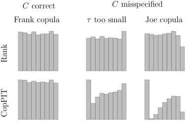
Figure 1: Multivariate rank and CopPIT histograms in the high-dimensional simulation setting described in the text.

Figure 1 shows multivariate rank and CopPIT histograms in this setting, based on a sample of $4,000$ forecast–observation pairs. The rank histograms have difficulties in detecting the deficient probabilistic forecasts due to the aforementioned discretization effect. In contrast, the CopPIT histograms for the forecasts with the misspecified copulas are non-uniform, as desired.

2.4 Directional copula calibration

The CopPIT is a natural multivariate generalization of the PIT in the univariate setting. We now discuss a further generalization that allows for directional approaches. In doing so, we refer to the probabilistic forecast for the $\mathbb{R}^{d}$-valued outcome $Y$ either by $H$ or $\mu$, with $H$ denoting a CDF and $\mu$ the associated probability measure.

Let $e_{1},\ldots,e_{d}$ be an orthonormal basis of $\mathbb{R}^{d}$ and let $\mathcal{E}$ be the closed convex cone spanned by this basis. We define the $\mathcal{E}$-CDF of the probability measure $\mu$ as

$$H^{\mathcal{E}}:\mathbb{R}^{d}\to[0,1],\qquad x\mapsto\mu(x+\mathcal{E}).$$

Any function $H^{\mathcal{E}}$ characterizes the probability measure $\mu$. The usual CDF is obtained by choosing $e_{j}=(e_{1j},\ldots,e_{dj})$ with $e_{ij}=-\mathbbm{1}(i=j)$, whereas the survival function of $\mu$ is $H^{\mathcal{E}}$ with $e_{ij}=\mathbbm{1}(i=j)$. The CopPIT depends on the particular CDF chosen, and distinct choices of $\mathcal{E}$ may reveal distinct facets of calibration or the lack thereof. In principle, one could envision a procedure in the style of a projection pursuit algorithm (Huber, 1985) that finds those $\mathcal{E}$ where the deviation of the CopPIT histogram from uniformity is the most pronounced. In the case of density forecasts a related idea was considered by Ishida (2005).

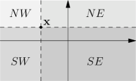
Figure 2: Illustration of quadrants for directional CopPITs

Certain choices of the cone $\mathcal{E}$ might be particularly useful. We illustrate this for $d=2$, but the idea generalizes to higher dimensions. Let SW be the convex cone spanned by $(-1,0)$ and $(0,-1)$, i.e., the south-west quadrant. Analogously we define the quadrants SE, NE, and NW, as illustrated in Figure 2. If the mariginals are probabilistically calibrated, probabilistic copula calibration with respect to $H^{\rm SW}$, which is the classical multivariate CDF, only depends on the forecast copula. This argument remain valid for $H^{\rm SE}$, $H^{\rm NE}$, and $H^{\rm NW}$, with the latter being the multivariate survival function.

Similarly, we can assess directional climatological copula calibration by plotting

$$\frac{1}{J}\sum_{j=1}^{J}\mathbbm{1}\{H^{\mathcal{E}}_{j}(y_{j})\leq w\}\quad\text{vs.}\quad\frac{1}{J}\sum_{j=1}^{J}\mathcal{K}_{H^{\mathcal{E}}_{j}}(w)$$

for $w\in[0,1]$ and suitable choices of the cone $\mathcal{E}$.

3 Simulation study

Table 1: Parameters of forecast distributions in the simulation study

Forecast	First Margin $F_{1}$	Second Margin $F_{2}$	Copula $C$
T	correct	correct	correct
	$\mu_{1}=2-B_{1}$	$\sigma_{2}^{2}=1/B_{2}$	$\tau=(B_{1}+B_{2})/2$
F	biased	underdispersed	misspecified
	$\hat{\mu}_{1}=0.8(2-B_{1})$	$\hat{\sigma}_{2}^{2}=0.8/B_{2}$	$\hat{\tau}=0.6(B_{1}+B_{2})/2$

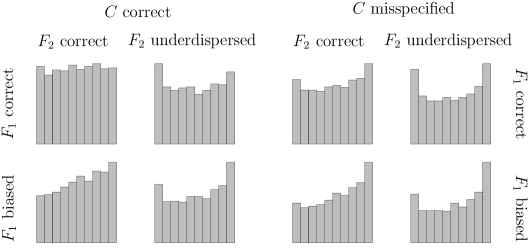
Figure 3: CopPIT histograms for the forecasters in the simulation study

We consider the following simulation setting in dimension $d=2$. Let $B_{1}$ and $B_{2}$ be independent beta variables with parameters $(\alpha_{1},\beta_{1})=(2,5)$ and $(\alpha_{2},\beta_{2})=(5,2)$, respectively. Conditional on $(B_{1},B_{2})$ the outcome vector $Y=(Y_{1},Y_{2})$ has normal margins and a Gumbel copula with Kendall’s $\tau$ equal to $(B_{1}+B_{2})/2$, as described by Nelsen (2006). The margin $Y_{1}$ has mean $\mu_{1}=2-B_{1}$ and unit variance; the margin $Y_{2}$ has mean zero and variance $\sigma_{2}^{2}=1/B_{2}$.

We assess eight probabilistic forecasters with various types of forecast deficiencies. All forecasters have access to $(B_{1},B_{2})$ and specify a Gumbel copula with Kendall’s $\tau$ equal to $\hat{\tau}$ and normal marginals, where the first margin $F_{1}$ has mean $\hat{\mu}_{1}$ and unit variance, and the second margin $F_{2}$ has mean zero and variance $\hat{\sigma}_{2}^{2}$, with details provided in Table 1. We name each forecaster with a sequence of three letters, where T stands for true and F for false. For example, the forecaster TTF specifies the first and the second marginal distributions correctly, but misspecifies the copula. The forecaster TTT is ideal with respect to the $\sigma$-algebra generated by $(B_{1},B_{2})$ in the sense defined in Section 2.1 and does not show any forecast deficiencies.

Figure 4: Univariate PIT and directional CopPIT histograms for the forecasters in the simulation study

Figure 5: Directional climatological calibration plots for the forecasters in the simulation study

Figure 3 shows CopPIT histograms for the eight forecasters based on a sample of $4,000$ forecast–observation pairs. It is interesting to observe that the standard CopPIT histogram detects misspecified marginals as well as misspecified copulas. Similar to the interpretation of univariate PIT histograms (Gneiting et al., 2007), biases yield skewed histograms, underdispersed forecasts induce a U-shape, and overdispersed forecasts an inverse U-shape.

Figure 4 shows univariate PIT histograms along with directional CopPIT histograms based on another sample of $4,000$ forecast–observation pairs. The joint consideration of the histograms can diagnose specific forecast deficiencies. As a rule of thumb, the CopPIT histograms mimic features seen in the univariate PIT histograms if the copula is well specified. In contrast, if the copula is ill specified, the CopPIT histograms show deviations from uniformity in shapes that are not necessarily reflected by the PIT histograms. Finally, Figure 5 shows directional climatological copula calibration plots. While misspecifications of the probabilistic forecasts are readily discernible, the climatological copula calibration plots appear to be more difficult to interpret diagnostically than the CopPIT histograms.

4 Case study: Probabilistic forecasts of wind vectors over the Pacific Northwest

In a recent change of paradigms, meteorologists have adopted probabilistic weather forecasting in the form of ensemble forecasts. An ensemble forecast is a collection of numerical weather prediction (NWP) model runs that are based on distinct initial conditions and/or model physics parameters (Gneiting and Raftery, 2005; Leutbecher and Palmer, 2008). Despite their undisputed success, ensemble forecasts tend to be biased and underdispersed, in the sense of the spread among the ensemble members being too small to be realistic. Therefore, methods for the statistical postprocessing of ensemble forecasts have been developed, such as the ensemble model output statistics (EMOS) approach of Gneiting et al. (2005), which generates Gaussian predictive distributions for univariate variables. In a more recent development, Schuhen et al. (2012) developed a bivariate EMOS method that generates bivariate Gaussian predictive distributions for wind vectors.

Here, we take up their work on probabilistic forecasts of surface wind vectors over the North American Pacific Northwest based on the University of Washington Mesoscale Ensemble (Eckel and Mass, 2005), which has $m=8$ members. The test data comprise calendar year 2008 with a total of 19,282 forecast–observations pairs at a prediction horizon of 48 hours. We assess and compare the raw ensemble forecast, the statistically postprocessed regional bivariate EMOS forecast developed by Schuhen et al. (2012), and an Independent EMOS forecast with the same bivariate Gaussian predictive distribution, except that the correlation coefficient is misspecified at zero.

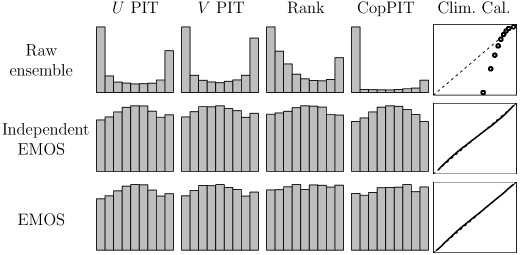
Figure 6: Univariate PIT histograms, multivariate rank histogram, CopPIT histogram and climatological CopPIT calibration plot for the raw ensemble, Independent EMOS, and EMOS forecasts of wind vectors. Following common practice, we label the wind vector components as $u$ and $v$.

Figure 6 shows univariate PIT histograms, the multivariate rank histogram, the CopPIT histogram, and the climatological copula calibration plot for the raw ensemble, Independent EMOS, and EMOS forecasts. The raw ensemble forecast shows U-shaped PIT, multivariate rank and CopPIT histograms, which attest to its underdispersion, and the climatological copula calibration plot points at severe forecast deficiencies. The univariate PIT histograms for the Independent EMOS and EMOS forecasts are identical and diagnose slight overdispersion. However, the bivariate rank and CopPIT histograms for the EMOS forecast are more uniform than for the Independent EMOS forecast, as the Independent EMOS technique fails to take dependencies between the wind vector components into account, with the CopPIT histogram providing a much clearer diagnosis than the multivariate rank histogram.

5 Discussion

In this paper, we introduced the copula probability integral transform (CopPIT), and we proposed CopPIT histograms and climatological copula calibration diagrams as diagnostic tools in the evaluation and comparison of probabilistic forecasts of multivariate quantities. These tools apply to non-parametric, semi-parametric and parametric approaches and thus can be employed to diagnose strengths and deficiencies of multivariate stochastic models in nearly any setting, be it predictive or not.

Extant methods for calibration checks for probabilistic forecasts of multivariate quantities apply either to ensemble forecasts only, such as the minimum spanning tree rank histogram and the multivariate rank histogram (Smith and Hansen, 2004; Wilks, 2004; Gneiting et al., 2008), or they apply to density forecasts only, such as the methods of Diebold et al. (1999), Ishida (2005), and González-Rivera and Yoldas (2012) that rely on the univariate PIT and the Rosenblatt transform (Rosenblatt, 1952; Rüschendorf, 2009) in one way or another. By way of contrast, CopPIT histograms and climatological copula calibration diagrams apply to all types of probabilistic forecasts, including both, ensemble forecasts and density forecasts.

In our case study, we assessed probabilistic forecasts of raw ensemble and statistically postprocessed density forecasts of bivariate wind vectors. However, our methods also apply in higher dimensions and then it may be useful to plot CopPIT histograms and climatological copula calibration diagrams for a range of subvectors of the outcome, too.

As noted, probabilistic forecasting strives to maximize the sharpness of the predictive probability distributions subject to calibration (Gneiting et al., 2007), and the methods proposed here serve to evaluate calibration only. If probabilistic forecasters are to be ranked considering both calibration and sharpness, proper scoring rules can be employed (Gneiting and Raftery, 2007; Gneiting et al., 2008), with recent theoretical advances having been made by Ehm (2011). Diks et al. (2010) and Röpnack et al. (2013) advocate the use of the logarithmic score to compare probabilistic forecasts of multivariate quantities. The event based approach of Pinson and Girard (2012) reduces a high-dimensional quantity to a binary event — essentially, the ultimate dimension reduction — and applies proper scoring rules to assess the induced probability forecasts for dichotomous events. While these techniques aim to rank probabilistic forecasters, CopPIT histograms and climatological copula calibration diagrams are diagnostic tools that strive to inform model development and spur model improvement.

References

- Barbe et al. (1996) P. Barbe, C. Genest, K. Ghoudi, and B. Rémillard. On Kendall’s process. J. Multivariate Anal., 58:197–229, 1996.
- Czado et al. (2009) C. Czado, T. Gneiting, and L. Held. Predictive model assessment for count data. Biometrics, 65:1254–1261, 2009.
- Dawid (1984) A. P. Dawid. Statistical theory: The prequential approach. J. R. Stat. Soc. A, 147:278–290, 1984.
- Diebold et al. (1998) F. X. Diebold, T. A. Gunther, and A. S. Tay. Evaluating density forecasts with applications to financial risk management. Int. Econ. Rev., 39:863–883, 1998.
- Diebold et al. (1999) F. X. Diebold, J. Hahn, and A. S. Tay. Multivariate density forecast evaluation and calibration in financial risk management: High-frequency returns on foreign exchange. Rev. Econ. Stat., 81:661–673, 1999.
- Diks et al. (2010) C. Diks, V. Panchenko, and D. van Dijk. Out-of-sample comparisons of copula specifications in multivariate density forecasts. J. Econ. Dyn. Contr., 34:1596–1609, 2010.
- Eckel and Mass (2005) F. A. Eckel and C. F. Mass. Aspects of effective mesoscale, short-range ensemble forecasting. Wea. Forecasting, 20:328–350, 2005.
- Ehm (2011) W. Ehm. Unbiased risk estimation and scoring rules. C. R. Math., 349:699–702, 2011.
- Genest et al. (2011) C. Genest, J. Nešlehová, and J. Ziegel. Inference in multivariate Archimedean copula models. Test, 20:223–256, 2011.
- Gneiting and Katzfuss (2014) T. Gneiting and M. Katzfuss. Probabilistic forecasting. Ann. Rev. Stat. Appl., in press, 2014.
- Gneiting and Raftery (2005) T. Gneiting and A. E. Raftery. Weather forecasting with ensemble methods. Science, 310:248–249, 2005.
- Gneiting and Raftery (2007) T. Gneiting and A. E. Raftery. Strictly proper scoring rules, prediction, and estimation. J. Am. Stat. Assoc., 102:359–378, 2007.
- Gneiting and Ranjan (2013) T. Gneiting and R. Ranjan. Combining predictive distributions. El. J. Stat., 7:1747–1782, 2013.
- Gneiting et al. (2005) T. Gneiting, A. E. Raftery, A. H. Westveld, and T. Goldman. Calibrated probabilistic forecasting using ensemble model output statistics and minimum CRPS estimation. Mon. Wea. Rev., 133:1098–1118, 2005.
- Gneiting et al. (2007) T. Gneiting, F. Balabdaoui, and A. E. Raftery. Probabilistic forecasts, calibration and sharpness. J. R. Stat. Soc. B, 69:243–268, 2007.
- Gneiting et al. (2008) T. Gneiting, L. I. Stanberry, E. P. Grimit, L. Held, and N. A. Johnson. Assessing probabilistic forecasts of multivariate quantities, with an application to ensemble predictions of surface winds. Test, 17:211–235, 2008.
- González-Rivera and Yoldas (2012) G. González-Rivera and E. Yoldas. Autocontour-based evaluation of multivariate predictive densities. Int. J. Forecasting, 28:328–342, 2012.
- Huber (1985) P. J. Huber. Projection pursuit. Ann. Stat., 13:435–475, 1985.
- Ishida (2005) I. Ishida. Scanning multivariate conditional densities with probability integral transforms. Center for Advanced Research in Finance, University of Tokio, Working Paper F-045, 2005.
- Leutbecher and Palmer (2008) M. Leutbecher and T. N. Palmer. Ensemble forecasting. J. Computat. Phys., 227:3515–3539, 2008.
- McNeil and Nešlehová (2009) A. J. McNeil and J. Nešlehová. Multivariate Archimedean copulas, -monotone functions and -norm symmetric distributions. Ann. Stat., 37:3059–3097, 2009.
- Nelsen (2006) R. B. Nelsen. An Introduction to Copulas. Springer, New York, 2nd edition, 2006.
- Nelsen et al. (2003) R. B. Nelsen, J. J. Quesada-Molina, J. A. Rodríguez-Lallena, and M. Úbeda Flores. Kendall distribution functions. Stat. Prob. Lett., 65:263–268, 2003.
- Pinson (2013) P. Pinson. Wind energy: Forecasting challenges for its operational management. Stat. Sci., in press, 2013.
- Pinson and Girard (2012) P. Pinson and R. Girard. Evaluating the quality of scenarios of short-term wind power generation. Appl. Energy, 96:12–20, 2012.
- Röpnack et al. (2013) A. Röpnack, A. Hense, C. Gebhardt, and D. Majewski. Bayesian model verification of NWP ensemble forecasts. Mon. Wea. Rev., 141:375–387, 2013.
- Rosenblatt (1952) M. Rosenblatt. Remarks on a multivariate transformation. Ann. Math. Stat., 23:470–472, 1952.
- Rüschendorf (2009) L. Rüschendorf. On the distributional transform, Sklar’s theorem, and the empirical copula process. J. Stat. Plann. Infer., 139:3921–3927, 2009.
- Schaake et al. (2010) J. Schaake, J. Pailleux, J. Thielen, R. Arritt, T. Hamill, L. Luo, E. Martin, D. McCollor, and F. Pappenberger. Summary of recommendations of the first workshop on Postprocessing and Downscaling Atmospheric Forecasts for Hydrologic Applications held at Météo-France, Toulouse, France, 15–18 June 2009. Atmos. Sci. Let., 11:59–63, 2010.
- Schefzik et al. (2013) R. Schefzik, T. L. Thorarinsdottir, and T. Gneiting. Uncertainty quantification in complex simulation models using ensemble copula coupling. Stat. Sci., in press, 2013.
- Schuhen et al. (2012) N. Schuhen, T. L. Thorarinsdottir, and T. Gneiting. Ensemble model output statistics for wind vectors. Mon. Wea. Rev., 140:3204–3219, 2012.
- Smith and Hansen (2004) L. A. Smith and J. A. Hansen. Extending the limits of ensemble forecast verification with the minimum spanning tree histogram. Mon. Wea. Rev., 132:1522–1528, 2004.
- Wilks (2004) D. S. Wilks. The minimum spanning tree histogram as a verification tool for multidimensional ensemble forecasts. Mon. Wea. Rev., 132:1329–1340, 2004.