Generalisation of Levine’s prediction for the distribution of freezing temperatures of droplets: A general singular model for ice nucleation

Zusammenfassung

Models without an explicit time dependence, called singular models, are widely used for fitting the distribution of temperatures at which water droplets freeze. In 1950 Levine developed the original singular model. His key assumption was that each droplet contained many nucleation sites, and that freezing occurred due to the nucleation site with the highest freezing temperature. The fact that freezing occurs due to the maximum value out of large number of nucleation temperatures, means that we can apply the results of what is called extreme-value statistics. This is the statistics of the extreme, i.e., maximum or minimum, value of a large number of random variables. Here we use the results of extreme-value statistics to show that we can generalise Levine’s model to produce the most general singular model possible. We show that when a singular model is a good approximation, the distribution of freezing temperatures should always be given by what is called the generalised extreme-value distribution. In addition, we also show that the distribution of freezing temperatures for droplets of one size, can be used to make predictions for the scaling of the median nucleation temperature with droplet size, and vice versa.

The freezing of water droplets in the Earth’s atmosphere is an important and longstanding problem (Mason, 1971; Pruppacher and Klett, 1978; Cantrell and Heymsfield, 2005; DeMott et al., 2011; Sear, 2012). We want to understand how the water droplets freeze, and be able to predict quantitatively the conditions where the droplets do and do not freeze. To do this we of course need good experimental data, but we also need models with few enough parameters that their values can be reliably obtained by fitting to experimental data. These models should make as few assumptions as possible, and we should as clear as possible as to what these assumptions are. An innovative early attempt at developing such a model was that of Levine in 1950 (Levine, 1950).

Levine assumed that water droplets freeze due to highly variable impurities in the droplets. He then introduced a simple statistical model of these impurities, and hence of the freezing behaviour (Levine, 1950). Levine’s model has no direct time dependence. Instead of an explicit rate, nucleation is assumed to occur at a particular nucleation site as soon as it is cooled to a temperature characteristic of that site. Levine’s work has inspired a literature on what are often called (Pruppacher and Klett, 1978) ‘singular’ models (Mason, 1971; Vali, 2008; Connolly et al., 2009; Niedermeier et al., 2010, 2011; Murray et al., 2011; Broadley et al., 2012; Welti et al., 2012). By definition singular models are models that lack direct time dependence. As far as I know, Levine’s is the first such singular model. He did not call his model singular, that name originates with Vali and Stansbury (1966). Singular models can be contrasted with what are called ‘stochastic’ models where there is an explicit nucleation rate for a stochastic process of nucleation, and so a direct time dependence (Pruppacher and Klett, 1978).

Levine assumed that each droplet has a large number of nucleation sites, $N$. He called these sites ‘motes’. He assumed that each mote had a different nucleation temperature, $T_{n}$, and that the droplet froze at the highest of these $N$ nucleation temperatures. This second assumption means that, within his model, the freezing temperature of a droplet, $T_{F}$, is a random number that is the maximum of a number of independent random numbers. Although Levine apparently did not realise this, this means that what he was doing was an example of what is called extreme-value statistics. This is the statistics of the extreme (maximum or minimum) of a large number of random variables. See the books of either Jondeau et al. (2007), or Castillo (1988), for an introduction to extreme-value statistics. Incidentally, back in the 1950s, Turnbull realised that Levine was effectively doing extreme-value statistics (Turnbull, 1952).

Here we use results from modern extreme-value statistics to show that the results obtained by Levine can be written in slightly simpler forms, and that they can be generalised – one of his assumptions was not necessary. The expression derived by Levine, his Eq. (2), is in fact almost (see Appendix A) the probability density function of the Gumbel distribution of extreme-value statistics. If nucleation is indeed occurring on the nucleation site with the highest nucleation temperature, then the fraction crystallised should have the form of what is called the generalised extreme value (GEV) distribution. This is true for almost all distributions of the site nucleation temperatures. The Gumbel distribution is a special case of the GEV distribution. Levine also derived a logarithmic dependence of the mode droplet freezing temperature on droplet size. We will show that this scaling is less general than the Gumbel distribution.

0.1 Motivation

Our motivation for this work is that Levine’s key assumptions are very reasonable. These assumptions are that a droplet has a large number of nucleation sites, and that nucleation occurs on the one with the highest nucleation temperature. Also, the neglect of time dependence, although an approximation, simplifies the model, meaning that the model has very few parameters. A model with few parameters is useful, as typically fitting a model with more than two or three parameters to experimental data is difficult to justify. The data may not adequately constrain the values of a larger number of parameters.

Thus Levine’s model seems a very attractive simple model that can be used to fit data directly, and can be built on to make more sophisticated models. For both these reasons it seems worthwhile to use results in modern extreme-value statistics to generalise it to produce the most general singular model possible, and to determine the minimal assumptions required for it to apply.

In this paper, we will describe Levine’s model, and then show how his key results may be derived using modern extreme-value statistics. We will then generalise Levine’s model to produce the most general possible singular model of the type that Levine introduced. In our final section, we suggest how this could be used to model experimental data.

1 Levine’s model

We are interested in the problem of what happens when a set of nominally identical liquid water droplets are cooled at some rate, until they freeze. It is observed (Levine, 1950; Langham and Mason, 1958; Mason, 1971; Pruppacher and Klett, 1978; Niedermeier et al., 2010, 2011; Murray et al., 2011; Vali, 2008; Cantrell and Heymsfield, 2005; Welti et al., 2012; Broadley et al., 2012) that the droplets do not all freeze at the same temperature; they freeze over a broad range of temperatures. We want to understand this, and make predictions about this phenomenon, using a simple model.

To do this, we define the probability $P(T_{F})$ that a randomly selected droplet has not frozen, at the time when we have cooled it down to a temperature $T_{F}$. Note that $P(T_{F})$ is a cumulative probability, the probability that a sample freezes between $T_{F}$ and $T_{F}-{\rm d}T_{F}$, is $({\rm d}P(T_{F})/{\rm d}T_{F}){\rm d}T_{F}$. In an experiment, $P(T_{F})$ can be approximated by the fraction of a large number of identically prepared droplets that are still liquid at a temperature $T_{F}$.

Levine’s model (Levine, 1950) for the freezing of liquid water droplets is simple. He made the following assumptions:

1. Each droplet contains impurities that have a total of $N$ nucleation sites.

2. Each nucleation site induces nucleation of ice rapidly at a well defined temperature $T_{n}$.

3. This temperature $T_{n}$ varies from one nucleation site to another. The sites are independent, and the values of $T_{n}$ are drawn from a probability distribution function $p_{1}(T_{n})$.

4. Only one nucleation event is required to induce crystallisation of the droplet, and so the droplet crystallises at the highest $T_{n}$ of its $N$ nucleation sites. We denote this maximum value of a set of $N$ $T_{n}$’s, by $T_{F}$.

Assumption 4 allows us to use extreme-value statistics, see Castillo (1988); Jondeau et al. (2007) for an introduction to these statistics. Here we define a singular model as being a model in which assumptions 1 to 4 are made. In particular, assumption 2 eliminates any time dependence, giving us a model with only a temperature dependence. This definition of a singular model agrees with that of Pruppacher and Klett (Pruppacher and Klett, 1978).

Levine then made a fifth assumption:

1. The distribution of nucleation temperatures at the sites, $p_{1}$, is exponential, i.e.,

   $$p_{1}(T_{n})=s\exp\left(-T_{n}/w_{e}\right)/w_{e}$$ (1)

This distribution has two parameters: $s$ (dimensionless) and $w_{e}$ (dimensions of temperature). The parameter $w_{e}$ controls how rapidly the probability of finding a site with a given $T_{n}$, decreases with increasing $T_{n}$. Note that Levine wrote this distribution in a rather different way. See Appendix A for a comparison to his work that uses notation that is closer to Levine’s.

It is worth noting that we are only interested in the highest value of $T_{n}$ of a large number of sites, and so only the large $T_{n}$ tail of the distribution $p_{1}$ is relevant here. The form of $p_{1}$ around average $T_{n}$ values is irrelevant. The maximum is never in this region. Thus we need only assume that the large $T_{n}$ tail of the distribution is exponential. The distribution around average values can be anything as these sites do not affect freezing and so have no effect in experiment. Because of this Eq. (1) is only the high-$T$ tail and so is not normalised. The parameter $s$ controls the location of this tail, i.e., the bigger $s$ is, the larger the number of sites with high nucleation temperatures.

Also, note that we expect $N$ to scale with the total surface area of the impurities present in a droplet. So if impurities are deliberately added, as for example Broadley et al. (2012) and Welti et al. (2012) did, then $N$ should be proportional to the amount added. When the impurities are those naturally present in the water, then if their concentration is constant, their amount and hence $N$ will be proportional to the droplet volume.

As an aside, we note that in the language of the statistical physics of quenched disorder, Levine’s model has quenched disorder, but no annealed disorder. The quenched disorder is the variability in the temperatures at which nucleation occurs on the sites. It is quenched disorder as it is assumed not to depend on time, but to be fixed for a given droplet. There is no annealed disorder as there is no time dependence. Annealed disorder is associated with dynamic fluctuations, which are neglected in singular models.

2 Modern derivation of Levine’s key results

If we make all 5 assumptions of section 1, we can easily derive the Gumbel distribution for the freezing temperature, $T_{F}$. The derivation of Levine’s distribution of freezing temperatures proceeds as follows. We start by obtaining the cumulative probability distribution function for a nucleation site, $P_{1}$. $P_{1}$ is the probability that the nucleation temperature at a nucleation site is lower than $T_{n}$. The cumulative probability $P_{1}$ is just a definite integral over $p_{1}$, so using the exponential $p_{1}$ of Eq. (1), we have

$$P_{1}(T_{n}) = 1-\int_{T_{n}}^{0}p_{1}(T){\rm d}T\simeq 1-\int_{T_{n}}^{\infty}p_{1}(T){\rm d}T$$ (2)

$$\simeq 1-s\exp\left(-T_{n}/w_{e}\right)$$ (3)

where we used Eq. (1) for $p_{1}$, and we extended the upper limit on integration from $0^{\circ}$C to infinity. Of course, $p_{1}$ must be zero for temperatures above $0^{\circ}$C, and so the approximate $p_{1}$ of Eq. (1) is only valid for values of $s$ and $w_{e}$ such that the exponential $p_{1}$ is negligible for $T_{n}\geq 0^{\circ}$C. We assume this to be the case here.

If a droplet contains $N$ nucleation sites then the probability that it is in the liquid phase, $P(T_{F})$, is simply the probability that all $N$ nucleation sites have crystallisation temperatures below $T_{F}$. We are assuming that even a single nucleation site will cause freezing. As these nucleation sites are independent this probability is just $P_{1}^{N}$, so,

$$P(T_{F},N) = P_{1}^{N}=\left[1-s\exp\left(-T_{F}/w_{e}\right)\right]^{N}$$ (4)

$$\simeq \exp\left[-Ns\exp\left(-T_{F}/w_{e}\right)\right]$$ (5)

Here we used the fact that when $N$ is large, we are interested in the range when $s\exp\left(-T/w_{e}\right)\ll 1$, and so we can use the result $(1+x)^{n}\simeq\exp(nx)$, which is valid for small $x$ and large $n$.

We can rewrite $P$ as

$$P(T_{F},N)=\exp\left[-\exp\left(-\left[T_{F}-w_{e}\ln(Ns)\right]/w_{e}\right)\right]$$ (6)

This is the cumulative distribution function for the Gumbel extreme-value distribution (Castillo, 1988; Nicodemi, 2009; Jondeau et al., 2007). The Gumbel distribution is a special case of the GEV distribution. This Gumbel $P$ is plotted in Fig. 1(A).

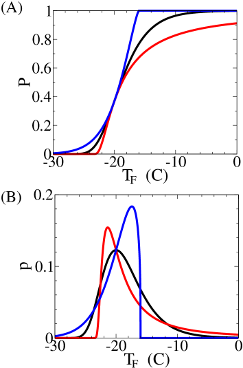
Abbildung 1: Plots of: (A) the cumulative distribution function $P(T_{F})$, and (B) the probability density function $p(T_{F})$. $T_{F}$ is the temperature a droplet freezes. In both plots the black, red and blue curves are the Gumbel, Fréchet and Weibull distribution functions, respectively. For the Fréchet distributions $\xi=0.75$, while for the Weibull distributions $\xi=-0.75$. For all curves, the location $\mu=-20^{\circ}$C, and the width $w=3^{\circ}$C. For the $P$’s we use Eq. (9). Note that for the Gumbel distribution, $\mu$ and $w$ are related to $s$, $N$ and $w_{e}$, by $\mu=w_{e}\ln(sN)$ and $w=w_{e}$.

For an exponential $p_{1}$, the width of the Gumbel distribution of crystallisation temperatures is the same as the width $w_{e}$ for a single nucleation site. The median crystallisation temperature, $T_{MED}$, is obtained by noting that, by the definition of the median, $P(T_{MED})=1/2$. Then we have that the median freezing temperature is

$$T_{MED}(N)=w_{e}\ln s-w_{e}\ln(\ln 2)+w_{e}\ln(N)$$ (7)

The scaling of the average freezing temperature with the number of nucleation sites is logarithmic, as Levine found in his Eq. (10). The variation of $T_{MED}$ with $N$ is shown in Fig. 2(A). Finally, the probability density function for nucleation to occur at a temperature $T_{F}$, $p(T_{F})$, is

$$p(T_{F}) = \frac{{\rm d}P(T_{F})}{{\rm d}T_{F}}$$ (8)

$$= P(T_{F})\exp\left[-\left(T_{F}-w_{e}\ln(Ns)\right)/w_{e}\right]/w_{e}$$

This is almost equal to Levine’s Eq. (2) for $p(T)$. It is not quite equal as Levine made a small approximation. We compare our expressions with Levine in detail in Appendix A. The Gumbel $p$ is plotted in Fig. 1(B). Note that the Gumbel distribution has a characteristically fatter tail on the high-temperature side than on the low-temperature side of its maximum. This is often seen in experimental data for the freezing of water droplets, for example in Fig. 52 of Langham and Mason (1958).

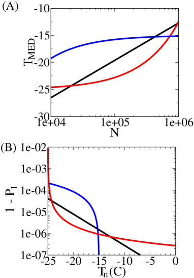
Abbildung 2: (A) Plot of the scaling of the median freezing temperature, $T_{MED}$, with the number of nucleation sites, $N$. The black curve is the $\ln N$ scaling that is consistent with the Gumbel distribution. It is a plot of the $T_{MED}$ of Eq. (7), with parameters $s=10^{-8}$ and $w_{e}=3^{\circ}$C. The red curve is the $N^{3/4}$ scaling that is consistent with the Fréchet distribution with $\xi=0.75$. It is a plot of the $T_{MED}$ of Eq. (16), with parameters $b=2\times 10^{-5}$ and $T_{L}=-25^{\circ}$C. The blue curve is the $N^{-3/4}$ scaling that is consistent with the Weibull distribution with $\xi=-0.75$. It is a plot of the $T_{MED}$ of Eq. (17), with parameters $c=10^{-5}$ and $T_{U}=-15^{\circ}$C. (B) Plot of cumulative distribution functions for the nucleation temperatures, $T_{n}$, at the nucleation sites. We clarity, we plot $1-P_{1}(T_{n})$, i.e., the probability that a nucleation site has a nucleation temperature above $T_{n}$. This tends to 0 not 1 at high $T$. The black, red and blue curves are $1-P_{1}$’s that yield Gumbel, Fréchet, and Weibull distributions, respectively. Values of the parameters are the same as in (A).

3 Predictions of modern extreme value statistics

The Gumbel distribution that Levine derived is just one of the three types or classes of extreme-value distributions, that together make up the GEV (Nicodemi, 2009; Jondeau et al., 2007; Castillo, 1988). The other two are the Weibull and Fréchet distributions. In brief, modern extreme value theory allows us to show that for any singular model, $P(T_{F})$ should be given by the GEV. The requirements that must be satisfied are only that assumptions 1 to 4 must hold, and that $p_{1}$ should be a simple continuous function of $T$ in the temperature range of interest.

In this section we use modern extreme-value statistics to generalise Levine’s findings, in order to obtain the more general GEV form of $P(T_{F})$. We also derive the scaling of the average freezing temperature, $T_{MED}$, with $N$ for the Weibull and Fréchet distributions, and compare the results with experimental data. We will briefly consider how good our assumption that $N$ is the same in droplets of the same volume. Also, as our model is in the singular limit, we outline a criterion for the singular limit to be a good approximation.

3.1 The generalised extreme value distribution

Once assumptions 1 to 4 are made, the freezing temperature $T_{F}$ is the maximum of a large number of independent identically distributed random variables. Then it can be shown that the cumulative distribution function for $P(T_{F})$ is given by the GEV. This is true under only weak conditions on $p_{1}$ (Nicodemi, 2009; Castillo, 1988; Jondeau et al., 2007), The GEV is conventionally written as (Castillo, 1988; Nicodemi, 2009; Jondeau et al., 2007)

$$P(T_{F})=\left\{\begin{array}[]{lc}\exp\left[-\exp\left(-\left(T_{F}-\mu\right)/w\right)\right]&\xi=0\\ \exp\left[-\left(1+\xi\left(T_{F}-\mu\right)/w\right)^{-1/\xi}\right]&\xi\neq 0\end{array}\right.$$ (9)

This is a three-parameter cumulative probability distribution function. Assumption 5 is not required to derive it. The parameters are a width parameter $w$, a location parameter $\mu$, and an exponent $\xi$. The value of the parameter $\xi$ controls the class of the GEV. With $\xi=0$, the GEV is the Gumbel distribution, while for $\xi>0$, the GEV is the Fréchet distribution, and for $\xi<0$, it is the Weibull distribution. Examples of all three distributions are plotted in Fig. 1.

Equation (9) generalises the Gumbel distribution, Eq. (6), that Levine derived. Whereas the Gumbel distribution is produced by exponentially decaying (in the sense of decaying faster than any power law) $p_{1}$’s, almost any continuous simple $p_{1}$ will lead to the GEV. This includes $p_{1}$’s that decay as power laws. Power law $p_{1}$’s lead to the Fréchet limit of the GEV, and $p_{1}$’s with upper limits lead to the Weibull distribution.

The form of the distribution of nucleation temperatures, $p_{1}$, also determines the scaling of the median freezing temperature with $N$. We have already seen that for an exponential $p_{1}$, this scaling is $\ln N$, Eq. (7). This $p_{1}$ also leads to a Gumbel $P(T_{F})$, but other $p_{1}$’s lead to the same Gumbel form for $P$ but have different scaling of $T_{MED}$ with $N$. For example a Gaussian $p_{1}$ leads to a $(\ln N)^{1/2}$ scaling (Castillo, 1988).

What this means is that if, for example, data is well fit by a Gumbel $P$, i.e., $\xi\simeq 0$, then we cannot argue that $T_{MED}$ scales as $\ln N$ – although it should be noted that $\ln N$ and $(\ln N)^{1/2}$ scaling are relatively similar so if it is a Gumbel then we do have a rough idea of the scaling of $T_{MED}$. However, if data is clearly best fit by a $\ln N$ scaling of $T_{MED}$, then this is good evidence that $p_{1}$ is indeed an exponential function of $T_{n}$, in the temperature range of interest. It is stronger evidence for an exponential $p_{1}$, than the Gumbel distribution providing a good fit to $P$.

Fitting the GEV could be done following the same methods used to fit the GEV to data in other fields. The book of Castillo (1988) on extreme value statistics discusses general fitting approaches. It is worth noting that he does not recommend the standard unweighted least-squares fitting procedure as that gives a low weight to errors in the tail of $P(T_{F})$. See Castillo (1988) for suggested weighting functions to be minimised in fitting. Castillo (1988) also discusses the fact that plots of $\ln[\ln(1/P(T_{F}))]$ as a function of $T_{F}$, show a characteristic curvature that depends on $\xi$. This can be used to differentiate between Gumbel, Fréchet and Weibull distributions. Such a plot should be a straight line if the data follows the Gumbel distribution, while it will curve down for Weibull-distributed data, and up for Fréchet-distributed data.

Jondeau et al. (2007) discuss a related method, which uses what are called Quantile-Quantile or Q-Q plots. Here the temperature at which the GEV function for $P$ is a particular value, is plotted as a function of the temperature in the data which gives the same value for $P$. When this is done, then if the data is indeed well approximated by the GEV, and the correct value of $\xi$ is chosen, then the Q-Q plot will be a straight line (arbitrary values of $\mu$ and $w$ can be used as they just change the slope and intercept of the plot). See Jondeau et al. (2007) for details. They also consider the application of maximum likelihood methods to obtaining the most reliable estimates of $\xi$, $\mu$ and $w$.

In the next section, we outline how both the Fréchet and Weibull distributions can be derived from their respective $P_{1}$’s. This also allows us to also determine how the median freezing temperature, $T_{MED}$, scales with $N$.

3.2 Brief derivation of the Fréchet and Weibull distributions

In this section we briefly show how the Fréchet and Weibull distributions can be derived from the $P_{1}$’s of the nucleation sites, where as before $P_{1}(T_{n})$ is the probability that the nucleation temperature at a site is below $T_{n}$. As the $N$ nucleation sites are independent, we always have that the probability that a droplet has not frozen at a temperature $T_{F}$ is

$$P(T_{F})=P_{1}^{N}(T_{n})$$ (10)

which as we are in $N\gg 1$, and $1-P_{1}\ll 1$ limit can be written as

$$P(T_{F}) = \left[1-[1-P_{1}(T_{F})]\right]^{N}(T_{n})$$ (11)

$$\simeq \exp\left[-N[1-P_{1}(T_{F})]\right]$$

Armed with this relation, we start with the Fréchet distribution. The Fréchet distribution results from a power-law cumulative distribution, $P_{1}$, for nucleation temperatures $T_{n}$,

$$P_{1}(T_{n})=1-\frac{b}{(T_{n}-T_{L})^{1/\xi}}\leavevmode\nobreak\ \leavevmode\nobreak\ \leavevmode\nobreak\ \leavevmode\nobreak\ \leavevmode\nobreak\ \leavevmode\nobreak\ \xi>0$$ (12)

Note that this is a power-law decay with a lower cutoff, $T_{L}$. The parameter $b$ (like $s$) controls the size of the tail. This expression holds for the large $T_{n}$ tail, where $P_{1}$ is close to 1. Note that here, we have the restriction that $\xi>0$, so this is a power-law decay of $p_{1}$ with $T_{n}$. In Fig. 2(B), we have plotted an example $P_{1}$. We plot $1-P_{1}$ not $P_{1}$ itself, as $1-P_{1}$ decays to 0, and this is a little clearer to see than a decay to 1. The cumulative probability $1-P_{1}(T_{n})$ is the probability that a nucleation site has a nucleation temperature above $T_{n}$. Now, using the $P_{1}$ of Eq. (12) in Eq. (11), we have the Fréchet distribution

$$P(T_{F})\simeq\exp\left[-\frac{Nb}{(T_{F}-T_{L})^{1/\xi}}\right]$$ (13)

Note that $N$ and $b$ always appear as their product, $Nb$. Therefore, the freezing behaviour does not depend on $N$ and $b$ separately, only on their product.

We now consider the Weibull distribution. The Weibull distribution results from a cumulative distribution, $P_{1}$, with an upper cut off

$$P_{1}(T_{n})=\left\{\begin{array}[]{cc}1-c(T_{U}-T_{n})^{-1/\xi}&T_{n}\leq T_{U}\\ 1&T_{n}>T_{U}\end{array}\right.\leavevmode\nobreak\ \leavevmode\nobreak\ \leavevmode\nobreak\ \leavevmode\nobreak\ \leavevmode\nobreak\ \leavevmode\nobreak\ \xi<0$$ (14)

where $T_{U}$ is the upper cutoff, and $c$ is a parameter that (like $s$ and $b$) controls the size of the tail. This expression holds for the large $T$ tail, where $P_{1}$ is close to 1. Note that here, we have the restriction that $\xi<0$, so $1-P_{1}$ is a positive-exponent power-law function of $T_{n}$. An example $1-P_{1}$ is plotted in Fig. 2(B).

In the singular limit, a hard upper cutoff, $T_{U}$, to the distribution of nucleation temperatures, is possible. In experiment, there will presumably be a limit to how well defined this cutoff temperature can be. In practice, the Weibull model should be a good model for experimental data when the inevitable uncertainty in $T_{U}$, call it $\delta T_{U}$, is much smaller than the range of temperatures over which nucleation occurs. This range of temperatures could be measured by the standard deviation of the observed nucleation temperatures, $\sigma_{F}$. So when $\delta T_{U}\ll\sigma_{F}$, and the Weibull model fits the data well, the Weibull model should be useful.

Returning to the $P_{1}$ of Eq. (14). If we put this in Eq. (11), we have the Weibull distribution

$$P(T_{F})\simeq\exp\left[-Nc(T_{U}-T_{F})^{-1/\xi}\right]$$ (15)

Having derived the Gumbel, Fréchet, and Weibull distributions, we can compare them. Example plots are shown in Fig. 1. The differences between the three distributions is particularly clear in the plots of their probability densities in Fig. 1(B). The Fréchet distribution has a much fatter high-temperature tail than the Gumbel, and a low-temperature cutoff. So, if the GEV is fit to data with such a sharp lower-temperature cutoff and/or fat tail, the best fit may be with a $\xi>0$, implying that a Fréchet distribution is a better model than a Gumbel. The fatter tail of the Fréchet comes from a power-law tail in $p_{1}$, i.e., from a fatter tail in the distribution in the nucleation temperatures at the individual sites. By contrast, the Weibull distribution has a high-temperature cutoff, which implies a high-temperature cutoff in $p_{1}$. For data with a sharp upper cutoff to nucleation, the Weibull model may be best.

3.3 Scaling of $T_{MED}$ with droplet volume and surface area of added impurity

An exponential $P_{1}$ led to a Gumbel distribution, and $\ln N$ scaling of the median freezing temperature with $N$. Here we derive the corresponding scalings with system size for power-law $P_{1}$’s, and $P_{1}$’s with upper limits.

Power-law $P_{1}$’s lead to the Fréchet $P(T_{F})$ of Eq. (13). The median freezing temperature, $T_{MED}$, is the temperature at which $P=1/2$, and so here we have

$$T_{MED}=T_{L}+\left(\frac{b}{\ln 2}\right)^{\xi}N^{\xi}$$ (16)

The median freezing temperature is a power-law function of the number of nucleation sites, $N$. This is illustrated in Fig. 2(A).

$P_{1}$’s with an upper cutoff lead to the Weibull $P(T_{F})$ of Eq. (15). The median freezing temperature, $T_{MED}$, is again the temperature at which $P=1/2$, and so here we have that

$$T_{MED}=T_{U}-\left(\frac{c}{\ln 2}\right)^{\xi}N^{\xi}$$ (17)

The median freezing temperature approaches the upper limit, $T_{U}$, of the nucleation temperatures, as $N\to\infty$. This is shown in Fig. 2(A). This hard cutoff to the nucleation temperatures will presumably be only an approximation to the truth. However, Eq. (17) should be a good approximation when the inevitable uncertainty in $T_{U}$ is small in comparison with the change in $T_{MED}$ with $N$.

Having determined the scaling of $T_{MED}$ with $N$ for all three classes of the GEV, we can compare these predictions with experimental findings. There have been a number of studies of the average freezing temperature of droplets. Both the droplet volume, and the surface area of added impurity have been varied. A plot of the average nucleation temperatures obtained in early work is shown in Mason’s book (Mason, 1971), in Fig. 4.2. On the log-linear scale, some data is linear, which is consistent with an exponential-tailed $p_{1}$, whereas other data sets appear to be plateauing at large droplets, suggesting an upper cutoff to $p_{1}$.

In more recent work, both Broadley et al. (2012), and Welti et al. (2012) have studied average nucleation temperatures as a function of the surface area of added clay particles. The clay is illite for Broadley et al., and kaolinite for Welti et al.. We expect the number of nucleation sites, $N$, to scale with the surface area of added clay. Broadley et al. (2012)’s data seem to be plateauing at large amounts of added illite clay. This is in their Fig. 4. Welti et al. (2012) observe a logarithmic scaling of the median nucleation temperature with clay surface area. Thus, the data on the scaling of the freezing temperature with system size, suggests that ice nucleation is occurring on sites with either an exponentially decaying $p_{1}$, or a $p_{1}$ with an upper cutoff.

3.4 Validity of the asssumption that $N$ is the same for all droplets

If in experiment, the variable is the amount of an impurity that is added, then it seems a safe assumption that $N\propto$ surface area of added impurity, and that two droplets with the same amount of added impurity have the same number of nucleation sites, $N$. This just relies on there being a density of nucleation sites on the surface, that is approximately constant.

However, if the variable is droplet volume $V$, then we are relying on $N\propto V$ and each droplet having the same number of nucleation sites, $N$. If the nucleation sites are distributed over a large number, $n$, of impurity particles then the Central Limit Theorem of statistics tells us that the variation in $N$ from one droplet to another will be of order $N/n^{1/2}$. Thus for $n\gg 1$ this will be small and our assumption of constant $N$ will be only a small approximation. However, if $n$ is small, i.e., each droplet has only a few impurity particles, then even though each may have many nucleation sites, there will be large fluctuations in $N$ from one droplet to another of the same volume. These fluctuations could potentially cause deviations from the (GEV) distribution, due to some droplets having many more nucleation sites than others.

3.5 Validity of the singular limit

The assumption that nucleation occurs at a site at a precisely determined temperature, $T_{n}$, is presumably only an approximation to the truth. If ice nucleation in a droplet occurs at a temperature-dependent stochastic rate, $R(T)$, then nucleation will occur over a temperature range of some width $\Delta T_{S}$. This width is expected to scale as

$$\Delta T_{S}=\left(\frac{1}{R}\frac{\partial R}{\partial T}\right)_{R=R_{COOL}}^{-1}$$ (18)

The expression in brackets is the ratio of the temperature derivative of the rate, to the rate itself. One over this ratio is an approximation to the change in temperature needed to double the nucleation rate. This ratio is evaluated at a temperature such that the nucleation rate, $R$, equals the cooling rate, $R_{COOL}$, in experiment. Note that it is non-negligible assumption that a well-defined nucleation rate exists in these systems (Sear, 2013).

In words, the expected spread in nucleation temperatures, $\Delta T_{S}$ due to a temperature-dependent nucleation rate, is approximately equal to the temperature change needed to double the nucleation rate. This temperature change is evaluated when the nucleation rate equals the cooling rate.

The singular limit is then the limit $w\gg\Delta T_{S}$. When the width in the spread of freezing temperatures due to the spread in characteristic nucleation temperatures, $T_{n}$, is much larger than the spread due to the stochastic nucleation rate, then singular models can be a good approximation to experimental data. But when the spread due to the stochastic nature of the nucleation, $\Delta T_{S}$ is comparable to that due to the variability in nucleation temperatures, then singular models will be poor approximations.

Singular models have been and are being used to fit experimental data (Mason, 1971; Pruppacher and Klett, 1978; Vali, 2008; Niedermeier et al., 2010; Broadley et al., 2012). The fact that they work so well suggests that in many situations an explicit time dependence does not need to be considered. Here we have shown within a general singular model, the distribution of freezing temperatures should be given by the GEV. This follows if, as Pruppacher and Klett (1978) do, a singular model is defined as being assumptions 1 to 4, and $p_{1}$ is a simple function of temperature.

There is a caveat to this statement. This is that for $P(T_{F})$ to be given by the GEV, it is necessary that over the temperature range of interest, $P_{1}(T_{n})$ should be given by a single continuous function, such as a power law or exponential. This may not be the case if there is more than one type of nucleation site (perhaps due to multiple particle species) which all make significant contributions to $P_{1}$ but have different dependences on temperature. Thus it may be that even in the singular limit, $P(T_{F})$ deviates from the GEV in the presence of nucleation on a complex mixture of impurities. Then there is no general theory. Here calculating $P(T_{F})$ can only be done if the distribution of nucleation temperatures at the sites is known $p_{1}$. This will presumably be difficult even for simple impurities. However, if we have experimental data for $P(T_{F})$, then Eq. (11) tells us that if we plot $\ln P(T_{F})$ as a function of $T_{F}$, then we should be plotting $-N[1-P_{1}]$. Then what we are plotting is directly proportional to the cumulative probability of finding a nucleation site with a nucleation temperature above $T_{F}$. This may aid in interpreting data for $P(T_{F})$.

Microscopic models of nucleation, for example those based on classical nucleation theory, are also used to fit and understand experimental results (Cantrell and Heymsfield, 2005; Niedermeier et al., 2011). They can provide insight into droplet freezing data that a purely statistical model such as an extreme-value-statistics model cannot provide. However, in the singular limit ($\Delta T_{S}\ll w$) almost any microscopic model will give the GEV. Thus in this limit any two microscopic models with similar $P_{1}$ will be essentially equivalent.

Finally, in practice if data deviates from the GEV, it may be difficult to assess why, as there could be several reasons for the deviations. These include: 1) effects of a stochastic temperature-dependent rate, of the type that classical nucleation theory predicts; 2) a complex $p_{1}$ due to a mixture of surfaces, all making significant contributions to nucleation; 3) non-classical-nucleation-theory time-dependent processes, for example, irreversible chemical processes at surfaces that change the ability of a surface to promote ice nucleation; (4) each droplet contains only a handful of impurity particles with the nucleation sites, and so some droplets have many more nucleation sites ($N$) than others. Distinguishing between the four may be difficult, although varying the cooling rate may be one way to eliminate at least some of them.

3.6 Suggestions for future work

It may be worthwhile to do what is standard practice in other fields where extreme-value statistics are used, and to fit the GEV distribution to the data. Here the data is the fraction of droplets that have frozen, as a function of temperature. If the fit is good, then the data would be consistent with an extreme-value model, and if the fitted $\xi$ is close to zero, it would suggest that the high $T$ tail of the nucleation temperatures of individual sites is indeed exponential or similar, i.e., decays faster than a power law (Nicodemi, 2009). However, a value of $\xi>0$ suggests a power law decay for $p_{1}$, while $\xi<0$ suggests an upper limit beyond which $p_{1}=0$. In other words, the value of $\xi$ gives information on the form of $p_{1}$.

Another point of view, is that assumptions 1 to 4 (only), lead to the GEV, and so the GEV can be used to decouple assumptions 1 to 4, from assumption 5. Assumptions 1 to 4 are presumably only approximately true. In particular, assumption 2 that a site induces nucleation at a temperature independent of cooling rate is presumably only approximate. To rigorously test for violations of this assumption, which is at the heart of singular models, we would like to avoid assumption 5, and so should tests for deviations from the GEV, not from the Gumbel distribution.

A final point to note is that the high-$T$ tail in $p_{1}$, not only determines $P(t)$, but also determines the scaling of the median nucleation temperature with $N$. In general, the fatter the tail in $p_{1}$, the faster the median nucleation temperature varies with $N$. This is illustrated in Fig. 2(A). So if a fit to a $P(t)$ produces a $\xi>0$ then the volume dependence should be faster than logarithmic, the median freezing temperature should scale as $N^{\xi}$. A best fit value of $\xi<0$ suggests a Weibull distribution, which has an upper cutoff and hence an upper limit to the median nucleation temperature as droplet volume is increased.

Anhang A Comparison with Levine’s expression

Levine’s approximation for the probability that nucleation has not occurred at a temperature $T$ is the first factor in his Eq. (2). We write this as

$$P(T)=\left(1-\frac{1}{\mu}\right)^{ar^{-T}}\leavevmode\nobreak\ \leavevmode\nobreak\ \leavevmode\nobreak\ \leavevmode\nobreak\ r>1$$ (19)

where we have taken the dominant term in his exponent, $ar^{-T}$, and changed what is a $+T$ in Levine’s expression to a $-T$. Levine uses the absolute value of $T$ in Celsius, so his $T$ is our $-T$. In this expression $\mu=V_{R}/\Delta V$, where $\Delta V$ is the volume of a droplet, and $V_{R}$ is a large reservoir volume, $\gg\Delta V$. The droplet volume $\Delta V$ is proportional to our $N$. The parameter $a$ is is analogous to our $s$ parameter. The $r$ parameter controls the width of Levine’s distribution, so it is analogous to our $w_{e}$.

If we note that both $\mu$ and $ar^{-T}\gg 1$, we can rewrite Eq. (19) as an exponential

$$P(T,\mu) = \exp\left[-\frac{ar^{-T}}{\mu}\right]$$ (20)

$$= \exp\left[-\exp\left[-T\ln r+\ln\left(\frac{a}{\mu}\right)\right]\right]$$

If we compare this equation with Eq. (6), we see that they are the same if $\ln r=1/w_{e}$, and $a/\mu=Ns$. Also, from this equation it is easy to show that the median nucleation temperature, $T_{MED}$, scales as $\ln(1/\mu)\propto\ln\Delta V$.

Levine’s Eq. (2) is actually his approximation for the probability density, $p$, that nucleation has occurred at a temperature $T$ not the cumulative probability that it has not occurred down to a temperature $T$. This $p={\rm d}P/{\rm d}T$. The expression in Levine’s Eq. 2 is not quite the $T$ derivative of Eq. (20), as Levine treats $T$ as a discrete variable when it is a continuous variable. Thus the expression in his Eq. (2) is, for this reason, approximate. But this should not obscure the fact that Levine was the first to realise that the extremes of the distribution of nucleation sites determine the nucleation behaviour, and that the use of what is essentially extreme-value statistics can be used to model freezing behaviour.