Long-lived PeV–EeV Neutrinos from GRB Blastwave

Abstract

Long duration gamma-ray bursts are powerful sources that can accelerate particles to ultra-high energies. Acceleration of protons in the forward shock of the highly relativistic GRB blastwave allows PeV–EeV neutrino production by photopion interactions of ultra-high energy protons with X-ray to optical photons of the GRB afterglow emission. Four different blastwave evolution scenarios are considered: adiabatic and fully radiative blastwaves in a constant density circumburst medium and in a wind environment with the particle density in the wind decreasing inversley proportional to the square of the radius from the center of the burst. The duration of the neutrino flux depends on the evolution of the blastwave, and can last up to a day in the case of an adibatic blastwave in a constant density medium. Neutrino fluxes from the three other blastwave evolution scenarios are also calculated. Diffuse neutrino fluxes calculated using the observed rate of long-duration GRBs are consistent with the recent IceCube upper limit on the prompt GRB neutrino flux below PeV. The diffuse neutrino flux needed to explain the two neutrino events at PeV energies recently detected by IceCube can partially come from the presented GRB blastwave diffuse fluxes. Future observations by IceCube and upcoming huge radio Askaryan experiments will be able to probe the flux models presented here or constrain the GRB blastwave properties.

I Introduction

The current paradigm of a long-duration (typical duration $\sim 10$ s) Gamma-Ray Burst (GRB) is based on core-collapse of a massive ($\gtrsim 30M_{\odot}$) progenitor star MacFadyen:1998vz ; Woosley:2005gy to a blackhole or highly magnetized neutron star (central engine) with subsequent emission of a short-lived and highly relativistic jetted ejecta Meszaros:1993cc , with a bulk Lorentz factor $\Gamma\gtrsim 100$–$1000$. Highly variable, on time scales as short as $\Delta t\sim 10^{-3}$ s, prompt $\gamma$-ray emission in the keV–MeV range is thought to originate from the ejecta matreial in the jet itself Rees:1994nw , although the exact emission mechanism is unknown. Synchrotron radiation by electrons that are accelerated in the shocks between outflowing materials inside the GRB jet (internal shocks) and/or thermal radiation from the jet photosphere are plausible mechanisms to produce the observed keV–MeV $\gamma$ rays (see, e.g., Refs. Piran:2004ba ; Zhang:2003uk for reviews). Protons co-accelerated with electrons in the internal shocks to Ultra High Energies (UHE, $\gtrsim 10^{18}$ eV) have been proposed Waxman:1995vg as UHE Cosmic Rays (UHECRs), once escaped from the GRB jet and observed on the Earth.

Acceleration of UHECRs in the internal shocks leads to TeV–PeV $\nu$ production from interactions of CR protons with the ambient keV–MeV photons via $p\gamma$ interactions Waxman:1997ti . The radii from the central engine at which the internal shocks take place, however, depend crucially on $\Gamma$. Optimistic calculations with $\Gamma\sim 100$ and $\Delta t\sim 10^{-3}$ s result in a radius small enough for the $p\gamma$ interaction opacity to reach $\sim 1$, thus efficient production of $\nu$’s in the TeV–PeV range. No such $\nu$’s, correlated with GRBs, have been detected by the IceCube Neutrino Observatory Abbasi:2012zw or by the ANTARES neutrino telescope Adrian-Martinez:2013sga from stacking analysis of GRBs which took place during their respective operations in the last few years. These results severely constrain the most optimisitc internal-shock $\nu$ flux models (see, however, Refs. Dermer:2003zv ; Murase:2005hy ; Hummer:2011ms ). One possibility, barring a scenario where GRBs are inefficient accelerators of UHECRs, is that GRBs have larger $\Gamma$ than used for $p\gamma$ opacity calculation. Recent modeling of GeV $\gamma$-ray data from the Fermi Gamma Ray Space Telescope also reveals that $\Gamma\gg 100$ at least for a large fraction of the GRBs (see, e.g., Ref. Gehrels:2013xd ) detected by its high-energy ($\gtrsim 20$ MeV–300 GeV) instrument, the Large Area Telescope (LAT) Atwood:2009ez .

The GRB jet drives a blastwave ahead of the ejecta and slows down by accumulating particles from the ambient medium. After a time $t=t_{dec}$ when the kinetic energies of the blastwave and the ejecta are roughly equal, the blastwave decelerates in a self-similar fashion Blandford:1976uq . Synchrotron radiation by electrons in the external forward shock of such a decelerating blastwave has successfully described multiwavelength observation — from X rays to radio — of GRB afterglows Meszaros:1996sv ; Sari:1997qe . Detection of sustained GeV emission by Fermi-LAT, long after the GRB prompt emission phase is over and with smoothly decaying flux characteristcs as observed in X-ray to radio afterglows, from a number of GRBs provide strong evidence DePasquale:2009bg ; Fermi+110731A that long-lived GeV emission is also part of the afterglow Kumar:2009vx ; Ghisellini+10 . This requires acceleration of electrons to the maximum allowable limit from synchrotron cooling and often exceeding it Piran:2010ew ; Atwood:2013dra . A combined electron-proton synchrotron radiation scenario, during the coasting phase of the GRB fireball Razzaque:2009rt and during the deceleration phase of the blast wave Razzaque:2010ku , may alleviate this problem.

Indeed protons co-accelerated with the electrons in the GRB blastwave have been suggested to produce UHECRs Vietri:1995hs . These protons, if interacting with electron-synchrotron photons in the blastwave, should also produce $\nu$’s via $p\gamma$ interactions. In this work, using analytic and numerical methods, we calculate fluxes of these $\nu$’s based on different blastwave evolution scenarios. We assume $\Gamma\gg 100$ and rapid slow down of the GRB blastwave on a time scale $\sim 10$ s, as would be required to explain GeV $\gamma$-ray emission from the external forward shock in the blastwave. Note that our $\nu$ flux model is different from those in Refs. Waxman:1999ai ; Dai+01 who calculated fluxes from the short-lived external reverse shock that propagates into the ejecta material which may produce optical emission at an earlier stage of the GRB evolution (see, however, Ref. Murase:2007yt for a long-lived $\nu$ flux emission model from the reverse shock in connection with shallow-decay X-ray light curve after the prompt $\gamma$-ray emission Nousek:2005fm ; Zhang:2005fa ). The $\nu$ fluxes that we calculate last for a longer time, albeit with progressively lower intensity in time. Earlier work on forward-shock neutrino emission focused on adiabatic blastwave model in constant density medium Dermer:2000yd ; Li:2002dw . Here we carry out comprehensive study of four different blastwave evolution models.

The organization of this paper is as follows. In Sec. II we set up our physical model of the GRB blastwave and target photon field for $p\gamma$ interactions. We calculate $\nu$ fluxes in Sec. III from a CR acceleration scenario and briefly discuss $\nu$ detection prospects in Sec IV. We discuss our results and draw conclusions in Sec. V. A number of essential formulas are provided in Appendix A in order to calculate the synchrotron photon spectra in the GRB blastwave which are targets for $p\gamma$ interactions. We also give analytic expressions to calculate $p\gamma$ opacities and CR parameters in Appendix  B. Some scaling formulas for pion and muon decays are given in Appendix C.

II $p\gamma$ interaction in GRB blastwave

We consider photopion production mechanism and associated chain decay of charged pion and muon ($\pi^{+}\to\mu^{+}+\nu_{\mu}\to e^{+}+\nu_{e}+{\bar{\nu}}_{\mu}+\nu_{\mu}$ and charge conjugate reactions for $\pi^{-}$) for UHE $\nu$ flux calculation from a GRB blastwave. We assume that UHECRs are accelerated in the forward shock that propagates into the blastwave and interact with synchrotron photons from electrons which are accelerated in the same shock. The observed synchrotron spectrum which would constitute the target photons for $p\gamma$ interactions, however, depends on the properties of the GRB blastwave and the surrounding environment. We discuss this briefly here and refer interested readers to Refs. Sari:1997qe ; Chevalier+00 ; Granot:2001ge ; Panaitescu:2001fv ; Ghisellini+10 for further details.

II.1 Blastwave models and synchrotron flux

Given an isotropic-equivalent kinetic energy $E_{k}=10^{55}E_{55}$ erg and an inital bulk Lorentz factor $\Gamma_{0}=10^{2.5}\Gamma_{2.5}$, the GRB ejecta (fireball) in the Inter-Steller Medium (ISM) of uniform density $n(R)=n_{0}$ cm^-3; where $R$ is the distance from the center of the explosion, decelerates on a time scale

$$t_{dec,i} = \left[\frac{3E_{k}(1+z)^{3}}{64\pi nm_{p}c^{5}\Gamma_{0}^{8}}\right]^{1/3}$$ (1)

$$= 33.3\,(1+z)n_{0}^{-1/3}\Gamma_{2.5}^{-8/3}E_{55}^{1/3}~{}{\rm s}.$$

In case of a wind-type medium with a density profile $n(R)=AR^{-2}$, the deceleration time scale is

$$t_{dec,w} = \frac{E_{k}(1+z)}{16\pi Am_{p}c^{3}\Gamma_{0}^{4}}$$ (2)

$$= 1.5\,(1+z)A_{\star}^{-1}\Gamma_{2.5}^{-4}E_{55}~{}{\rm s},$$

where $A={\dot{M}}_{w}/(4\pi v_{w}m_{p})=3.02\times 10^{35}A_{\star}$ cm^-1 with $A_{\star}\equiv{\dot{M}}_{-5}/v_{8}$ corresponding to a mass-loss rate of ${\dot{M}}_{w}=10^{-5}{\dot{M}}_{-5}M_{\odot}$ yr^-1 in wind, by the progenitor star, with velocity $v_{w}=10^{8}v_{8}$ cm s^-1. After deceleration, the blastwave driven by the GRB ejecta evolves in self-similar fashion depending on whether it is adiabatic or radiative. The bulk Lorentz factor $\Gamma(t)$ of an adiabatic and a fully radiative blastwave evolves in a constant density ISM as

$$\Gamma_{ad,i}(t) = \Gamma_{0}(t_{dec,i}/4t)^{3/8};$$

$$\Gamma_{ra,i}(t) = \Gamma_{0}(t_{dec,i}/7t)^{3/7},$$ (3)

respectively. In case of a wind-type medium the bulk Lorentz factor evolves as

$$\Gamma_{ad,w}(t) = \Gamma_{0}(t_{dec,w}/4t)^{1/4};$$

$$\Gamma_{ra,w}(t) = \Gamma_{0}(t_{dec,w}/7t)^{1/3},$$ (4)

respectively, for an adiabatic and a fully radiative blastwave. The radius of the blastwave correspondingly increases as

$$R(t) = \frac{2\Gamma^{2}(t)act}{1+z};$$ (5)

after $t=t_{dec}$. Here $a=4$ and $a=7$ for adiabatic and radiative blastwave, respectively. The numerical values of the radius along with the bulk Lorentz factor in the four different scenarios in Eqs. (3) and (4) are listed in Appendix A. Note that among the four scenarios, the blastwave radii satisfy the relation $R_{ad,i}(t)>R_{ra,i}(t)>R_{ad,w}(t)>R_{ra,w}(t)$ until about 3000 s with all parameters in Eqs. (25), (31), (37) and (43) equal to unity.

A fraction $\epsilon_{B}$ of the forward-shock energy is believed to be converted into magnetic energy with a field strength

$$B^{\prime}(t)=[32\pi\epsilon_{B}n(R)m_{p}c^{2}]^{1/2}\Gamma(t)$$ (6)

in the comoving blastwave frame (variables are denoted with primes in this frame). The magnetic field for the four different blastwave evolutions are given in Appendix A. Electrons accelerated in the shock is expected to have three characteristic Lorentz factors: (i) minimum; (ii) cooling; and (iii) saturation. These are given below, respectively, as

$$\gamma^{\prime}_{m}(t) = \epsilon_{e}\frac{m_{p}}{m_{e}}\Gamma(t);$$

$$\gamma^{\prime}_{c}(t) = \frac{6\pi m_{e}c(1+z)}{\sigma_{T}tB^{\prime 2}(t)\Gamma(t)};$$

$$\gamma^{\prime}_{s}(t) = \left[\frac{6\pi e}{\sigma_{T}B^{\prime}(t)\phi}\right]^{1/2},$$ (7)

where $\epsilon_{e}$ is the fraction of bulk kinetic energy (mostly in protons) that is converted to random electron energy, $\sigma_{T}$ is the Thomson cross section, and $\phi$ is the number of gyro-radius needed for electron acceleration in the $B^{\prime}$ field. These three electron Lorentz factors correspond to three breaks in the observed sychrotron spectrum at characteristic synchrotron frequencies

$$h\nu(t)=\frac{3}{2}\frac{B^{\prime}(t)}{B_{Q}}\gamma^{\prime 2}(t)m_{e}c^{2}\frac{\Gamma(t)}{1+z},$$ (8)

where $B_{Q}=4.41\times 10^{13}$ G. These frequencies are listed in Appendix A for the four scenarios described above. Another break due to synchrotron self-absorption frequency $\nu_{a}$ may also appear in the spectrum, which is much below $\nu_{c}$ and in radio frequencies. For our calculations we will restrict ourselves to the fast-cooling regime valid for $t<t_{0}$, where $t_{0}$ is derived from the condition $\nu_{m}(t_{0})=\nu_{c}(t_{0})$ and are given in Appendix A.

The maximum synchrotron flux at $\nu_{m}$ is given by

$$F_{\nu,m}=\frac{N_{e}}{4\pi d_{L}^{2}}\frac{P(\gamma^{\prime}_{m})}{\nu_{m}}\frac{\Gamma^{2}}{(1+z)^{2}},$$ (9)

where $N_{e}=(4/3)\pi R^{3}n$ is the total number of electrons in the blastwave, $d_{L}$ is the luminosity distance and

$$P(\gamma^{\prime}_{m})=\frac{c\sigma_{T}}{6\pi}B^{\prime 2}\gamma_{m}^{\prime 2},$$ (10)

is the synchrotron power for electrons with Lorentz factor $\gamma^{\prime}_{m}$. The maximum flux for the four different scenarios are given in Appendix A as well.

II.2 $p\gamma$ interaction efficiency

The proper density of the observed synchrotron photons with flux $F_{\nu}$, assuming isotropically distributed in the GRB blaswave frame, is given by

$$n^{\prime}_{\gamma}(\varepsilon^{\prime})=\frac{2d_{L}^{2}(1+z)F_{\nu}}{R^{2}c\Gamma\varepsilon^{\prime}},$$

where $\varepsilon^{\prime}\equiv h\nu^{\prime}=h\nu(1+z)/\Gamma$. The flux $F_{\nu}$ is a broken power law and the break frequencies are given in Appendix A as discussed previously. The photon spectrum in the comoving frame, which also evolves with time as does $F_{\nu}$, follows from the synchrotron spectrum as

$$n^{\prime}_{\gamma}(\varepsilon^{\prime}) = \frac{2d_{L}^{2}(1+z)F_{\nu,m}}{R^{2}c\Gamma\varepsilon^{\prime}_{m}}$$ (11)

$$\times \begin{cases}(\varepsilon^{\prime}_{c}/\varepsilon^{\prime}_{m})^{-3/2}(\varepsilon^{\prime}/\varepsilon^{\prime}_{c})^{-2/3}~{};~{}\varepsilon^{\prime}_{a}<\varepsilon^{\prime}<\varepsilon^{\prime}_{c}\cr(\varepsilon^{\prime}/\varepsilon^{\prime}_{m})^{-3/2}~{};~{}\varepsilon^{\prime}_{c}\leq\varepsilon^{\prime}\leq\varepsilon^{\prime}_{m}\cr(\varepsilon^{\prime}/\varepsilon^{\prime}_{m})^{-k/2-1}~{};~{}\varepsilon^{\prime}_{m}<\varepsilon^{\prime}<\varepsilon^{\prime}_{s}~{},\end{cases}$$

in the fast-cooling regime ($t<t_{0}$), where $k$ is the spectral index, $n(\gamma^{\prime})\propto\gamma^{\prime-k}$, of the shock-accelerated electrons. We do not consider the slow-cooling regime ($t>t_{0}$) since $F_{\nu}$ and, as we will see shortly, the cosmic-ray flux decay significantly by the time $t\sim t_{0}$.

The scattering rate for $p\gamma$ interactions, in the comoving frame, with target photons $n^{\prime}_{\gamma}(\varepsilon^{\prime})$ for a proton with Lorentz factor $\gamma_{p}^{\prime}$ is given by

$$K_{p\gamma}(\gamma_{p}^{\prime})=\frac{c}{2\gamma_{p}^{\prime 2}}\int_{\varepsilon^{\prime}_{\rm th}}^{\infty}d\varepsilon^{\prime}_{r}\varepsilon^{\prime}_{r}\sigma_{p\gamma}(\varepsilon^{\prime}_{r})\int_{\frac{\varepsilon^{\prime}_{r}}{2\gamma^{\prime}_{p}}}^{\infty}d\varepsilon^{\prime}\frac{n^{\prime}_{\gamma}(\varepsilon^{\prime})}{\varepsilon^{\prime 2}}.$$ (12)

Here $\varepsilon^{\prime}_{r}=\gamma^{\prime}_{p}\varepsilon^{\prime}(1-\beta_{p}\cos\theta)$ is the photon energy in the rest frame of the proton with an angle $\theta$ between their directions, $\sigma_{p\gamma}$ is the $p\gamma$ interaction cross section, and $\varepsilon^{\prime}_{\rm th}=m_{\pi}c^{2}+m_{\pi}^{2}c^{2}/2m_{p}$ is the pion production threshold energy for photons. We have used two models for the $p\gamma$ cross section. The first is $p\gamma\to n\pi^{+}$ production via $\Delta(1232)$ resonance, with a cross-section $\sigma_{\Delta}(\varepsilon^{\prime}_{r})=\sigma_{0}\Gamma_{\Delta}^{2}(s\varepsilon_{r}^{\prime})^{-2}[\Gamma_{\Delta}^{2}s+(s-m_{\Delta}^{2})^{2}]^{-1}$, where $s=m_{p}^{2}c^{4}+2\varepsilon^{\prime}_{r}m_{p}c^{2}$, $\sigma_{0}=3.11\times 10^{-29}$ cm², $\Gamma_{\Delta}=0.11$ GeV is the width of the resonance. The peak of the cross section is $\sigma_{\rm pk}=4.12\times 10^{-28}$ cm² at $\varepsilon^{\prime}_{r,\rm pk}=0.3$ GeV. In the second case, we have used the full $p\gamma$ cross section from the SOFIA code Mucke:1999yb that includes additional resonance channels as well as the direct pion production channels. We define an optical depth for $p\gamma$ interactions as

$$\tau_{p\gamma}(\gamma^{\prime}_{p})=K_{p\gamma}(\gamma_{p}^{\prime})t^{\prime}_{dyn}=K_{p\gamma}(\gamma^{\prime}_{p})\frac{R}{2ac\Gamma},$$ (13)

where $t^{\prime}_{dyn}=t\Gamma/(1+z)$ is the dynamic time from Eq. (5).

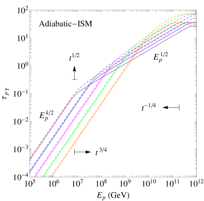
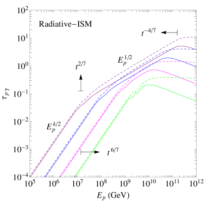
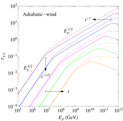
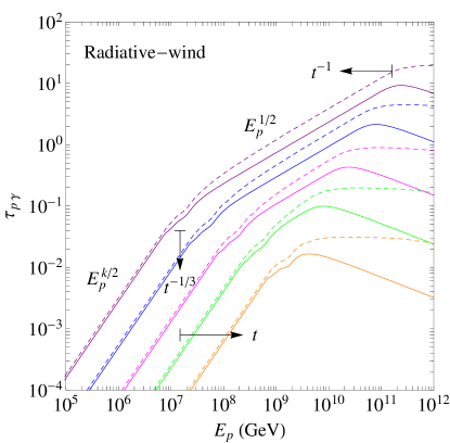
Figure 1: Opacity of $p\gamma$ interactions in the GRB blast wave for cosmic-ray protons which are accelerated by the forward shock. The solid and dashed curves correspond to the opacity calculated by the $\Delta(1232)$ resonance $p\gamma$ cross section and by the full $p\gamma$ cross section, respectively. Each panel corresponds to a particular blast wave evolution scenario. The pairs of solid and dashed curves are calculated, from left to right, at times $t=t_{dec}$, $10t_{dec}$, $10^{2}t_{dec}$, $10^{3}t_{dec}$ and $10^{4}t_{dec}$ for the adiabatic cases (upper panels); and at times $t=t_{dec}$, $3t_{dec}$, $10t_{dec}$, $30t_{dec}$ and $10^{2}t_{dec}$ for the radiative cases (lower panels). Temporal behavior of the break energies [Eq. (14)] and $\tau_{p\gamma}$ at the lower break energy [Eq. (15)] are indicated with labeled arrows. Approximate power-law behavior of different segments of the curves are also indicated. Here we have used $k=2.5$ in Eq. (11).

Figure 1 shows the $p\gamma$ opacity as a function of the cosmic-ray proton energy, as would be observed if they could escape and reach us freely, at different times: $t\geq t_{dec}$ for the 4 different blastwave evolution models, adiabatic and radiative blast waves in the constant density ISM and in the wind of $R^{-2}$ density profile. For the ISM case we have used $\Gamma_{0}=10^{2.8}$ and $n_{0}=1$ whereas in the wind case we have used $\Gamma_{0}=10^{2.6}$ and $A_{\star}=0.1$. The other parameters, common to both cases, are $E_{k}=10^{55}$ erg, $\epsilon_{e}=\epsilon_{B}=0.1$, $\phi=10$, $k=2.5$, $z=1$ and $d_{28}=2.047$. The blast wave deceleration time scales are $10.5$ s and $11.6$ s, respectively, for the ISM and wind cases. The solid lines are for the $\Delta(1232)$ resonance $p\gamma$ cross section and the dashed lines are for the full $p\gamma$ cross section from the SOFIA code Mucke:1999yb . All curves plotted in each blast wave model generally have 2 breaks, the lower (higher) energy break $E_{p,l}$ ($E_{p,h}$) correspnds to the $\varepsilon_{m}$ ($\varepsilon_{c}$) in the synchrotron spectra in Eq. (11). A break at even lower energy corresponding to $\nu_{s}$ is not shown in the plots. As noted in Ref. Razzaque:2006qa , given a target photon spectrum $\varepsilon^{-\alpha}$, the $p\gamma$ opacity for $\Delta(1232)$ resonance cross section scales as $\propto E_{p}^{\alpha-1}$. This behavior is seen for the 3 power-law segments for opacities with the $\Delta(1232)$ resonance cross section and below $E_{p,h}$ for the full cross section. Contributions by additional channels to $\sigma_{p\gamma}$ at $\varepsilon^{\prime}_{r}>\varepsilon^{\prime}_{r,\rm pk}$ affect significantly the $\tau_{p\gamma}$ at $E_{p}\gtrsim E_{p,l}$ because of relatively flatter distributions of target photons below $\varepsilon_{m}$. For $E_{p}\lesssim E_{p,l}$, the $\Delta(1232)$ resonance cross section is still a good approximation for $\tau_{p\gamma}$ (the difference with the full cross section is $\lesssim 10\%$) because of a steeply falling photon spectrum above $\varepsilon_{m}$.

Here we comment in more details about the temporal behavior of the break energies and the opacities as indicated by the arrows in Fig. 1. The break energies can be approximately calculated from the pion production at the energy $\varepsilon^{\prime}_{r,\rm pk}=0.3$ GeV of the peak of the $\Delta(1232)$ cross section, from the condition $\varepsilon^{\prime}_{r}=2\gamma^{\prime}_{p}\varepsilon^{\prime}=\varepsilon^{\prime}_{r,\rm pk}$ as

$$E_{p,l/h}\approx\frac{\varepsilon^{\prime}_{r,\rm pk}\Gamma^{2}}{2\varepsilon_{m/c}(1+z)^{2}}.$$ (14)

These break energies are given in Eqs. (48), (53), (58) and (63) for different blast wave models and for the reference parameters. An approximate analytic expression for the $\tau_{p\gamma}$ optical depth at $E_{p,l}$ can be written as

$$\tau_{p\gamma}(E_{p,l})=\frac{n^{\prime}_{\gamma}(\varepsilon^{\prime}_{m})\varepsilon^{\prime}_{m}\sigma_{\rm pk}R}{2a\Gamma}.$$ (15)

These optical depths are also given in Eqs. (49), (54), (59) and (64) for the 4 different blast wave models that we consider. The agreements between the analytic expressions and the numerical results are very good.

III Neutrino flux calculation

Neutrino flux on the Earth from the GRB blastwave depends on the efficiency of the $p\gamma$ process, as we have discussed above, and on the cosmic-ray density (mostly protons) in the blastwave which we discuss next.

III.1 Cosmic rays in GRB blastwave

The total energy of the cosmic rays in the blastwave, after deceleration ($t>t_{dec}$), is given by

$${\cal E}_{CR}=\begin{cases}\frac{4}{3}\pi\epsilon_{p}n_{0}R^{3}(t)m_{p}c^{2}[\Gamma^{2}(t)-1]&{\rm ISM}\cr 4\pi\epsilon_{p}AR(t)m_{p}c^{2}[\Gamma^{2}(t)-1]&{\rm wind},\end{cases}$$ (16)

in case of a constant density ISM and $R^{-2}$ wind environment, respectively. Here $\epsilon_{p}$ is the fraction of blastwave kinetic energy that goes into accelerated protons. In case of an adiabatic blastwave, either in the ISM or in the wind environment, ${\cal E}_{CR}\approx\epsilon_{p}E_{k}/2$, is constant for $\Gamma(t)\gg 1$. In case of a radiative blastwave, however, ${\cal E}_{CR}$ evolves with time as given in Eqs. (55) and (65), respectively in the ISM and in the wind environment, respectively.

The energy density of cosmic ray protons in the blastwave is therefore $u_{p}={\cal E}_{CR}/V$ in the local rest frame, where $V=(4/3)\pi R^{3}$ is the volume. Acceleration of protons in the GRB blastwave to ultrahigh energies has been discussed in the past Vietri:1995hs . Here we assume that the differential number density of protons, with $n(E_{p})\propto E_{p}^{-2}$ spectrum expected from shock acceleration, is

$$n(E_{p})=\frac{{\cal E}_{CR}}{VE_{p}^{2}{\rm ln}(\gamma^{\prime}_{p,s}/\gamma^{\prime}_{p,m})}.$$ (17)

Here $\gamma^{\prime}_{p,m}=\Gamma$ is the minimum proton Lorentz factor and $\gamma^{\prime}_{p,s}$ is the saturation proton Lorentz factor, both in the comoving blastwave frame. We derive $\gamma^{\prime}_{p,s}$, from the condition that the proton acceleration time $t^{\prime}_{acc}=\phi\gamma^{\prime}_{p}m_{p}c/(eB^{\prime})$ is limited by the dynamic time $t^{\prime}_{dyn}=t\Gamma/(1+z)$, as

$$\gamma^{\prime}_{p,s}(t)=\frac{eB^{\prime}(t)}{\phi m_{p}c}\frac{t\Gamma(t)}{1+z}.$$ (18)

Here $\phi$ is the number of gyroradius required to accelerate proton to the saturation Lorentz factor. An observer would measure an energy $E_{p,s}=\gamma^{\prime}_{p,s}\Gamma/(1+z)$, if these protons could escape the acceleration cite as cosmic rays to reach us, and are given in Eqs. (51), (56), (61) and (66) for the 4 different scenarios that we consider. Note that, in case of strong magnetic field in the blastwave, $t^{\prime}_{acc}$ could be limited by the synchrotron cooling time of the proton $t^{\prime}_{p,syn}=(m_{p}/m_{e})^{3}(6\pi m_{e}c)/(\sigma_{T}B^{\prime 2}\gamma^{\prime}_{p})$, rather than $t^{\prime}_{dyn}$. In such a case the proton saturation Lorentz factor would be given by $\gamma^{\prime}_{p,s}=(m_{p}/m_{e})\sqrt{6\pi e/(\phi\sigma_{T}B^{\prime})}$.

If the cosmic-ray protons could escape freely from the blastwave and avoid interactions with CMB photons, their flux on the Earth would be

$$J_{p}(E_{p})=\frac{c}{4\pi}\left(\frac{R}{d_{L}}\right)^{2}n(E_{p}),$$ (19)

in the zero galactic and intergalactic magnetic field. This flux for the 4 different blaswave scenarios are given in Eq. (52), (57), (62) and (67) with the logarithmic factor in Eq. (17) given by $\xi_{1}={\rm ln}(\gamma^{\prime}_{p,s}/\gamma^{\prime}_{p,m})/10$. Note that all these fluxes decrease with time.

III.2 Neutrino fluxes on the Earth

UHE $\nu$’s from the $p\gamma\to n\pi^{+}$ interactions are produced in two steps, first via $\pi^{+}\to\mu^{+}\nu_{\mu}\to e^{+}\nu_{e}{\bar{\nu}}_{\mu}\nu_{\mu}$ chain decay in the blastwave, and second via neutron beta decay process $n\to pe^{-}{\bar{\nu}}_{e}$ by escaping neutrons from the blastwave while on their way to the Earth. We ignore a small contribution by the $n$-decay flux component in our calculation for simplicity. This component, however, could be important for neutrino flavor ratio calculations. Furthermore we calculate neutrino fluxes from the $\Delta(1232)$ resonance $p\gamma$ cross section, as a conservative estimate. Calculations with the full cross section gives a $\lesssim 30\%$ higher flux in the PeV–EeV range of our interest.

The flux of secondary $\pi^{+}$ or $\pi^{0}$ can be calculated in general, at a time $t\gtrsim t_{dec}$, as

$$J_{\pi}(E_{\pi}) = \int_{0}^{1}\frac{dx}{x}f_{p\to\pi}(x)J_{p}\left(\frac{E_{\pi}}{x}\right)$$ (20)

$$\times K_{p\gamma}\left(\frac{E_{\pi}(1+z)}{x\Gamma}\right)\frac{t\Gamma}{1+z};~{}x=\frac{E_{\pi}}{E_{p}}.$$

Here $K_{p\gamma}$ is evaulated in the blastwave frame. A similar expression can be used for the secondary neutron flux by replacing $\pi\to n$ in the above equation. A simple expression of Eq. (20) follows from the assumption of the pion yield function $f_{p\to\pi}=\delta(x-\langle x\rangle)/2$ for an equal probability of $\pi^{+}$ and $\pi^{0}$ production with a mean inelasticity $\langle x\rangle\approx 0.2$. Therefore, using Eq. (13), we get

$$J_{\pi}(E_{\pi})\approx\frac{1}{2\langle x\rangle}J_{p}\left(\frac{E_{\pi}}{\langle x\rangle}\right)\tau_{p\gamma}\left(\frac{E_{\pi}(1+z)}{\langle x\rangle\Gamma}\right),$$ (21)

for $\tau_{p\gamma}\leq 1$. For the neutron flux, $J_{n}(E_{n})$, the mean inelasticity is $\langle x\rangle\approx 0.8$.

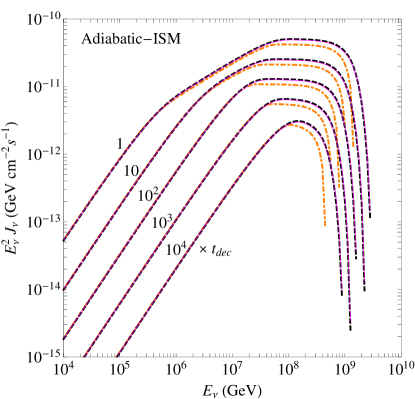
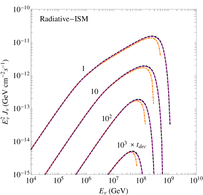
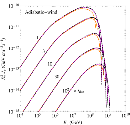
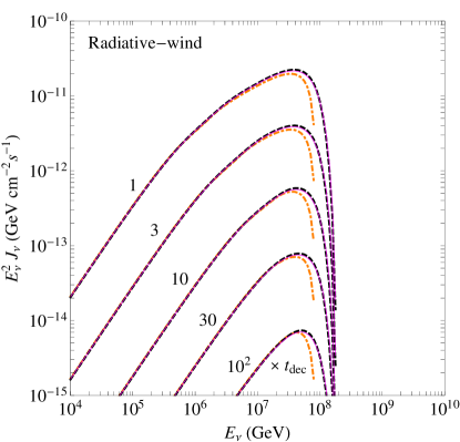
Figure 2: Neutrino fluxes from a GRB at redshift $z=1$ for 4 different blastwave models. The model parameters are the same as in Fig. 1 for each case: $\Gamma_{0}=10^{2.8}$ and $n_{0}=1$ for the ISM ($t_{dec}=10.5$ s); $\Gamma_{0}=10^{2.6}$ and $A_{\star}=0.1$ for the wind ($t_{dec}=11.6$ s); the common parameters are $E_{k}=10^{55}$ erg, $\epsilon_{p}=1$, $\epsilon_{e}=\epsilon_{B}=0.1$, $\phi=10$, $k=2.5$ and $d_{L}=2.047\times 10^{28}$ cm. The dotted-dash lines are for $\nu_{\mu}$ fluxes from $\pi^{+}$ decay, the solid lines are for ${\bar{\nu}}_{\mu}$ fluxes from $\mu^{+}$ decay and the dashed lines are for $\nu_{e}$ fluxes from $\mu^{+}$ decay. Neutrino oscillation has not been taken into account for the plotted fluxes.

The muon and muon neutrino (pionic neutrino) fluxes from the pion decay $\pi^{+}\to\mu^{+}\nu_{\mu}$ are given by

$$J_{\mu}(E_{\mu}) = \int_{0}^{1}\frac{dx}{x}f_{\pi^{+}\to\mu^{+}}(x)J_{\pi}\left(\frac{E_{\mu}}{x}\right);~{}x=\frac{E_{\mu}}{E_{\pi}},$$

$$J_{\nu_{\mu}}(E_{\nu}) = \int_{0}^{1}\frac{dx}{x}f_{\pi^{+}\to\nu_{\mu}}(x)J_{\pi}\left(\frac{E_{\nu}}{x}\right);~{}x=\frac{E_{\nu}}{E_{\pi}}.~{}~{}$$ (22)

where the scaling functions $f_{\pi^{+}\to\mu^{+}}$ and $f_{\pi^{+}\to\nu_{\mu}}$ are given by Eq. (68), following Ref. Lipari:1993hd . The subsequent $\nu$ fluxes (muonic neutrinos) from the $\mu^{+}\to e^{+}\nu_{e}{\bar{\nu}}_{\mu}$ decay are given by

$$J_{\nu_{e}}(E_{\nu}) = \int_{0}^{1}\frac{dy}{y}\int_{0}^{1}\frac{dx}{x}f_{\mu^{+}\to\nu_{e}}(x,y)f_{\pi\to\mu}(x)$$

$$\times J_{\pi}\left(\frac{E_{\nu}}{xy}\right);~{}x=\frac{E_{\mu}}{E_{\pi}},~{}y=\frac{E_{\nu}}{E_{\mu}},$$

$$J_{{\bar{\nu}}_{\mu}}(E_{\nu}) = \int_{0}^{1}\frac{dy}{y}\int_{0}^{1}\frac{dx}{x}f_{\mu^{+}\to{\bar{\nu}}_{\mu}}(x,y)f_{\pi\to\mu}(x)$$ (23)

$$\times J_{\pi}\left(\frac{E_{\nu}}{xy}\right);~{}x=\frac{E_{\mu}}{E_{\pi}},~{}y=\frac{E_{\nu}}{E_{\mu}},$$

The scaling functions $f_{\mu^{+}\to\nu_{e}}$ and $f_{\mu^{+}\to{\bar{\nu}}_{\mu}}$ from Ref. Lipari:1993hd are given in Eq. (70) for completeness.

Figure 2 shows $\nu$ fluxes from a GRB at redshift $z=1$ for the 4 different blastwave evolution models that we have considered. The fluxes are calculated at the same time as for the respective $\tau_{p\gamma}$ plots in Fig. 1. The fluxes for the adiabatic blastwave in the wind environment at $t_{dec}=11.6$ s are the highest among all 4 blastwave models, in the PeV–EeV range. On the other hand, significantly high fluxes from an adiabatic blastwave in the ISM environment last for the longest time. Fluxes from a radiative blastwave, either in the ISM or wind environment, decrease faster than the fluxes from an adiabatic fireball, as the $p\gamma$ opacity also dcereases faster in the radiative blastwaves (Fig. 1). Plotted fluxes in Fig. 2 are the “source fluxes” without taking into account neutrino oscillation. To a good approximation, the $\nu_{e}+{\bar{\nu}}_{e}$, $\nu_{\mu}+{\bar{\nu}}_{\mu}$ and $\nu_{\tau}+{\bar{\nu}}_{\tau}$ fluxes at a detector on the Earth will be equal to the plotted ${\bar{\nu}}_{\mu}$ flux in Fig. 2.

It is not straightforward to estimate the diffuse fluxes of neutrinos from the GRB blastwave models we have considered, because of the unknown rate of these bursts. Our models are motivated by the Fermi-LAT detection of delayed emission of GeV photons from GRBs. Such delays are explained as forward-shock synchrotron emission Kumar:2009vx ; Ghisellini+10 ; Razzaque:2010ku , requiring $\sim 10$ s time scale for long-duration GRB fireball with high bulk Lorentz factor to decelerate. Detection of GRBs by Fermi-LAT during its operation since launch in 2008 suggests that the rate of the GeV bright GRBs is likely lower than the rate of typical GRBs Fermi-LAT:2013kxa .

In Figure 3 we roughly estimate the diffuse $\nu$ fluxes as follows. We calculate the time-integrated flux from the fluxes plotted in Fig. 2 for each of the blastwave models. We assume the rate of these GRBs, placed at redshift $z=1$, is 2/day over the whole sky and cosmological source evolution gives a multiplicative factor of 3. To show the uncertainty of the rate of GRBs with high bulk Lorentz factor, we have plotted the diffuse fluxes assuming that $100\%$ and $10\%$ of the GRBs have the same characteristics used in modeling. These are indicatives of the rates detected by Fermi-GBM and Fermi-LAT, respectively. The plotted $\nu_{\mu}+{\bar{\nu}}_{\mu}$ fluxes are calculated by taking into account neutrino oscillation in vacuum, which gives nearly equal fluxes of the 3 flavors. Note that the diffuse $\nu$ flux from the adibatic blastwave in ISM dominates the flux models, as expected from the longest-lived emission in this scenario. We have also shown the recently published IceCube upper limit on the GRB prompt $\nu$ flux Abbasi:2012zw . Notably our $\nu$ flux models are consistent with this limit, except for the adiabatic blastwave in the ISM case at $\sim 1$–3 PeV. This might have interesting consequences with regards to the recent discovery of two neutrino events at $\sim 1$ PeV Aartsen:2013bka by the IceCube Neutrino Observatory Ahrens:2003ix .

Figure 3: Diffuse $\nu_{\mu}+{\bar{\nu}}_{\mu}$ fluxes from GRB blastwave in 4 different evolution scenarios. The top and bottom lines of the same type, with shaded region in between, correspond to $100\%$ and $10\%$ of the GRBs having high bulk Lorentz factors. Also shown is the recent upper limit on GRB internal shock $\nu$ flux model Waxman:1997ti from IceCube Abbasi:2012zw . Neutrino oscillation in vacuum has been taken into account for the diffuse flux models, which leads to equal fluxes of $\nu_{e}+{\bar{\nu}}_{e}$ and $\nu_{\tau}+{\bar{\nu}}_{\tau}$ as the $\nu_{\mu}+{\bar{\nu}}_{\mu}$ flux plotted here.

IV Detection prospects

It was pointed out sometime ago that the burst-to-burst fluctuation may result in single GRBs to dominate the diffuse flux AlvarezMuniz:2000st . Moreover, only a few neutrinos might be detected by IceCube, in the optimistic Waxman-Bahcall scenario Waxman:1997ti , for a very nearby burst such as GRB 030329 Razzaque:2003uw at redshift $z=0.17$. It is unlikely that the two $\sim 1$ PeV events detected by IceCube originated from very nearby GRBs, using the flux models presented here and given the average neutrino effective area ($\sim 10$ m² at $\sim 1$ PeV for the combined 3 flavors) of the detector when these two events were detected Aartsen:2013bka .

The combined diffuse flux of all 3 $\nu$ flavors in case of the adiabatic blastwave in ISM (Fig. 3) is $\sim 6\times 10^{-9}$ GeV cm^-2 s^-1 sr^-1 at 1 PeV. A $\sim 6$ times higher cosmological GRB rate than the 2/day that we have used or a $\sim 6$ times higher kinetic energy per burst could in principle produce the $3.6\times 10^{-8}$ GeV cm^-2 s^-1 sr^-1 diffuse neutrino flux model required by IceCube to generate the two $\sim 1$ PeV events Aartsen:2013bka . Note that this required diffuse flux is higher than the Waxman-Bahcall limit Waxman:1998yy .

The prosepects for detection of PeV–EeV neutrinos from GRB blastwaves that we have modeled, are much better for the future 100 km³ radio Askaryan detectors in Antarctica such as ARIANNA Barwick:2006tg and ARA Allison:2011wk . A few PeV–EeV neutrinos can be detected by these experiments from nearby GRBs according to our flux models. Our diffuse $\nu$ flux for the adiabatic-ISM scenario should be detectable by ARIANNA or ARA within 3 years of their operation.

V Discussion and conclusions

We have calculated new, realistic $\nu$ fluxes from GRB blastwave models, which are responsible for radio to X-ray afterglow and possibly GeV $\gamma$-ray emission. A very-high bulk Lorentz factor of the GRB jet, which adversely affects the $\nu$ production efficiency in the internal shocks, works favorably in our scenario by shortening the afterglow onset time and by producing a bright afterglow which provide ample target photons for $p\gamma$ interactions. The long-lived PeV–EeV $\nu$ emission is due to $p\gamma$ interactions of protons, accelerated to UHE in the forward shock of the blastwave, with afterglow photons. These $\nu$ fluxes from the external forward shock should be present in the GRB afterglow, if protons are co-accelerated with electrons, even if the prompt $\gamma$ rays are produced by a different mechanism than the internal shocks and/or if the external reverse shock is absent, e.g. in case of a Poynting flux dominated GRB ejecta.

We have computed $\nu$ fluxes for 4 different blastwave evolution scenarios, namely adiabatic and fully radiative blastwaves in a constant density ISM environment and in an environment with $R^{-2}$ wind density profile. The PeV–EeV $\nu$ fluxes peak at the blastwave deceleration time and decrease after that in all the cases, as the $p\gamma$ interaction efficiency decreases with the increasing blastwave radius, and as the protons are less efficiently accelerated to UHE with increasing time. Neutrino fluxes from the adiabatic blastwaves last longer than the radiative ones, as expected, with the adiabatic-ISM scenario being the longest lasting case. The diffuse $\nu$ fluxes that we have calculated depend on the unknown rate of the high bulk Lorentz factor bursts. The diffuse $\nu$ flux from an adiabatic blastwave in ISM is the highest among all the models.

The interpretation of the two $\sim 1$ PeV $\nu$ events detected by IceCube does not follow naturally from our diffuse flux models but could be accommodated in very optimistic scenario with higher GRB rate and/or higher kinetic energy per GRB than we have considered. Detection of the PeV–EeV $\nu$ from the GRB afterglow that we have predicted could be possible by upcoming, large radio Askaryan detectors in Antarctica and verify the hypothesis of UHECR acceleration in the GRB blastwave.

Appendix A Blastwave models and synchrotron spectra

In the following, we provide the bulk Lorentz factor and radius of the blastwave along with the shock magnetic field in four different evolution scenarios described in Eqs. (3) and (4). We also list the break frequencies ($h\nu_{c}$, $h\nu_{m}$, $h\nu_{s}$) in the synchrotron spectrum, the time scale ($t_{0}$) for which the fast-cooling regime is valid and the maximum synchrotron flux ($F_{\nu,m}$), to facilitate calculation of the target photon spectrum for $p\gamma$ interactions in the GRB blastwave frame. We have assumed the parameters $\epsilon_{B}=0.1\epsilon_{B,-1}$, $\epsilon_{e}=0.1\epsilon_{e,-1}$ from typical GRB afterglow modeling, $10\phi_{1}$ gyroradius to accelerate particles and a reference time $t=10^{2}t_{2}$ s.

A.1 Adiabatic blastwave in ISM

$$\Gamma=124\,(1+z)^{3/8}n_{0}^{-1/8}E_{55}^{1/8}t_{2}^{-3/8}.$$ (24)

$$R=3.7\times 10^{17}(1+z)^{-1/4}n_{0}^{-1/4}E_{55}^{1/4}t_{2}^{1/4}~{}{\rm cm}.$$ (25)

$$B^{\prime}=15.3\,(1+z)^{3/8}\epsilon_{B,-1}^{1/2}n_{0}^{3/8}E_{55}^{1/8}t_{2}^{-3/8}~{}{\rm G}.$$ (26)

$$h\nu_{c} = 2.3\,(1+z)^{-1/2}\epsilon_{B,-1}^{-3/2}n_{0}^{-1}E_{55}^{-1/2}t_{2}^{-1/2}~{}{\rm eV},$$

$$h\nu_{m} = 17.3\,(1+z)^{1/2}\epsilon_{B,-1}^{1/2}\epsilon_{e,-1}^{2}E_{55}^{1/2}t_{2}^{-3/2}~{}{\rm keV},$$

$$h\nu_{s} = 2.9\,(1+z)^{-5/8}\phi_{1}^{-1}n_{0}^{-1/8}E_{55}^{1/8}t_{2}^{-3/8}~{}{\rm GeV}.$$ (27)

$$t_{0}=1.1\times 10^{7}(1+z)\epsilon_{B,-1}^{2}\epsilon_{e,-1}^{2}n_{0}E_{55}~{}{\rm s}.$$ (28)

$$F_{\nu,m}=8.2\,(1+z)^{-1}\epsilon_{B,-1}^{1/2}n_{0}^{1/2}E_{55}d_{28}^{-2}~{}{\rm Jy}.$$ (29)

A.2 Radiative blastwave in ISM

$$\Gamma=86\,(1+z)^{3/7}n_{0}^{-1/7}\Gamma_{2.5}^{-1/7}E_{55}^{1/7}t_{2}^{-3/7}.$$ (30)

$$R=3.1\times 10^{17}(1+z)^{-1/7}n_{0}^{-2/7}\Gamma_{2.5}^{-2/7}E_{55}^{2/7}t_{2}^{1/7}~{}{\rm cm}.$$ (31)

$$B^{\prime}=10.5\,(1+z)^{3/7}\epsilon_{B,-1}^{1/2}n_{0}^{5/14}\Gamma_{2.5}^{-1/7}E_{55}^{1/7}t_{2}^{-3/7}~{}{\rm G}.$$ (32)

$$h\nu_{c} = 10.4\,(1+z)^{-5/7}\epsilon_{B,-1}^{-3/2}n_{0}^{-13/14}\Gamma_{2.5}^{4/7}E_{55}^{-4/7}t_{2}^{-2/7}~{}{\rm eV},$$

$$h\nu_{m} = 4.0\,(1+z)^{5/7}\epsilon_{B,-1}^{1/2}\epsilon_{e,-1}^{2}n_{0}^{-1/14}\Gamma_{2.5}^{-4/7}E_{55}^{4/7}t_{2}^{-12/7}~{}{\rm keV},$$

$$h\nu_{s} = 2.0\,(1+z)^{-4/7}\phi_{1}^{-1}n_{0}^{-1/7}\Gamma_{2.5}^{-1/7}E_{55}^{1/7}t_{2}^{-3/7}~{}{\rm GeV}.$$ (33)

$$t_{0} = 6.3\times 10^{3}(1+z)\epsilon_{B,-1}^{7/5}\epsilon_{e,-1}^{7/5}n_{0}^{3/5}\Gamma_{2.5}^{-4/5}E_{55}^{4/5}~{}{\rm s}.$$ (34)

$$F_{\nu,m}=2.2\,(1+z)^{-4/7}\epsilon_{B,-1}^{1/2}n_{0}^{5/14}\Gamma_{2.5}^{-8/7}E_{55}^{8/7}t_{2}^{-3/7}d_{28}^{-2}~{}{\rm Jy}.$$ (35)

A.3 Adiabatic blastwave in wind

$$\Gamma=78\,(1+z)^{1/4}A_{\star}^{-1/4}E_{55}^{1/4}t_{2}^{-1/4}.$$ (36)

$$R=1.4\times 10^{17}(1+z)^{-1/2}A_{\star}^{-1/2}E_{55}^{1/2}t_{2}^{1/2}~{}{\rm cm}.$$ (37)

$$B^{\prime}=9.5\,(1+z)^{1/4}\epsilon_{B,-1}^{1/2}A_{\star}^{1/4}E_{55}^{1/4}t_{2}^{-1/4}~{}{\rm G}.$$ (38)

$$h\nu_{c} = 0.3\,(1+z)^{-3/2}\epsilon_{B,-1}^{-3/2}A_{\star}^{-2}E_{55}^{1/2}t_{2}^{1/2}~{}{\rm eV},$$

$$h\nu_{m} = 10.0\,(1+z)^{1/2}\epsilon_{B,-1}^{1/2}\epsilon_{e,-1}^{2}E_{55}^{1/2}t_{2}^{-3/2}~{}{\rm keV},$$

$$h\nu_{s} = 1.8\,(1+z)^{-3/4}\phi_{1}^{-1}A_{\star}^{-1/4}E_{55}^{1/4}t_{2}^{-1/4}~{}{\rm GeV}.$$ (39)

$$t_{0}=1.9\times 10^{4}(1+z)\epsilon_{B,-1}\epsilon_{e,-1}A_{\star}~{}{\rm s}.$$ (40)

$$F_{\nu_{m}} = 10.4\,(1+z)^{-1/2}\epsilon_{B,-1}^{1/2}A_{\star}E_{55}^{1/2}t_{2}^{-1/2}d_{28}^{-2}~{}{\rm Jy}.$$ (41)

A.4 Radiative blastwave in wind

$$\Gamma=40\,(1+z)^{1/3}A_{\star}^{-1/3}\Gamma_{2.5}^{-1/3}E_{55}^{1/3}t_{2}^{-1/3}.$$ (42)

$$R=6.9\times 10^{16}(1+z)^{-1/3}A_{\star}^{-2/3}\Gamma_{2.5}^{-2/3}E_{55}^{2/3}t_{2}^{2/3}~{}{\rm cm}.$$ (43)

$$B^{\prime}=5.0\,(1+z)^{1/3}\epsilon_{B,-1}^{1/2}A_{\star}^{1/6}\Gamma_{2.5}^{-1/3}E_{55}^{1/3}t_{2}^{-1/3}~{}{\rm G}.$$ (44)

$$h\nu_{c} = 0.4\,(1+z)^{-4/3}\epsilon_{B,-1}^{-3/2}A_{\star}^{-13/6}\Gamma_{2.5}^{-2/3}E_{55}^{2/3}t_{2}^{1/3}~{}{\rm eV},$$

$$h\nu_{m} = 1.5\,(1+z)^{2/3}\epsilon_{B,-1}^{1/2}\epsilon_{e,-1}^{2}A_{\star}^{-1/6}\Gamma_{2.5}^{-2/3}E_{55}^{2/3}t_{2}^{-5/3}~{}{\rm keV},$$

$$h\nu_{s} = 1.0\,(1+z)^{-2/3}\phi_{1}^{-1}A_{\star}^{-1/3}\Gamma_{2.5}^{-1/3}E_{55}^{1/3}t_{2}^{-1/3}~{}{\rm GeV}.$$ (45)

$$t_{0}=6.1\times 10^{3}(1+z)\epsilon_{B,-1}\epsilon_{e,-1}A_{\star}\,{\rm s}.$$ (46)

$$F_{\nu_{m}} = 2.8\,(1+z)^{-1/3}\epsilon_{B,-1}^{1/2}A_{\star}^{5/6}\Gamma_{2.5}^{-2/3}E_{55}^{2/3}t_{2}^{-2/3}d_{28}^{-2}~{}{\rm Jy}.$$ (47)

Appendix B $p\gamma$ interaction and cosmic-ray parameters

Here we provide numerical values for the break energies in Eq. (14), the optical depth in Eq. (15), the total energy in cosmic rays given by Eq. (16), the limiting cosmic-ray energy in Eq. (18) and the cosmic-ray flux in Eq. (19) for the 4 different blast wave models.

B.1 Adiabatic blastwave in ISM

$$E_{p,l} = 1.3\times 10^{8}(1+z)^{-7/4}\epsilon_{B,-1}^{-1/2}\epsilon_{e,-1}^{-2}n_{0}^{-1/4}E_{55}^{-1/4}t_{2}^{3/4}~{}{\rm GeV},$$

$$E_{p,h} = 1.0\times 10^{12}(1+z)^{-3/4}\epsilon_{B,-1}^{3/2}n_{0}^{3/4}E_{55}^{3/4}t_{2}^{-1/4}~{}{\rm GeV}.$$ (48)

$$\tau_{p\gamma}(E_{p,l})=0.7\,(1+z)^{-1/2}\epsilon_{B,-1}^{1/2}n_{0}E_{55}^{1/2}t_{2}^{1/2}.$$ (49)

$${\cal E}_{CR}=\epsilon_{p}E_{k}/2.$$ (50)

$$E_{p,s}=2.3\times 10^{19}(1+z)^{-7/8}\phi_{1}^{-1}n_{0}^{1/8}\epsilon_{B,-1}^{1/2}E_{55}^{3/8}t_{2}^{-1/8}~{}{\rm eV}.$$ (51)

$$E_{p}^{2}J_{p}(E_{p})=4.8\times 10^{-9}(1+z)^{1/4}\xi_{1}^{-1}\epsilon_{p}n_{0}^{1/4}E_{55}^{3/4}t_{2}^{-1/4}d_{28}^{-2}~{}{\rm GeV~{}cm}^{-2}~{}{\rm s}^{-1}.$$ (52)

B.2 Radiative blastwave in ISM

$$E_{p,l} = 2.8\times 10^{8}(1+z)^{-13/7}\epsilon_{B,-1}^{-1/2}\epsilon_{e,-1}^{-2}n_{0}^{-3/14}\Gamma_{2.5}^{2/7}E_{55}^{-2/7}t_{2}^{6/7}~{}{\rm GeV},$$

$$E_{p,h} = 1.1\times 10^{11}(1+z)^{-3/7}\epsilon_{B,-1}^{3/2}n_{0}^{9/14}\Gamma_{2.5}^{-6/7}E_{55}^{6/7}t_{2}^{-4/7}~{}{\rm GeV}.$$ (53)

$$\tau_{p\gamma}(E_{p,l})=0.5\,(1+z)^{-2/7}\epsilon_{B,-1}^{1/2}n_{0}^{13/14}\Gamma_{2.5}^{-4/7}E_{55}^{4/7}t_{2}^{2/7}.$$ (54)

$${\cal E}_{CR}=1.4\times 10^{54}(1+z)^{3/7}\epsilon_{p}n_{0}^{-1/7}\Gamma_{2.5}^{-8/7}E_{55}^{8/7}t_{2}^{-3/7}~{}{\rm erg}.$$ (55)

$$E_{p,s}=7.4\times 10^{18}(1+z)^{-5/7}\phi_{1}^{-1}\epsilon_{B,-1}^{1/2}n_{0}^{1/14}\Gamma_{2.5}^{-3/7}E_{55}^{3/7}t_{2}^{-2/7}~{}{\rm eV}.$$ (56)

$$E_{p}^{2}J_{p}(E_{p})=1.6\times 10^{-9}(1+z)^{4/7}\xi_{1}^{-1}\epsilon_{p}n_{0}^{1/7}\Gamma_{2.5}^{-6/7}E_{55}^{6/7}t_{2}^{-4/7}d_{28}^{-2}~{}{\rm GeV~{}cm}^{-2}~{}{\rm s}^{-1}.$$ (57)

B.3 Adiabatic blastwave in wind

$$E_{p,l} = 9.1\times 10^{7}(1+z)^{-2}\epsilon_{B,-1}^{-1/2}\epsilon_{e,-1}^{-2}A_{\star}^{-1/2}t_{2}~{}{\rm GeV},$$

$$E_{p,h} = 3.2\times 10^{12}\epsilon_{B,-1}^{3/2}A_{\star}^{3/2}t_{2}^{-1}~{}{\rm GeV}.$$ (58)

$$\tau_{p\gamma}(E_{p,l})=6.0\,(1+z)^{1/2}\epsilon_{B,-1}^{1/2}A_{\star}^{2}E_{55}^{-1/2}t_{2}^{-1/2}.$$ (59)

$${\cal E}_{CR}=\epsilon_{p}E_{k}/2.$$ (60)

$$E_{p,s}=6\times 10^{18}(1+z)^{-5/4}\phi_{1}^{-1}A_{\star}^{-1/4}\epsilon_{B,-1}^{1/2}E_{55}^{3/4}t_{2}^{1/4}~{}{\rm eV}.$$ (61)

$$E_{p}^{2}J_{p}(E_{p})=1.2\times 10^{-8}(1+z)^{1/2}\xi_{1}^{-1}\epsilon_{p}A_{\star}^{1/2}E_{55}^{1/2}t_{2}^{-1/2}d_{28}^{-2}~{}{\rm GeV~{}cm}^{-2}~{}{\rm s}^{-1}.$$ (62)

B.4 Radiative blastwave in wind

$$E_{p,l} = 1.6\times 10^{8}(1+z)^{-2}\epsilon_{B,-1}^{-1/2}\epsilon_{e,-1}^{-2}A_{\star}^{-1/2}t_{2}~{}{\rm GeV},$$

$$E_{p,h} = 6.0\times 10^{11}\epsilon_{B,-1}^{3/2}A_{\star}^{3/2}t_{2}^{-1}~{}{\rm GeV}.$$ (63)

$$\tau_{p\gamma}(E_{p,l})=12.6\,(1+z)^{1/3}\epsilon_{B,-1}^{1/2}A_{\star}^{13/6}\Gamma_{2.5}^{2/3}E_{55}^{-2/3}t_{2}^{-1/3}.$$ (64)

$${\cal E}_{CR}=6.4\times 10^{53}(1+z)^{1/3}\epsilon_{p}A_{\star}^{1/3}\Gamma_{2.5}^{-4/3}E_{55}^{4/3}t_{2}^{-1/3}~{}{\rm erg}.$$ (65)

$$E_{p,s}=8\times 10^{17}(1+z)^{-1}\phi_{1}^{-1}\epsilon_{B,-1}^{1/2}A_{\star}^{-1/2}\Gamma_{2.5}^{-1}E_{55}~{}{\rm eV}.$$ (66)

$$E_{p}^{2}J_{p}(E_{p})=3.3\times 10^{-9}(1+z)^{2/3}\xi_{1}^{-1}\epsilon_{p}A_{\star}^{1/3}\Gamma_{2.5}^{-2/3}E_{55}^{2/3}t_{2}^{-2/3}d_{28}^{-2}~{}{\rm GeV~{}cm}^{-2}~{}{\rm s}^{-1}.$$ (67)

Appendix C Pion and muon decay scaling functions

For completeness, we quote here the spectra of secondary particles, called scaling functions, for the pion and muon decays given in Ref. Lipari:1993hd . In terms of the ratio between the muon and pion masses squared: $r_{\pi}=m_{\mu}^{2}/m_{\pi}^{2}$, the pion decay scaling relations are

$$f_{\pi\to\mu}(x) = \frac{1}{1-r_{\pi}}\Theta(x-r_{\pi}),$$

$$f_{\pi\to\nu_{\mu}}(x) = \frac{1}{1-r_{\pi}}\Theta(1-r_{\pi}-x).$$ (68)

Note that pion decay muons are polarized and one should take into account their helicities (negative for $\mu^{+}$ and positive for $\mu^{-}$, on the average) since the neutrino spectra from muon decay depend on the polarization. The helicity function, in case of ultra-relativistic pion decay, is given by

$$P_{\pi^{\pm}\to\mu^{\pm}}(x)=\pm\frac{2r_{\pi}}{x(1-r_{\pi})}\mp\frac{1+r_{\pi}}{1-r_{\pi}}.$$ (69)

The muon decay scaling relations are

$$f_{\mu^{+}\to\nu_{e}}(x,y) = (2-6y^{2}+4y^{3})+P_{\pi^{+}\to\mu^{+}}(x)(-2+12y-18y^{2}+8y^{3}),$$

$$f_{\mu^{+}\to{\bar{\nu}}_{\mu}}(x,y) = \left(\frac{5}{3}-3y^{2}+\frac{4}{3}y^{3}\right)+P_{\pi^{+}\to\mu^{+}}(x)\left(\frac{1}{3}-3y^{2}+\frac{8}{3}y^{3}\right).$$ (70)

References

(1)
A. MacFadyen and S. E. Woosley,
Astrophys. J. 524, 262 (1999)
[astro-ph/9810274].
(2)
S. Woosley and A. Heger,
Astrophys. J. 637, 914 (2006)
[astro-ph/0508175].
(3)
P. Meszaros, P. Laguna and M. J. Rees,
Astrophys. J. 415, 181 (1993)
[astro-ph/9301007].
(4)
M. J. Rees and P. Meszaros,
Astrophys. J. 430, L93 (1994)
[astro-ph/9404038].
(5)
T. Piran,
Rev. Mod. Phys. 76, 1143 (2004)
[astro-ph/0405503].
(6)
B. Zhang and P. Meszaros,
Int. J. Mod. Phys. A 19, 2385 (2004)
[astro-ph/0311321].
(7)
E. Waxman,
Phys. Rev. Lett. 75, 386 (1995)
[astro-ph/9505082].
(8)
E. Waxman and J. N. Bahcall,
Phys. Rev. Lett. 78, 2292 (1997)
[astro-ph/9701231].
(9)
R. Abbasi et al. [IceCube Collaboration],
Nature 484, 351 (2012)
[arXiv:1204.4219 [astro-ph.HE]].
(10)
S. Adri n-Mart nez, A. Albert, I. A. Samarai, M. Andr , M. Anghinolfi, G. Anton, S. Anvar and M. Ardid et al.,
arXiv:1307.0304 [astro-ph.HE].
(11)
C. D. Dermer and A. Atoyan,
Phys. Rev. Lett. 91, 071102 (2003)
[astro-ph/0301030].
(12)
K. Murase and S. Nagataki,
Phys. Rev. D 73, 063002 (2006)
[astro-ph/0512275].
(13)
S. Hummer, P. Baerwald and W. Winter,
Phys. Rev. Lett. 108, 231101 (2012)
[arXiv:1112.1076 [astro-ph.HE]].
(14)
N. Gehrels and S. Razzaque,
Invited review article in the special issue of Frontiers of Physics on High Energy Astrophysics, eds. B. Zhang and P. Meszaros,
arXiv:1301.0840 [astro-ph.HE].
(15)
W. B. Atwood et al. [LAT Collaboration],
Astrophys. J. 697, 1071 (2009)
[arXiv:0902.1089 [astro-ph.IM]].
(16)
R. D. Blandford and C. F. McKee,
Phys. Fluids 19, 1130 (1976).
(17)
P. Meszaros and M. J. Rees,
Astrophys. J. 476, 232 (1997)
[astro-ph/9606043].
(18)
R. ’e. Sari, T. Piran and R. Narayan,
Astrophys. J. 497, L17 (1998)
[astro-ph/9712005].
(19)
M. De Pasquale et al. [Fermi-LAT and GBM Collaborations],
Astrophys. J. 709, L146 (2010)
[arXiv:0910.1629 [astro-ph.HE]].
(20)
M. Ackermann et al. [Fermi-LAT and GBM Collaborations],
Astrophys. J. 763, 71 (2013)
[arXiv:1212.0973 [astro-ph.HE]].
(21)
P. Kumar and R. B. Duran,
Mon. Not. Roy. Astron. Soc. 409, 226 (2010)
[arXiv:0910.5726 [astro-ph.HE]].
(22)
G. Ghisellini, G. Ghirlanda, L. Nava & A. Celotti,
Mon. Not. Roy. Astron. Soc. 403, 926 (2010)
(23)
T. Piran and E. Nakar,
Astrophys. J. 718, L63 (2010)
[arXiv:1003.5919 [astro-ph.HE]].
(24)
W. B. Atwood, L. Baldini, J. Bregeon, P. Bruel, A. Chekhtman, J. Cohen-Tanugi, A. Drlica-Wagner and J. Granot et al.,
Astrophys. J. (in press)
arXiv:1307.3037 [astro-ph.HE].
(25)
S. Razzaque, C. D. Dermer and J. D. Finke,
Open Astron. J. 3, 150 (2010)
[arXiv:0908.0513 [astro-ph.HE]].
(26)
S. Razzaque,
Astrophys. J. 724, L109 (2010)
[arXiv:1004.3330 [astro-ph.HE]].
(27)
M. Vietri,
Astrophys. J. 453, 883 (1995)
[astro-ph/9506081].
(28)
E. Waxman and J. N. Bahcall,
Astrophys. J. 541, 707 (2000)
[hep-ph/9909286].
(29)
Z. G. Dai and T. Lu,
Astrophys. J. 551, 249 (2001)
(30)
K. Murase,
Phys. Rev. D 76, 123001 (2007)
[arXiv:0707.1140 [astro-ph]].
(31)
J. A. Nousek, C. Kouveliotou, D. Grupe, K. Page, J. Granot, E. Ramirez-Ruiz, S. K. Patel and D. N. Burrows et al.,
Astrophys. J. 642, 389 (2006)
[astro-ph/0508332].
(32)
B. Zhang, Y. Z. Fan, J. Dyks, S. Kobayashi, P. Meszaros, D. N. Burrows, J. A. Nousek and N. Gehrels,
Astrophys. J. 642, 354 (2006)
[astro-ph/0508321].
(33)
C. D. Dermer,
Astrophys. J. 574, 65 (2002)
[astro-ph/0005440].
(34)
Z. Li, Z. G. Dai and T. Lu,
Astron. Astrophys. 396, 303 (2002)
[astro-ph/0208435].
(35)
R. A. Chevalier and Z.-Y. Li,
Astrophys. J. 536, 195 (2000)
[astro-ph/9908272].
(36)
J. Granot and R. ’e. Sari,
Astrophys. J. 568, 820 (2002)
[astro-ph/0108027].
(37)
A. Panaitescu and P. Kumar,
Astrophys. J. 560, L49 (2001)
[astro-ph/0108045].
(38)
A. Mucke, R. Engel, J. P. Rachen, R. J. Protheroe and T. Stanev,
Comput. Phys. Commun. 124, 290 (2000)
[astro-ph/9903478].
(39)
S. Razzaque, J. A. Adams, P. Harris and D. Besson,
Astropart. Phys. 26, 367 (2007)
[astro-ph/0605480].
(40)
P. Lipari,
Astropart. Phys. 1, 195 (1993).
(41)
M. Ackermann et al. [Fermi-LAT Collaboration],
Astrophys. J. (submitted)
arXiv:1303.2908 [astro-ph.HE].
(42)
J. Alvarez-Muniz, F. Halzen and D. W. Hooper,
Phys. Rev. D 62, 093015 (2000)
[astro-ph/0006027].
(43)
J. Ahrens et al. [IceCube Collaboration],
Astropart. Phys. 20, 507 (2004)
[astro-ph/0305196].
(44)
S. Razzaque, P. Meszaros and E. Waxman,
Phys. Rev. D 69, 023001 (2004)
[astro-ph/0308239].
(45)
M. G. Aartsen et al. [IceCube Collaboration],
Phys. Rev. Lett. 111, 021103 (2013)
[arXiv:1304.5356 [astro-ph.HE]].
(46)
E. Waxman and J. N. Bahcall,
Phys. Rev. D 59, 023002 (1999)
[hep-ph/9807282].
(47)
S. W. Barwick,
J. Phys. Conf. Ser. 60, 276 (2007)
[astro-ph/0610631].
(48)
P. Allison, J. Auffenberg, R. Bard, J. J. Beatty, D. Z. Besson, S. Boser, C. Chen and P. Chen et al.,
Astropart. Phys. 35, 457 (2012)
[arXiv:1105.2854 [astro-ph.IM]].