The XMM-Newton survey of the Small Magellanic Cloud:
The X-ray point-source catalogue

Abstract

Context. Local-Group galaxies provide access to samples of X-ray source populations of whole galaxies. The XMM-Newton survey of the Small Magellanic Cloud (SMC) completely covers the bar and eastern wing with a 5.6 deg² area in the (0.2$-$12.0) keV band.

Aims. To characterise the X-ray sources in the SMC field, we created a catalogue of point sources and sources with moderate extent. Sources with high extent ($\geq$40″) have been presented in a companion paper.

Methods. We searched for point sources in the EPIC images using sliding-box and maximum-likelihood techniques and classified the sources using hardness ratios, X-ray variability, and their multi-wavelength properties.

Results. The catalogue comprises 3053 unique X-ray sources with a median position uncertainty of 1.3″down to a flux limit for point sources of $\sim$10^-14 erg cm^-2 s^-1 in the (0.2$-$4.5) keV band, corresponding to $5\times 10^{33}$ erg s^-1 for sources in the SMC. We discuss statistical properties, like the spatial distribution, X-ray colour diagrams, luminosity functions, and time variability. We identified 49 SMC high-mass X-ray binaries (HMXB), four super-soft X-ray sources (SSS), 34 foreground stars, and 72 active galactic nuclei (AGN) behind the SMC. In addition, we found candidates for SMC HMXBs (45) and faint SSSs (8) as well as AGN (2092) and galaxy clusters (13).

Conclusions. We present the most up-to-date catalogue of the X-ray source population in the SMC field. In particular, the known population of X-ray binaries is greatly increased. We find that the bright-end slope of the luminosity function of Be/X-ray binaries significantly deviates from the expected universal high-mass X-ray binary luminosity function.

1 Introduction

In contrast to the Milky Way, nearby galaxies are well suited to investigate the X-ray source populations of a galaxy as a whole. This is because most X-ray sources in the Galactic plane are obscured by large amounts of absorbing gas and dust and uncertainties in distances complicate the determination of luminosities.

The Small Magellanic Cloud (SMC) is a gas-rich dwarf irregular galaxy orbiting the Milky Way and is the second nearest star-forming galaxy after the Large Magellanic Cloud (LMC). Gravitational interactions with the LMC and the Galaxy are believed to have tidally triggered recent bursts of star formation (Zaritsky & Harris 2004). In the SMC this has resulted in a remarkably large population of high-mass X-ray binaries (HMXBs) that formed $\sim$40 Myr ago (Antoniou et al. 2010). The relatively close distance of $\sim$60 kpc (assumed throughout the paper, e.g. Hilditch et al. 2005; Kapakos et al. 2011) and the moderate Galactic foreground absorption of N_H$\approx 6\times 10^{20}$ cm^-2 (Dickey & Lockman 1990) enable us to study complete X-ray source populations in the SMC, like supernova remnants (SNRs), HMXBs or super-soft X-ray sources (SSSs) in a low metallicity ($Z\approx 0.2Z_{\sun}$, Russell & Dopita 1992) environment. The XMM-Newton large-programme survey of the SMC (Haberl et al. 2012a) allows to continue the exploration of this neighbouring galaxy in the (0.2–12.0) keV band.

In this study we present the XMM-Newton SMC-survey point-source catalogue and describe the classification of X-ray sources, with the main purpose of discriminating between sources within the SMC and fore- or background sources. The detailed investigation of individual source classes, such as Be/X-ray binaries (BeXRBs) or SSSs, will be the subject of subsequent studies. Extended sources, with angular diameters of $\geq$40″  are not appropriate for the XMM-Newton point-source detection software. For example, substructures in SNRs can result in the detection of several spurious point sources. Highly extended sources in and behind the SMC have been identified on a mosaic image and are discussed in Haberl et al. (2012a). These are all SNR in the SMC or clusters of galaxies with large angular diameter. Clusters with smaller angular diameter cannot be easily discriminated from point sources and are therefore included in the present study.

The paper is organised as follows: In Section 2, we briefly review the XMM-Newton observations of the SMC. Section 3 describes the creation of the point-source catalogue, which is characterised in Section 4. After reporting the results of the cross-correlation with other catalogues in Section 5, we present our source classification in Section 6. Finally, statistical properties of the dataset are discussed in Section 7. A summary is given in Section 8.

2 XMM-Newton observations of the SMC

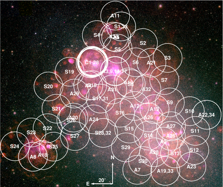
Figure 1: Colour image of the SMC from MCELS (e.g. Smith et al. 2000; Winkler et al. 2005) with H${\alpha}$/[S ii]/[O iii] in red, green, and blue. The overlaid circles indicate the distribution of XMM-Newton observations and have radii of 800″. Labels correspond to column 1 of Table LABEL:tab:observations.

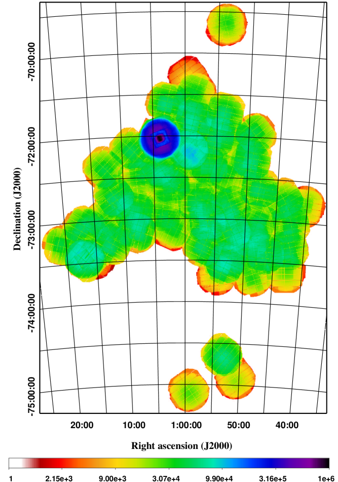
Figure 2: Combined vignetting-corrected EPIC exposure map of the SMC main field and additional outer fields, as used for the catalogue. The survey observation provide a homogeneous coverage in addition to the deep field around 1E0102.2-7219. EPIC-MOS1 and -MOS2 exposure is weighted by a factor of 0.4 relative to EPIC-pn to account for the lower effective area.

The XMM-Newton observatory (Jansen et al. 2001) comprises three X-ray telescopes (Aschenbach 2002) each equipped with a European Photon Imaging Camera (EPIC) at their focal planes, one of pn type (Strüder et al. 2001) and two of MOS type (Turner et al. 2001). This enables observations in the (0.2–12.0) keV band with an angular resolution of 5″–6″ (FWHM), which corresponds to a spatial resolution of $\sim$1.5 pc at the distance of the SMC.

In combination with archival observations, our large-programme SMC-survey provides complete coverage of the main body of the SMC (see Fig. 1). The survey was executed with EPIC in full-frame imaging mode, using the thin and medium filter for EPIC-pn and EPIC-MOS, respectively. Archival observations were partly performed in other modes.

To construct the XMM-Newton point-source catalogue for the SMC, we combined the data of the large-programme SMC survey (33 observations of 30 different fields, 1.1 Ms total exposure), with all publicly available archival data up to April 2010 (62 observations, 1.6 Ms exposure). Some 28 archival observations (850 ks in total) are calibration observations of the SNR 1E0102.2-7219. These calibration observations are performed every 6 months and constitute the deepest exposure XMM-Newton field in the SMC (see Fig. 2). All the observations form a continuous field, which we will refer to the main field (5.58 deg²). In addition, we included two observations of a field to the north and three fields to the south of the SMC main field (98 ks exposure in total). These are somewhat further away from the SMC bar and wing but contain SSSs found by ROSAT. The total area covered by the catalogue is 6.32 deg². A list of all exposures is given in Table LABEL:tab:observations. The table columns are described in detail in Sec. 4.1.

3 Creation of the source catalogue

To create a source catalogue for the SMC, we used a similar procedure as for the XMM-Newton Serendipitous Source Catalogue (2XMM, Watson et al. 2009). We built on similar studies of XMM-Newton observations of the Local-Group galaxies M 31 (Pietsch et al. 2005; Stiele et al. 2011) and M 33 (Pietsch et al. 2004; Misanovic et al. 2006). Compared to the standard XMM-Newton source catalogue, these catalogues have an improved positional accuracy by using boresight corrections from identified sources, plus a comprehensive source screening. The creation of our source catalogue is described in the following subsections. Further details are given in Appendix A.

3.1 Maximum-likelihood source detection

We first reprocessed all observations homogeneously with SAS 10.0.0 and created event lists using epchain or emchain, respectively. We used epreject to correct for artefacts in the EPIC-pn offset map. This avoids the detection of spurious apparently very-soft sources later on, but has the disadvantage of enhancing the effect of optical loading due to optically bright stars. Therefore we screened for bright stars as described in Sec. A.1.

To exclude time intervals of high background at the beginning or end of the satellite orbit, or during soft-proton flares, we applied a screening to remove time intervals with background rates in the (7.0$-$15.0) keV band, above 8 and 2.5 cts ks^-1 arcmin^-2 for EPIC-pn and EPIC-MOS, respectively. Since soft-proton flares affect all EPIC detectors, EPIC-pn and EPIC-MOS were allowed to veto each other, except for the observations 0503000301 and 0011450201, where the count rate in the high-energy band was significantly increased for EPIC-pn only. Therefore we used the EPIC-MOS data in these cases. For observations 0112780601, 0164560401, 0301170501 and 0135722201, the good time exposure was below 1 ks and we therefore rejected these observations. The resulting net exposures are given in Table LABEL:tab:observations. This good time selection procedure removed about 16% of exposures from the survey data, 22% from the calibration observations, 34% from other archival data and 10% of the outer fields. We discarded EPIC-pn events between 7.2 keV and 9.2 keV, since these are affected by background fluorescent emission lines, inhomogeneously distributed over the detector area (Freyberg et al. 2004). In the lowest energy band of EPIC-pn, we used an additional screening of recurrent hot pixels and for a few columns with increased noise where we rejected events below individual energy-offsets between 220 and 300 eV.

We produced images and exposure maps corrected for vignetting with an image pixel binning of $2\arcsec\times 2$″ in the five XMM-Newton standard energy bands: 1 $\rightarrow$ (0.2–0.5) keV, 2 $\rightarrow$ (0.5–1.0) keV, 3 $\rightarrow$ (1.0–2.0) keV, 4 $\rightarrow$ (2.0–4.5) keV, and 5 $\rightarrow$ (4.5–12.0) keV. We used single-pixel events for EPIC-pn in the (0.2–0.5) keV band, single- and double-pixel events for the other EPIC-pn bands, and single- to quadruple-pixel events for all EPIC-MOS bands. EPIC-MOS events were required to have FLAG=0. For EPIC-pn we selected (FLAG & 0xfa0000) = 0, which, as opposed to FLAG=0, allows events in pixels, when next to bad pixels or bad columns. This increases the sky coverage, but can also cause additional spurious detections, which need to be taken into consideration (see Sec. A.1).

We accomplished source detection on the images with the SAS task edetect_chain in all energy bands and instruments (up to $3\times 5$ images) simultaneously. We allowed two sources with overlapping point-spread function (PSF) to be fitted simultaneously. Possible source extension was investigated by using a $\beta$-model that approximates the brightness profile of galaxy clusters (Cavaliere & Fusco-Femiano 1976). This results in a source extent, with corresponding uncertainty, and a likelihood of source extent $ML_{\rm ext}$. A detailed description of the detection procedure can be found in Watson et al. (2009). As in the case of their catalogue, we accepted detections with $ML_{\rm det}=-\ln(P)\geq 6$, where $ML_{\rm det}$ is the detection likelihood, normalised to two degrees of freedom, and $P$ is the chance detection probability due to Poissonian background fluctuations.

3.2 Compilation of the point-source catalogue

Astrometric corrections of the positions of detections were applied, as described in Sec. A.2. We uniformly assume a systematic positional uncertainty of $\sigma_{\rm sys}=0.5$″ (Pietsch et al. 2005). The total positional uncertainty was estimated by $\sigma=(\sigma_{\rm sys}^{2}+\sigma_{\rm stat}^{2})^{1/2}$, where $\sigma_{\rm stat}$ is the statistical uncertainty, determined by emldetect. After a screening of the catalogue (see Sec. A.1), all 5236 non-spurious detections of point, or moderately extended, sources were auto-correlated to identify detections originating from the same source in a field which was observed several times. For the auto-correlation, we accepted correlations with a maximal angular separation of $d_{\rm sep}<7$″and $d_{\rm sep}<3(\sigma_{1}+\sigma_{2}$), where $\sigma_{1,2}$ is the total positional uncertainty of the two detections (see Watson et al. 2009). This resulted in 3053 unique X-ray sources. Master source positions and source extent were calculated from the error-weighted average of the individual detection values. Detection likelihoods were combined and renormalised for two degrees of freedom.

To investigate the spectral behaviour of all sources, we used hardness ratios $HR_{i}$ ($i=1,2,3,4$), defined by

$$HR_{i}=\frac{R_{i+1}-R_{i}}{R_{i+1}+R_{i}}$$

where $R_{i}$ is the count rate in energy band $i$ as defined in Sec.3.1. To increase statistics, we also calculated average HRs, combining all available instruments and observations. $HR_{i}$ is not given, if both rates $R_{i}$ and $R_{i+1}$ are null or if the 1$\sigma$ uncertainty of $\Delta HR_{i}$ covers the complete $HR$ interval from -1 to 1.

To convert an individual count rate $R_{i}$ of each energy band $i$ into an observation setup-independent, observed flux $F_{i}$, we calculated energy conversion factors (ECFs) $f_{i}=R_{i}/F_{i}$ as described in Sec. A.3. For the calculation, we assumed a universal spectrum for all sources, described by a power-law model with a photon index of $\Gamma=1.7$ and a photo-electric foreground absorption by the Galaxy of $N_{\rm H,Gal}=6\times 10^{20}$ cm^-2 (average for SMC main field in H i map of Dickey & Lockman 1990). For sources with several detections, we give the minimum, maximum and error-weighted average values for the flux.

In addition to the fluxes for each detection, we calculated flux upper limits $F_{\rm UL}$ for each observation and source, if the source was observed but not detected in the individual observation. As for the initial source detection, we used emldetect, with the same parameters as above, to fit sources, but kept the source positions fixed (xidfixed=yes) at the master positions and accepted all detection likelihoods in order to get an upper limit for the flux.

Following Primini et al. (1993), Misanovic et al. (2006) and Stiele et al. (2008), for the characterisation of the observed variability of sources covered by various XMM-Newton observations, we calculated the variability $V$ and its significance $S$ from

$$V=\frac{F_{\rm max}}{F_{\rm min}}\hskip 28.45274ptS=\frac{F_{\rm max}-F_{\rm min}}{\sqrt{\sigma_{\rm max}^{2}+\sigma_{\rm min}^{2}}}$$

where $F_{\rm max}$ and $\sigma_{\rm max}$ are the source flux and 1$\sigma$ uncertainty in the (0.2–4.5) keV band of the detection, for which $F-\sigma$ is maximal among all detections with a significance of $F>2\sigma$. In a similar way, $F_{\rm min}$ and $\sigma_{\rm min}$ were chosen from the detection, for which $F+\sigma$ is minimal among all detections, with $F>2\sigma$. In cases of $F<2\sigma$, we also considered $F_{\rm min}=3\sigma$ as a possible lower limit. Analogously, the minimum upper limit flux $F_{\rm UL}$ was selected from the observations, where the source was not detected. If the minimum $F_{\rm UL}$ was smaller than $F_{\rm min}$ defined above, we used it instead.

To investigate the flux variability within the individual observations, we used a Kolmogorow-Smirnow (KS) test to compare the photon arrival time distribution with the expected distribution from a constant source. This method is also applicable to sources with poor statistics, where background subtracted binned light curves cannot be obtained. A detailed description is given in Sec. A.4.

3.3 Estimation of sensitivity

To have an estimate of the completeness of the catalogue, we calculated sensitivity maps with esensmap for the individual energy bands and instruments, as well as for combinations of them, for each observation. Assuming Poisson statistics, detection limits for each position were calculated from the exposure and background maps. In the case of combined energy bands or instruments, the background images were added and the exposure maps were averaged, weighted by the expected count rate for the adopted universal spectrum of Sec. 3.2. The individual observations were combined, by selecting the observation with highest sensitivity at each position. We note that, depending on the individual source spectra, the detection limits deviate from this estimated value, but a detailed simulation of the detection limit goes beyond the scope of this study.

Figure 3: Histograms of the flux distribution of the individual detections of the XMM-Newton catalogue in various energy bands.

4 Catalogue description and characterisation

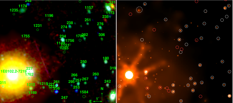
Figure 4: Left: XMM-Newton mosaic image of the deepest field in the SMC overplotted with the point-source catalogue. The image is background subtracted. Colours (red/green/blue) give logarithmically scaled intensities in the (0.2–1.0)/(1.0–2.0)/(2.0–4.5) keV bands. The brightest source is the oxygen-rich SNR 1E0102.2-7219. Right: Comparison with a deep Chandra image of the same region. The false-colour image gives logarithmically scaled intensities in the (0.2–10.0) keV band. XMM-Newton sources with low detection likelihood ($ML_{\rm det}<8$) are plotted in red, others in white.

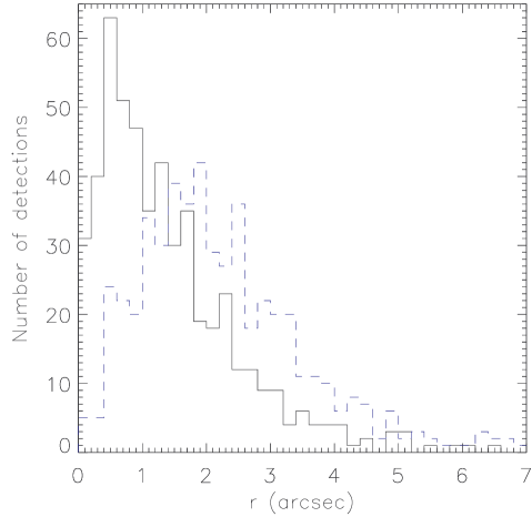
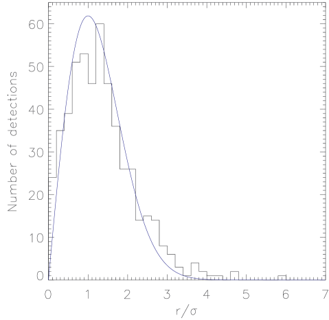
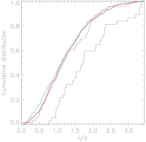
Figure 5: Left: Angular separation of X-ray and reference position of identified sources before (dashed blue line) and after (solid black line) boresight correction. Middle: Distribution of $r/\sigma$, compared with a Rayleigh distribution (blue line). Right: Cumulative distribution of angular separation between the XMM-Newton SMC catalogue and the Chandra catalogues of McGowan et al. (2008) in green, Laycock et al. (2010) in red, Nazé et al. (2003) in blue, and Evans et al. (2010) in orange. The cumulative Rayleigh distribution is shown by the black line.

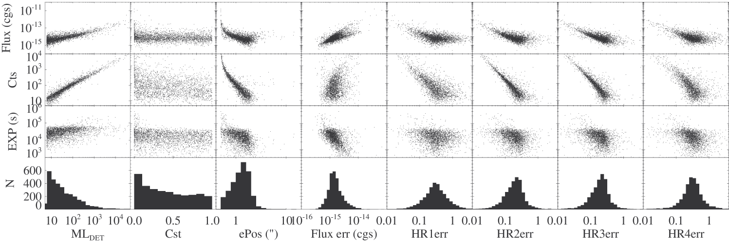
Figure 6: Dependence of various source parameters of the catalogue (maximum likelihood $ML_{\rm det}$, probability for time constancy $Cst$ and uncertainty of position $ePos$, flux in the (0.2–4.5) keV band and hardness ratios $HR$) on source flux, detected counts, and observation exposure. The lower panels show histograms of the distribution of these source parameters.

The catalogue contains a total of 3053 X-ray sources from a total of 5236 individual detections, either from the large-programme SMC survey between May 2009 and March 2010, or from re-analysed public archival observations between April 2000 and April 2010. For 927 sources, there were detections at multiple epochs, with some SMC fields observed up to 36 times.

4.1 Description

The parameters and instrumental setup of the individual observations are summarised in Table LABEL:tab:observations. The columns give the following parameters:
(1) = ID of the observation, where S,A,C, and O denote observations from the large-programme SMC survey, archival data, calibration observations and outer fields;
(2) = XMM-Newton Observation Id;
(3) = name of the observation target;
(4) = date of the beginning of the observation;
(5-6) = pointing direction;
(7-8) = boresight correction;
(9) = exposure Id;
(10) = start time of the exposure;
(11) = instrument filter;
(12) = instrument mode;
(13) = total exposure time;
(14) = exposure time after GTI screening, not considering the instrumental death time.

The source catalogue will be available at the Strasbourg Astronomical Data Center (CDS) and contains the following information:
(1) = unique source id (not continuous or ordered by coordinates);
(2) = XMM name;
(3) = number of detections of the source;
(4) = number of observations of the source;
(5) = combined maximum detection likelihood normalised for two degrees of freedom;
(6-7) = J2000 coordinates in degrees;
(8) = position uncertainty for 1$\sigma$ confidence (99.7% of all true sources positions are expected within a radius of $3.439\sigma$);
(9-22) = averaged fluxes and uncertainties in the five standard bands, in the combined band (0.2$-$12.0) keV and the XID band (0.2$-$4.5) keV, all in erg cm^-2 s^-1;
(23-24) = maximum of all detected fluxes of this source in the XID band in erg cm^-2 s^-1 and the corresponding uncertainties;
(25-26) = minimum or upper limit of all detected fluxes (as described in Sec. 3.2) in the XID band in erg cm^-2 s^-1;
(27-34) = hardness ratios between the standard bands and corresponding uncertainties;
(35-37) = averaged source extension, corresponding uncertainty and likelihood of extent;
(38) = KS-test probability, $Cst$, that the source was constant in all observations (the minimum value of all detections is taken, corresponding to the highest observed variability);
(39-40) = source variability $V$ between individual observations and corresponding significance $S$;
(41) = source classification;
(42) = name of identified sources.

4.2 Completeness, confusion, and spurious detections

In Fig. 3, the flux distribution of all individual source detections in several energy bands is presented. In the (0.2$-$4.5) keV and (0.2$-$12.0) keV band, we see a decreasing number density for fluxes lower than $10^{-14}$ erg cm^-2 s^-1 and $\sim$2$\times 10^{-14}$ erg cm^-2 s^-1. Thus we estimate the average detection threshold of our catalogue for sources in the SMC to be $\sim$5$\times 10^{33}$ erg s^-1 and $10^{34}$ erg s^-1, respectively. However, the inhomogeneous exposure time of the individual observations has to be taken into consideration.

In the field containing the calibration source 1E0102.2-7219, we can compare our catalogue with a deep XMM-Newton mosaic image (Fig. 4, left). Sources from our catalogue are overplotted with circles of 3.4$\sigma$ radii. Detections of 1E0102.2-7219 were screened, due to the high extent of this SNR. It is usually fitted with $\sim$5 sources. Other examples of identified sources (see Sec. 6) in the field are an active galactic nucleus (AGN) (№ 53), a HMXB (№ 227), a Wolf-Rayet star in the SMC (№ 1212), a Galactic star (№ 231), a SSS candidate (№ 235), and a cluster of galaxies (ClG, № 1174). Sources that are not clearly visible in the mosaic image can be due to them being weak and variable. Also, we stress that spurious detections in this field accumulate from 28 observations, because spurious detections are determined from the result of independent source detections performed on all 28 observations comprising the 1E0102.2-7219 calibration field. From the estimated number of spurious detections (see below) we expect $\sim$7 spurious sources in this image. A few additional sources appear in the deep mosaic image that are not listed in our catalogue, e.g. two sources left of № 251. The flux of these sources is below the detection limit of individual observations.

Since Chandra performs similar calibration observations of 1E0102.2-7219, we compare our results with a deep Chandra ACIS image (Fig. 4, right). It was created by merging 107 observations with the CIAO (version 4.3) task merge_all and adaptively smoothed. The exposure time is $\sim$920 ks decreasing with distance from 1E0102.2-7219, as the outer fields are not covered in all calibration observations. Our sources are overplotted with radii of 10″ in white and red for detection likelihoods of $ML_{\rm det}\geq 8$ and $ML_{\rm det}<8$, respectively. We see that source confusion is only relevant near the brightest sources (c.f. the surrounding of 1E0102.2-7219) and in some rare cases of close-by sources (e.g. source № 1157 might consist of two weak sources seen by Chandra). Source № 1174 is extended in the Chandra image, further supporting our ClG classification. We see that most sources with $ML_{\rm det}\geq 8$ are clearly visible in the Chandra image. № 235 is not found, due to the very soft spectrum and time variability. For sources with $ML_{\rm det}<8$, a corresponding source in the Chandra image is not always obvious.

To quantify spurious detections, we compared our catalogue with two deep Chandra SMC fields, where source lists are available (Laycock et al. 2010). All XMM-Newton sources, which were detected more than once or have a detection likelihood of $ML\gtrsim 8$, are also listed in the Chandra catalogue. Only 3 of 12 XMM-Newton sources with $ML_{\rm det}<8$ and one source with $ML_{\rm det}=8.2$ were not detected by Chandra. Some non-detections might be due to variability and the lower effective area of Chandra at the highest and lowest energies, but in general, as for the 2XMM catalogue, a fraction of detections with $ML_{\rm det}<8$ is expected to be spurious and should be regarded with care. In total, our catalogue contains 418 sources with $ML_{\rm det}<8$. From the former comparison, we roughly estimate around one hundred spurious detections among those, i.e. about one per observation.

4.3 Accuracy of source parameters

In Fig. 5 left, we show the angular separation of identified sources before and after the astrometric correction (Sec. A.2). The median of the total position uncertainty of all source positions is 1.3″. In Fig. 5 middle, the distribution of angular separation $r$ scaled by the total uncertainty $\sigma=(\sigma_{\rm sys}^{2}+\sigma_{\rm sta}^{2}+\sigma_{\rm ref}^{2})^{1/2}$ is shown, where $\sigma_{\rm ref}$ is the position uncertainty of the reference source. The distribution is similar to a Rayleigh distribution (blue line), which justifies our estimation of the systematic error of $\sigma_{\rm sys}=0.5$″. Since the same sample was used to determine the boresight corrections, some deviations from the Rayleigh distribution are expected. For example, for all observations containing only one identified source, the angular separation will be reduced to 0 due to the boresight shift.

To further test our positional accuracies with a statistically independent sample, we compared the final catalogue with available Chandra catalogues. In Sec. 5.3, we show that the correlation with these catalogues is close to a one-to-one, with a negligible number of chance coincidences. The catalogues are listed in Table 1. Sources, that have been used for boresight correction were excluded from this comparison. In Fig. 5 right, the cumulative distribution yields a good agreement with the catalogues of McGowan et al. (2008), Laycock et al. (2010), and Evans et al. (2010) with KS-test statistics of 22%, 47%, and 77%, respectively. Only for sources of Nazé et al. (2003), an unexpected distribution of angular separations is found, with a KS-test statistic of 0.097%. In a further investigation, we found a systematic offset of the Chandra positions relative to the XMM-Newton positions by $\sim$1.7″. The offset is also evident when we compare the Chandra coordinates to the Tycho-2 position of HD 5980 and the Magellanic Clouds Photometric Survey catalogue (MCPS, Zaritsky et al. 2002) positions of SXP 152 and SXP 304. Therefore, we conclude that the coordinates of these Chandra sources are wrong by a systematic offset.

An overview of the distribution of source parameter uncertainties and probabilities for existence $ML_{\rm det}$ and constancy $Cst$, as well as their dependence on observational parameters, is shown in Fig. 6. The number of counts is the main quantity on which they depend. For 2378 and 2635 sources, the detection maximum likelihood is $ML_{\rm det}>10$ and $>$8, respectively. The relative uncertainties of fluxes in the (0.2$-$4.5) keV band have a median of 22%. For the uncertainties of the hardness ratios 1 to 4, we obtain the medians of 0.30, 0.20, 0.20, and 0.31, respectively.

5 Cross-correlation with other catalogues

Table 1: Reference catalogues used for cross-correlation.

Catalogue	Type	Reference	$\sigma_{\rm ref}(\arcsec)$	$N_{\rm cat}$	$N_{\rm ref}$	$N_{\rm XMM}$	$C_{\rm ref}$	$C_{\rm XMM}$
Einstein	X-ray	1	40	50	48	154	45.1$\pm$1.6	131$\pm$13
Einstein	X-ray	1	40	50	26	27	6.1$\pm$2.1	6.5$\pm$2.4
ROSAT PSPC	X-ray	2	10	353	282	353	40.9$\pm$4.5	55.5$\pm$7.4
ROSAT PSPC	X-ray	2	10	353	236	264	15.3$\pm$4.0	17.9$\pm$4.6
ROSAT HRI	X-ray	3	2.6	109	76	78	2.4$\pm$1.8	2.4$\pm$1.8
ASCA	X-ray	4	18.6	83	69	111	33.1$\pm$4.2	42.5$\pm$6.1
Chandra Wing Survey	X-ray	5	1.02	393	242	240	2.3$\pm$1.6	2.3$\pm$1.5
Chandra deep fields	X-ray	6	0.66	394	85	85	1.8$\pm$1.4	1.7$\pm$1.3
Chandra NGC 346	X-ray	7	0.30	75	41	41	0.58$\pm$0.64	0.63$\pm$0.70
CSC (release 1.1)	X-ray	8	1.30	496	368	373	8.2$\pm$2.4	9.4$\pm$3.4
MCPS	opt.	9	0.3	2872224	10484	2604	10082$\pm$75	2431$\pm$21
Tycho-2	opt.	10	0.078	321	41	41	1.5$\pm$1.1	1.5$\pm$1.2
GSC (version 2.3.2)	opt.	11	0.43	855524	3476	2099	3045$\pm$42	1752$\pm$20
2MASS	NIR	12	0.15	159491	923	743	565$\pm$27	427$\pm$17
2MASX	NIR	12	4.4	223	26	26	8.5$\pm$2.4	9.0$\pm$2.7
DENIS MC	NIR	13	0.47	94357	609	540	364$\pm$19	303$\pm$15
DENIS (3rd release)	NIR	14	0.3	438517	2058	1043	1477$\pm$55	737$\pm$18
IRSF Sirius	NIR	15	0.1	1855973	8426	2407	6500$\pm$110	1914$\pm$22
S3MC	IR	16	1, 3, 6	400735	3403	1711	2193$\pm$40	1108$\pm$17
ATCA RCS	radio	17,18	1.0	301	31	31	1.6$\pm$1.2	1.6$\pm$1.2
SUMSS (version 2.1)	radio	19,20	3.0	246	46	47	5.3$\pm$2.2	5.5$\pm$2.3
MA93	H${\alpha}$	21	2.0	1805	63	62	18.6$\pm$3.0	18.2$\pm$3.4
Murphy2000	H${\alpha}$, [O iii]	22	3.5, 4.4	286	12	12	7.4$\pm$2.6	7.3$\pm$2.7
2dF SMC	stellar classification	23	0.5	2874	31	31	8.8$\pm$3.4	8.7$\pm$3.4
6dF GS	galaxy redshifts	24	1.0	16	6	6	0.04$\pm$0.20	0.04$\pm$0.20
Kozlowski2009	AGN candidates	25	1.0	655	146	148	3.9$\pm$2.2	3.8$\pm$2.1
Bica2008	star cluster	26	26.6	409	41	45	29.0$\pm$6.1	32.1$\pm$6.6
Bonatto2010	star cluster	27	33.7	75	11	14	7.8$\pm$2.9	9.4$\pm$3.2

(1) Wang & Wu (1992); (2) Haberl et al. (2000); (3) Sasaki et al. (2000); (4) Yokogawa et al. (2003); (5) McGowan et al. (2008); (6) Laycock et al. (2010); (7) Nazé et al. (2003); (8) Evans et al. (2010); (9) Zaritsky et al. (2002); (10) Høg et al. (2000); (11) Lasker et al. (2008); (12) Skrutskie et al. (2006); (13) Cioni et al. (2000); (14) DENIS Consortium (2005); (15) Kato et al. (2007); (16) Bolatto et al. (2007); (17) Filipović et al. (2002); (18) Payne et al. (2004); (19) Bock et al. (1999); (20) Mauch et al. (2003); (21) Meyssonnier & Azzopardi (1993); (22) Murphy & Bessell (2000); (23) Evans et al. (2004); (24) Jones et al. (2009); (25) Kozłowski & Kochanek (2009); (26) Table 3 of Bica et al. (2008); (27) Bonatto & Bica (2010).

To classify and identify individual sources, we cross-correlated the boresight-corrected positions of our XMM-Newton SMC point-source catalogue with publicly available catalogues. The correlations with X-ray catalogues from previous studies allows us to study the evolution of X-ray sources with time. Other wavelength catalogues add ancillary information, enabling a multi-wavelength analysis. The catalogues used are listed in Table 1 together with statistical properties of the correlations.

5.1 Selection of counterparts

The uncertainties of the XMM-Newton source coordinates are radially symmetric, as is the case for most of the other catalogues. For some catalogues with higher positional accuracy, elliptical errors are given (e.g. 2MASS). Since the XMM-Newton positional uncertainty is dominant, for simplicity we assumed radial symmetric uncertainties for all catalogues and used the semi-major axis as the radius if elliptical errors are given. When confidence levels for the positional uncertainty are given, we recalculated the positional uncertainty of the reference catalogue $\sigma_{\rm ref}$ for 1$\sigma$ confidence. In some cases, the uncertainties had to be estimated. Following Watson et al. (2009), we consider all correlations having an angular separation of $d\leq 3.439\times(\sigma_{\rm sys}^{2}+\sigma_{\rm sta}^{2}+\sigma_{\rm ref}^{2})^{1/2}$ as counterpart candidates. This corresponds to a 3$\sigma$ (99.73%) completeness when we assume a Rayleigh distribution. The resulting number of matched XMM-Newton and reference sources, $N_{\rm XMM}$ and $N_{\rm ref}$, is given in Table 1.

5.2 Estimation of chance correlations

Depending on the source density and positional uncertainty, the number of chance coincidences, $C_{\rm XMM}$ and $C_{\rm ref}$, has to be considered. These were estimated by shifting our catalogue in right ascension and declination by multiples of the maximal possible correlation distance between two sources in both catalogues and using the same correlation criterion as above. We performed several of these correlation runs to investigate variations of chance coincidences.

In Fig. 7 we give examples of the dependence of the number of chance-correlations $C_{\rm XMM}$ on the shifting distance. In the case of the 2MASS catalogue, we see only a small systematic decrease with increasing offset that is negligible, compared to the standard deviations. If the coordinate shift becomes too large, a variable source-density can affect the number of correlations. This is the case for catalogues with inhomogeneously distributed sources, e.g. due to the SMC morphology or a limited SMC-specific field of the catalogue. When investigating the dependence of the number of correlations on shifting distance, we found no significant variations on a scale of a few shifts, with the exception of the correlation with the Einstein catalogue. The variations found for the Einstein catalogue are caused by relatively large positional uncertainties that require a large coordinate shift.

In order to estimate the variation of the number of chance coincidences, we used 24 shifted correlations of a $5\times 5$ grid. All these samples result from coordinate shifts between $d_{\rm max}$ and $\sqrt{8}d_{\rm max}$. The comparison with the Einstein catalogue was done with a $3\times 3$ grid. The averaged numbers of chance coincidences for our catalogue $C_{\rm XMM}$ and the reference catalogue $C_{\rm ref}$ are given in Table 1. Their uncertainties are estimated using their standard deviation. By comparing these values with the number of real correlations, we can estimate the contribution of chance coincidences. In general, we find that correlations with Chandra X-ray sources, radio sources and IR-selected AGN candidates are quite robust, whereas correlations with optical to infrared catalogues are dominated by the contribution of chance coincidences. The number of multiple coincidences can be estimated by comparing the number of matched sources in our catalogue $N_{\rm XMM}$ to the number of matched sources of the reference catalogues $N_{\rm ref}$. Correlations with radio and Chandra X-ray catalogues are close to a one-to-one correlation, whereas for dense optical catalogues four times more reference sources are found than X-ray sources. In the case of the MCPS, 74% of the matched XMM-Newton sources have more than one, and 53% have more than two counterpart candidates.

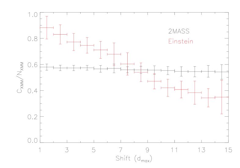
Figure 7: Examples for the chance-correlation dependence on offset. The data points are binned in units of maximal correlation distance ($d_{\rm max}$). For each bin, the average of chance-correlation $C_{\rm XMM}$ is given, normalised to the number of correlations $N_{\rm XMM}$ with unshifted coordinates. The error bars give the standard deviation for each bin.

5.3 Correlation with other X-ray catalogues

We correlated our catalogue with X-ray catalogues from previous studies. From earlier epochs we used X-ray sources detected with the Einstein observatory between 1979 and 1980 (Wang & Wu 1992), ROSAT sources from Haberl et al. (2000) and Sasaki et al. (2000) detected between 1990 and 1998, and ASCA sources from observations between 1993 and 2000 (Yokogawa et al. 2003). Due to the aforementioned high positional uncertainties of the Einstein catalogue and the higher sensitivity of XMM-Newton, the correlation is dominated by chance coincidences, so most Einstein sources cannot be assigned uniquely to an XMM-Newton source. A more unambiguous correlation can be achieved if a set of the brightest XMM-Newton sources, with fluxes $>5\times 10^{-14}$ erg cm^-2 s^-1, is used. Similarly, we find an improvement for the correlation with the ROSAT PSPC catalogue, if we impose a limit of sources with fluxes $>10^{-14}$ erg cm^-2 s^-1. These results are also listed in Table 1. By comparing the catalogues and mosaic images, we found about 30 ROSAT sources, without a corresponding XMM-Newton source. Eight can be associated with variable sources (HMXB or SSS), while others are faint and might be spurious or affected by confusion of multiple sources or diffuse emission.

Based on Chandra observations since 1999, there are several catalogues from the same era as the XMM-Newton data but covering only some part of the SMC main field: fields in the SMC wing (McGowan et al. 2008), deep fields in the SMC bar (Laycock et al. 2010), and sources around NGC 346 (Nazé et al. 2003). Additional sources were taken from the Chandra Source Catalogue (CSC, Evans et al. 2010). In general for comparable exposures, these catalogues offer more precise positions but have fewer counts per detection compared to XMM-Newton detections. The correlation between the XMM-Newton and Chandra sources is close to a one-to-one correlation with less then 2% of chance coincidences.

5.4 Correlation with catalogues at other wavelength

To identify the optical counterparts we used the Magellanic Clouds Photometric Survey catalogue (MCPS, Zaritsky et al. 2002), providing stellar photometry in $U$, $B$, $V$ and $I$ down to magnitudes of $\sim$20–22 mag. Due to the high source density compared to the XMM-Newton resolution, the cross correlation is dominated by chance coincidences. To identify bright foreground stars, which are not listed in the MCPS, we used the Tycho-2 catalogue (Høg et al. 2000), which has a completeness of 99% for $V\sim 11.0$ mag and provides proper motions and $B_{\rm T}$ and $V_{\rm T}$ magnitudes. Since the MCPS does not cover all parts of the XMM-Newton field and some stars around $V\sim 12$ mag are too faint for the Tycho-2 catalogue but too bright for the MCPS, we used the Guide Star Catalogue (GSC, Lasker et al. 2008) in these cases, which gives $B_{\rm J}$ and $R_{\rm F}$ magnitudes down to $\sim$21 mag. For 129 X-ray sources which do not have a counterpart in either of the MCPS and Tycho-2 catalogues, we found a possible counterpart in the GSC.

Near-infrared sources in $J$, $H$, and $K_{\rm S}$ were taken from the Two Micron All Sky Survey (2MASS, Skrutskie et al. 2006), the Deep Near Infrared Survey (DENIS, Cioni et al. 2000; DENIS Consortium 2005), and the InfraRed Survey Facility (IRSF) Sirius catalogue of Kato et al. (2007). Since these catalogues contain measurements from different epochs, they allow us to estimate the NIR variability of X-ray sources, which is especially interesting for HMXBs.

Infrared fluxes at 3.6, 4.5, 5.8, 8.0, 24, and 70 $\mu$m are taken from the Spitzer Survey of the SMC (S³MC, Bolatto et al. 2007). Radio sources were taken from the ATCA radio-continuum study (Payne et al. 2004; Filipović et al. 2002), with ATCA radio point-source flux densities at 1.42, 2.37, 4.80, and 8.64 GHz, and from the Sydney University Molonglo Sky Survey at 843 MHz (SUMSS, Mauch et al. 2003). These correlations enable a classification of background sources.

Furthermore, we compared our sources with some individual catalogues providing emission-line sources (Meyssonnier & Azzopardi 1993; Murphy & Bessell 2000), stellar classification (Evans et al. 2004), galaxies confirmed by redshift measurements (Jones et al. 2009), and IR selected AGN candidates (Kozłowski & Kochanek 2009). For the correlation with the catalogues of star clusters (Bica et al. 2008; Bonatto & Bica 2010), we used the semi-major axis of the cluster extent as a $3\sigma$ uncertainty for the reference position.

6 Source identification and classification

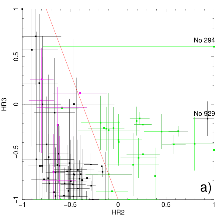
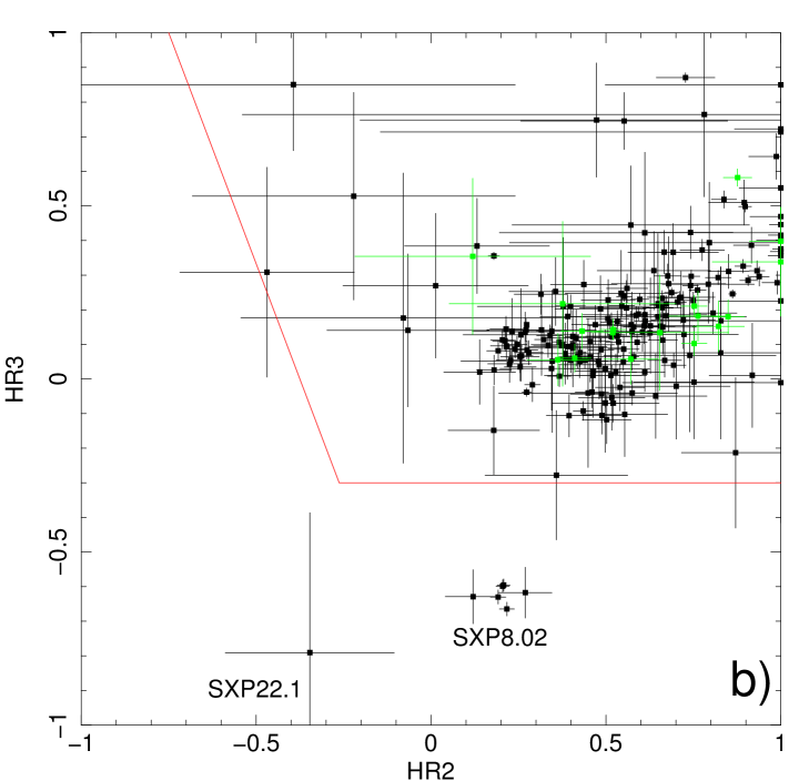
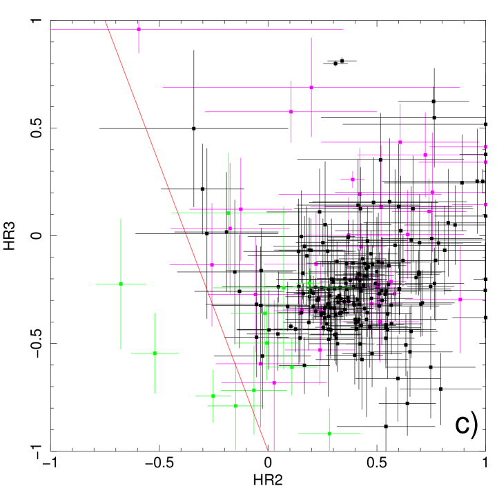
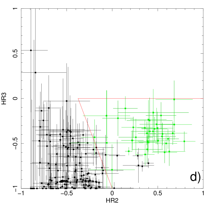
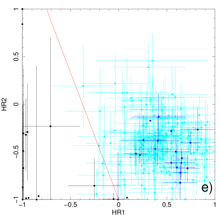
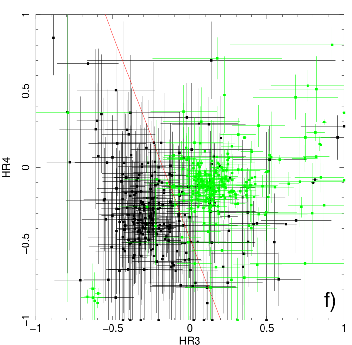
Figure 8: Hardness-ratio diagrams for XMM-Newton detections of various source classes. Red lines show HR-selection cuts as used for our source classification. ^(a) Detections with optical counterparts in the Tycho-2 catalogue. Galactic stars are shown in black and magenta, SMC-stars in green. Details are given in Sec.  6.1. ^(b) Detections of known pulsars (black) and identified HMXBs (green). See Sec.  6.3. ^(c) Detections of spectroscopically confirmed AGN (black), radio background sources (magenta) and galaxies (green). See Sec. 6.4. ^(d) Detections of sources, screened due to their extent. SNRs are shown in black, other sources (likely galaxy clusters) in green. See Sec. 6.6. ^(e) Comparison of detected SSSs in the SMC and LMC (black) with identified (blue) and classified (cyan) stars in the $HR_{1}$-$HR_{2}$-plane. See Sec. 6.2. ^(f) Comparison of AGN and radio sources from c) (black) with pulsars and HMXBs from b) (green) in the $HR_{3}$-$HR_{4}$-plane. See Sec.  6.3.

Table 2: Spectral classification of the X-ray source sample.

Spectrum	Classified	Selection criteria
super soft	18	($8HR_{1}+3HR_{2}<-3$ or ($HR_{1}<-0.75$ && $HR_{2}$ not def.))
		&& $F_{1}>3\Delta F_{1}$ && $F_{3}<3\Delta F_{3}$ && $F_{4}<3\Delta F_{4}$ && $F_{5}<3\Delta F_{5}$
soft	298	$8HR_{2}+3HR_{3}<-3$ or ($HR_{2}<-0.75$ && $HR_{3}$ not def.)
hard	2711	($8HR_{2}+3HR_{3}>-3$ or ($HR_{2}>0\&\&HR_{3}$ not def.)) && not super soft
ultra hard	945	$8HR_{3}+3HR_{4}>-1.4$ or ($HR_{3}>0.2\&\&HR_{4}$ not def.) && not soft && not super soft
unclass.	8	–

Table 3: Source classification criteria.

Class	Classification criteria	Identified	Classified
ClG	hard && $HR_{3}$$<$0 && Ext$>$$\Delta$Ext && $ML_{\rm Ext}$$>$10	12	13
SSS	super soft && no opt. loading && $ML_{\rm det}>10$ && ($N_{\rm det}>1$ or ($ML_{\rm pn}>4$ && $(ML_{\rm m1}>2$ or $ML_{\rm m2}>2)))$	4	8
fg-star	soft && $\log{(f_{X}/f_{o})}<-1$ && ($B-V>1.2$ or $(B-V>0.3\&\&V>17))$	34	128
AGN	hard && appropriate radio (r), infrared (i), X-ray (x) or optical (o) counterpart	72	2106
HMXB	ultra hard && $13.5<V<17.0$ && $-0.5<B-V<0.5$ && $-1.5<U-B<-0.2$ && no AGN id	49	45

Besides X-ray sources within the SMC, the observed field contains Galactic X-ray sources and background objects behind the SMC. To distinguish between these, we identified and classified individual sources. For identification, we searched the literature as described below and selected secure cases only.

To classify the unidentified sources, we developed an empirical approach following Pietsch et al. (2004). We derived classification criteria obtained from the parameters of individual detections of identified sources as seen with XMM-Newton in our processing. Individual source detections were used, instead of averaged source values, to increase the statistics and account for spectral variability, since $\sim$70% of our sources were only detected once. Classifications are marked by angle brackets ($<$class$>$). We note that classes give likely origins for the X-ray emission, but have to be regarded with care.

First, we distinguished between point sources and sources fitted with small, but significant, extent. Most of these sources were classified as clusters of galaxies ($<$ClG$>$, see Sec. 6.6 and Table 6). Sources with extent too large to be modelled properly by emldetect as one single source (e.g. SNRs with substructure), were flagged beforehand and were not included in the final catalogue. An overview of these sources can be found in Haberl et al. (2012a).

The remaining point sources were classified using X-ray hardness ratios and multi-wavelength properties. Using the selection criteria given in Table 2, we divided our sample into super-soft, soft, hard, and ultra-hard sources. We selected super-soft X-ray sources first, which are classified only if detector noise is an unlikely alternative explanation. Soft X-ray sources are classified as foreground stars if they have an appropriately bright optical counterpart that is unlikely to be within the SMC on the basis of its brightness and colours. Also, depending on the counterpart, hard X-ray sources were classified as either AGN or HMXB. An overview of our classification criteria and results is presented in Table 3. The hardness ratios of identified sources are compared in Fig. 8. By comparing our classification result with the source classification of Haberl et al. (2000) and McGowan et al. (2008), we found a good agreement. Details for each source class are given in the following.

6.1 X-rays from non-degenerate stars

Shocks in the wind of OB stars, coronal activity from F to M stars, accretion processes in T Tau stars and interaction of close-binary stars can cause X-ray emission from non-degenerate stars (for a review see Güdel & Nazé 2009). Because such stars are weak X-ray sources, most of them in the SMC are below the sensitivity limit of our survey. Galactic stars are foreground sources, expected to be homogeneously distributed in the XMM-Newton SMC field and due to their high galactic latitude ($b\sim-44.5$°), the sample is expected to be dominated by late-type stars. Compared to distant Local-Group galaxies, the identification of Galactic stars as X-ray sources in front of the SMC is challenging, because luminous SMC stars and faint Galactic stars can have a similar brightness, so are hard to differentiate.

6.1.1 Identification of Galactic stars

To identify the brightest ($V<11$ mag) foreground stars, we used our correlation with the Tycho-2 catalogue, where we expect one or two chance coincidences. 40 individual X-ray sources with a Tycho-2 counterpart resulting in 84 XMM-Newton detections with determined $HR_{2}$ and $HR_{3}$ are plotted in Fig. 8 a. For three further detections of these sources and one additional X-ray source $HR_{3}$ is undefined and $HR_{2}\leq-0.9$.

There are 33 Tycho-2 sources with significant ($>$3$\sigma$) proper motions that are all $>$8 mas yr^-1. These are obviously foreground stars. Two more counterparts are stars with a late-type main-sequence classification (Wright et al. 2003). X-ray detections of these 35 confirmed foreground stars are plotted in black in Fig. 8a. Twenty-five detections of three Tycho-2 sources, correlating with SMC-stars (see Sec. 6.1.3), are plotted in green. The remaining three matches (№ 140, 2008, and 2158) were classified as candidates for Galactic stars ($<$fg-star$>$, plotted in magenta). Source № 929 shows harder X-ray colours than the remaining foreground stars and is therefore not classified. The optical and X-ray emission might correlate by chance, but also a foreground cataclysmic variable (CV) is possible.

6.1.2 Classification of Galactic stars

To classify an X-ray source as a foreground star candidate ($<$fg-star$>$), we require four criteria:

(i) Using the Tycho-2 set of 35 confirmed foreground stars, we defined a cut (red line in Fig. 8a) for the X-ray colour selection of fg-star candidates ($<$fg-star$>$), which separates them from hard X-ray sources, such as AGN and HMXBs (see below and cf. Fig. 8b and c). For faint soft sources with a low $HR_{2}$ value, the count rate $R_{4}$ will not be well determined, leading to an unconstrained $HR_{3}$. Our selection allows a less precise determined $HR_{3}$ for sources with lower $HR_{2}$. From similar source samples, a correlation between X-ray plasma temperature and spectral type is not found (Wright et al. 2010). Therefore, we do not expect a bias in our selection method, although the selection criteria on X-ray hardness ratios are defined using the Tycho-2 catalogue that contains only the brightest stars in the $B$ and $V$ bands. We find 258 unidentified soft X-ray sources in our catalogue.

(ii) For stars with fainter optical magnitudes, it becomes more complicated to discriminate between stars in the Galaxy and the SMC. In addition to soft X-ray colours, the source must have a sufficiently bright optical counterpart. Following Maccacaro et al. (1988), we calculated

$$\log{(f_{X}/f_{o})}=\log{(F_{(0.2-4.5){\rm keV}})}+\frac{V}{2.5}+5.37$$

for the MCPS correlations and

$$\log{(f_{X}/f_{o})}=\log{(F_{(0.2-4.5){\rm keV}})}+\frac{R+B}{2\times 2.5}+5.37$$

for GSC correlations, where the X-ray flux is in units of erg cm^-2 s^-1. We classified sources as foreground-star candidates ($<$fg-star$>$) only, if they have an optical counterpart with $\log{(f_{X}/f_{o})}<-1$. Of the 258 sources, 197 have a sufficiently bright optical counterpart in the MCPS. The dependence of X-ray flux on optical $V$ magnitude is plotted in Fig. 9. For foreground stars we expect to find an optical counterpart with the given sensitivity of the MCPS.

(iii) Since optical counterparts are still outnumbered by chance correlations with stars of the SMC, we used a colour selection to exclude most of them. In Fig. 10, we show the colour-magnitude and colour-colour diagram of all optical counterpart candidates of X-ray sources with measured $U$, $V$, and $B$ magnitudes in the MCPS (black points). To avoid main-sequence and horizontal-branch stars of the SMC, we only selected optical counterparts to the right of the blue dashed line, which have $V<17$ mag and $B-V>0.3$ mag or $B-V>1.2$ mag without any magnitude selection. This reduces the foreground star sample to 107 sources.

For source № 548, we found a Tycho-2 colour of $B-V=-0.38$. However, this source is identified with the Galactic star Dachs SMC 3-2 and other catalogues give $B-V=0.70$ (e.g. Massey 2002). The Tycho-2 colour is regarded as an outlier and corrected with the magnitudes of Massey (2002) for Fig. 10.

(iv) To avoid possibly erroneous correlations, we did not classify X-ray sources with a positional uncertainty of more than 3″ (4 sources).

This allowed us to classify 103 candidates for foreground stars. To estimate the number of chance coincidences, we shifted the coordinates of one catalogue. For 26$\pm$5 of the 249 unidentified soft X-ray sources with $ePos<3\arcsec$, we find at least one counterpart candidate compatible with the selection criteria for stars by chance. When we take into account that some true correlations cause chance correlation when their coordinates are shifted, we estimate that $\sim$$(16.1\pm 3.6)\%$ of the classified foreground stars are chance coincidences. In addition, using the GSC in cases where the X-ray source did not have a counterpart in the Tycho-2 or MCPS catalogues, we classified 17 X-ray sources as foreground stars.

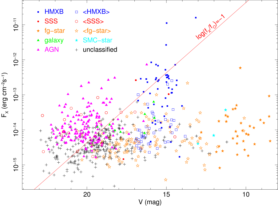
Figure 9: Optical $V$-band magnitude vs. the detected X-ray flux in the (0.2–4.5) keV band for various source classes. For foreground stars, the brightest correlated source is plotted. For HMXB we selected the counterparts as in Sec. 6.3.2. For all other sources, the nearest optical counterpart is plotted.

However, the X-ray emission of stars can become harder during flares (e.g. Güdel et al. 2004), so that our hardness-ratio selection criteria can be violated. Similarly, as the X-ray flux increases the $f_{X}/f_{o}$ criteria might also be violated. This causes some overlap with AGN in hardness ratios and $f_{X}/f_{o}$. To investigate this possibility, we searched for sources with short-term variability $Cst<0.5\%$ and $f_{X}/f_{o}>0$. To exclude HMXBs and the bulk of AGNs we also required $HR_{2}<0.2$ and $HR_{3}<-0.3$. We selected five additional sources (№ 146, 1998, 2041, 2740, and 3059) as candidates ($<$fg-star$>$).

For 61 stars, which have a 2MASS counterpart in the MCPS catalogue, we derived a spectral classification from the $J-K$ colour (see Bonfini et al. 2009). The resulting distribution of the spectral types is shown in Fig.11 and follows the expected distribution, peaking around early M stars.

6.1.3 Stars within the SMC

In some extreme cases, X-ray emission from early-type stars within the SMC can be observed with XMM-Newton, e.g. from stellar-wind interaction of a Wolf-Rayet star in a binary system with an OB star. Guerrero & Chu (2008) found X-ray emission from SMC-WR5, SMC-WR6, and SMC-WR7 (Massey et al. 2003), which are the sources № 150, 237, and 1212 in our catalogue (cyan stars in Fig. 9 and Fig. 10, left). № 1212 is visible in Fig. 4.

For completeness, we note that source № 145 is close to SMC-WR3, but due to a separation of 3.29″ (2.73$\sigma$), this correlation is doubtful. Also, sources № 294, 1031, and 2963 formally correlate with the SMC stars AzV 369 (4.6″, 3.1$\sigma$), AzV 222 (4.1″, 2.8$\sigma$), and 2dFS 3274 (1.8″, 1.0$\sigma$).

In the centre of the star cluster NGC 346 we see an unresolved convolution of X-ray bright stars (see Nazé et al. 2002, 2004), which is source № 535 in our catalogue. Source № 2706 has similar X-ray colours and correlates with the star cluster Lindsay 66. Also № 294 can be associated with the star cluster Bruck 125. From our correlation with the star cluster catalogue of Bica et al. (2008), we expect around 13$\pm$7 X-ray sources to be correlated with star clusters. About half of these sources can be explained by HMXBs, which might have formed in these clusters (Coe 2005).

6.2 Super-soft X-ray sources

SSSs are a phenomenological class of X-ray sources, defined by a very soft thermal X-ray spectrum and with no emission above 1 keV. Luminous SSSs are associated with CVs, planetary nebulae, symbiotic stars, and post-outburst optical novae. The general scenario is steady thermonuclear burning on the surface of an accreting white dwarf (Nomoto et al. 2007). Less luminous SSSs can be observed in some CVs, cooling neutron stars and PG 1159 stars. For a review, see Kahabka (2006).

Table 4: Faint SSS candidates in the SMC.

No.	RA	Dec	ePos	$HR_{1}$	$HR_{2}$	$F$	$ML_{\rm det}$	$ML_{\rm pn}$	$ML_{\rm m1}$	$ML_{\rm m2}$	Comment
235	01 01 47.58	-71 55 50.7	0.85	-0.3$\pm$0.1	-0.8$\pm$0.1	6.0$\pm$0.6	146.5	54.7	33.2	4.2	WD/Be?
1198	01 01 24.19	-72 00 37.9	1.82	-0.4$\pm$0.2	-1.0$\pm$0.5	2.5$\pm$0.7	16.2	9.4	6.2	2.8
1531	00 39 45.58	-72 47 01.4	1.58	-1.0$\pm$0.1	0.8$\pm$0.4	1.8$\pm$0.4	28.6	10.7	7.8	12.2	star?
1549	00 38 58.74	-72 55 10.4	1.68	-1.0$\pm$0.2	–	3.6$\pm$0.9	18.3	13.6	4.5	2.9	star?
2132	00 57 45.29	-71 45 59.7	0.93	-0.4$\pm$0.1	-0.5$\pm$0.2	4.1$\pm$0.5	121.1	85.4	20.4	18.8
2178	00 55 37.71	-72 03 14.0	0.74	-0.9$\pm$0.0	0.2$\pm$0.4	6.7$\pm$0.5	391.5	282.6	54.5	58.7
2218	00 55 08.45	-71 58 26.7	1.38	-0.2$\pm$0.2	-0.9$\pm$0.4	1.3$\pm$0.3	14.0	13.0	3.2	0.9	WD/Be?, star?
3235	00 55 03.65	-73 38 04.1	0.64	-0.9$\pm$0.0	0.2$\pm$0.2	13.6$\pm$0.8	787.0	649.0	48.1	96.2

6.2.1 Identification of super-soft X-ray sources

Two bright SSSs in the SMC, the planetary nebula SMP SMC 22 (№ 686) and the symbiotic nova SMC3 (№ 616), were observed during our survey (Mereghetti et al. 2010; Sturm et al. 2011b). In addition, Mereghetti et al. (2010) confirmed SMP SMC 25 as a faint SSS in the survey data (№ 1858), that was discovered with ROSAT by Kahabka et al. (1999). Other SSSs known from ROSAT (RX J0059.1-7505, RX J0059.4-7118, RX J0050.5-7455), were previously observed with XMM-Newton (Kahabka & Haberl 2006). The first source is the symbiotic star LIN 358 (№ 1263), the second was suggested to be a close binary or isolated neutron star (№ 324), for the third source Kahabka & Haberl (2006) give an upper limit. In our survey analysis, this latter source is detected (№ 1384), but is very probably associated with the Galactic star TYC 9141-7087-1 and affected by optical loading. Other ROSAT sources from Kahabka & Pietsch (1996) are the transient SSS RX J0058.6-7146 and the candidate SSS RX J0103.8-7254. For neither source can we find a detection in our catalogue. The position of the variable SSS 1E0035.4-7230 is not covered by any XMM-Newton observation yet. Source № 235 was found as a new faint SSS candidate (see Sec. 6.2.2) and is proposed to be a binary system consisting of a white dwarf and a Be star (Sturm et al. 2012). The position of the super-soft transient MAXI J0158-744 (Li et al. 2012) was not covered with XMM-Newton. New luminous SSS transients were not found during the XMM-Newton SMC survey.

6.2.2 Search for faint SSS candidates

The XMM-Newton survey enables a search for faint SSSs. Analogously to our division into soft and hard X-ray sources in Sec. 6.1, we separate super-soft from soft X-ray sources in the $HR_{1}$-$HR_{2}$-plane, as shown in Fig. 8e. Detections of identified SSSs from Sec. 6.2.1, are plotted in black. To increase the reference sample, we also used detections of identified SSSs in the LMC (see Kahabka et al. 2008, and references therein), from an identical data processing method as used for the SMC data. In general, $HR_{1}$ is negative for SSSs and depends strongly on photo-electric absorption. $HR_{2}$ is expected to be close to -1, but due to low count rates in the energy bands 2 and 3, $HR_{2}$ is only poorly determined for weak SSSs. We also demand no significant ($<$3$\sigma$) emission in the energy bands 3–5, but significant emission in the energy band 1, to designate the spectrum as super soft. The two LMC SSSs outside our selection area are CAL 87 and RX J0507.1-6743, which are both affected by high absorption (Kahabka et al. 2008) causing a $HR_{1}$ of $0.087\pm 0.003$ and $0.22\pm 0.08$, respectively. Identified Tycho-2 stars (Sec. 6.1), which are not affected by optical loading, are plotted in blue. In cyan, we show all sources, which fulfil our selection criteria for candidate foreground stars, have a detection likelihood of $ML_{\rm det}>10$ and are not affected by optical loading. Three of these sources fulfil the selection criteria of both SSS and stars. Here a X-ray spectral analysis is necessary to discriminate between them.

Unfortunately, optical loading and detector noise cause spurious detections with characteristics similar to SSS. EPIC-MOS is less sensitive below 500 eV by a factor of 6 compared to EPIC-pn. Therefore, we demanded a conservative total detection likelihood of $ML_{\rm det}>$10 and rejected candidates affected by optical loading in EPIC-pn. Further, we required that the source has at least a slight detection in another instrument or observation. The selection procedure yielded a total of 8 candidate faint SSSs, which are listed in Table 4. Source № 2218 has a optical counterpart candidate with a separation of 4.6″($3.2\sigma$) and typical colours for B stars in the SMC (see Sec.6.3.2).

6.3 High-mass X-ray binaries

The SMC hosts a remarkably large population of HMXBs (e.g. Coe et al. 2010), which is probably caused by a high recent star-formation rate (Antoniou et al. 2010) and low metallicity (Dray 2006). With the exception of SMC X-1 (super-giant system, source № 1) and SXP 8.02 (anomalous X-ray pulsar, source № 48, Tiengo et al. 2008), all known X-ray pulsars in the SMC are presumably Be/X-ray binaries. Here, matter is ejected in the equatorial plane of a fast rotating Be star, resulting in the build up of a decretion disc. These systems can have a persistent or transient X-ray behaviour. Outbursts occur when the neutron star in the system accretes matter during periastron passage (Type I) or due to decretion-disc instabilities (Type II). For a recent review, see Reig (2011).

From the X-ray sources correlating with bright SMC stars (Sec. 6.1.3) only № 1031 might also be explainable by a supergiant HMXB from optical and X-ray colours. A search for supergiant systems resulted in no further candidate.

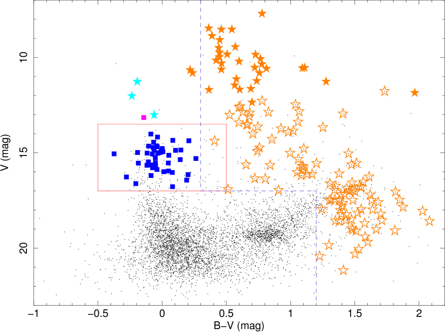
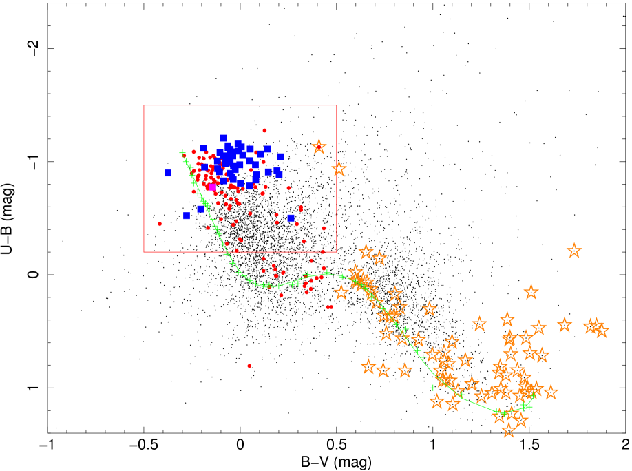
Figure 10: Colour-magnitude (left) and colour-colour (right) diagram. Black points show all possible optical counterparts of X-ray sources with measured $U$, $V$, and $B$ magnitudes in the MCPS found inside the $3\sigma$ positional uncertainty. Counterparts for Galactic foreground star candidates were selected redwards of the blue dashed line only. The red boxes mark the selection region of counterparts for BeXRBs in both plots. Identified foreground stars (filled orange stars), classified foreground stars (open orange stars), identified BeXRBs (blue squares) are marked. WR stars in the SMC and SMC X-1 are shown by cyan stars and the magenta square. Red dots in the right diagram mark all sources (black dots) within the red box of the left diagram. The green line gives the colours for the unreddened main sequence according to Fitzgerald (1970).

Figure 11: Distribution of spectral classes of X-ray emitting stars.

6.3.1 Identification of Be/X-ray binaries

We identified 49 HMXBs listed in literature (e.g. Haberl & Sasaki 2000; Galache et al. 2008). During our survey, two new X-ray pulsars were discovered (Coe et al. 2011; Sturm et al. 2011a), as well as two further bright BeXRB transients (sources № 2732 and 3115, Coe et al. 2012). Although detected with XMM-Newton, the catalogue does not contain the source SXP 11.5, since it was not observed in the nominal field of view and therefore was not accessible to our processing (Townsend et al. 2011). The same holds for SXP 1062, which was recently discovered in the outer wing of the SMC (Hénault-Brunet et al. 2012; Haberl et al. 2012b) after our data processing. All other pulsars with known position are within our main field. A detailed analysis of the observed BeXRB population will be discussed in a forthcoming study. Our catalogue contains 200 detections of 42 X-ray pulsars. X-ray pulsations confirm the neutron star nature of the accreting object. Hardness ratios for all X-ray pulsars are shown in Fig. 8b in black. All other 17 detections of 8 HMXBs with unknown pulse period are plotted in green.

6.3.2 Search for Be/X-ray binary candidates

Sources are classified as HMXB candidates ($<$HMXB$>$), if they fulfil the following criteria:

(i) Because of the power-law-like X-ray spectrum, with a typical photon index of $\Gamma\sim 1$ (Haberl & Pietsch 2004), HMXBs can easily be discriminated from soft X-ray sources, by using the same dividing line as in Fig. 8a. In general, HMXB show a harder X-ray spectrum than AGN ($\Gamma\sim 1.7$), thus providing a lower limit for $HR_{3}$ at $-0.3$ (see Fig. 8b). There is a notable exception, SXP 8.02, where all detections of this pulsar lie outside the selection region of Fig 8b. This can be explained on the basis of the anomalous X-ray pulsar (AXP) nature of this object (Tiengo et al. 2008). The colours of SXP 22.1 (№ 935) have large uncertainties. In total 1536 XMM-Newton sources that are not identified as HMXB or AGN (see Sec. 6.4) are hard (see Table 2) X-ray sources with $HR_{3}>-0.3$.

(ii) To avoid chance correlations with sources having a high positional uncertainty, we only used X-ray sources with a positional uncertainty $<$2.5″. This excludes 33 X-ray sources.

(iii) In addition to the selection of X-ray colours, we searched for an early-type star as counterpart. We used the loci of the confirmed BeXRBs (shown with blue squares) on the colour-magnitude and colour-colour diagram of Fig. 10, to define the selection area for candidate BeXRB systems. The loci are indicated with red boxes and correspond to 13.5 mag $<V<$17 mag and colours of $-0.5$ mag $<B-V<$0.5 mag and $-1.5$ mag$<U-B<$$-0.2$ mag. The MCPS catalogue comprises 16 605 entries, which fulfil these criteria and are in the XMM-Newton field.

(iv) To further improve the discrimination between AGN and HMXB, we use a third dividing line in the $HR_{3}$-$HR_{4}$-plane (Fig. 8f), where the difference in average power-law photon index has most effect. We note, that the separation between BeXRB and AGN population is not clear-cut. Highly obscured AGN are shifted towards larger $HR_{3}$, and there are also some detections of HMXB on the left side of the cut. We find 34 sources fulfilling the criteria i$-$iv above. By using subsamples of XMM-Newton and MCPS sources fulfilling the criteria i$-$iv and shifting the coordinates of one catalogue as described in Sec.5.2, we estimate $\sim$16.6$\pm$3.4 chance coincidences.

(v) Two weak candidates (№ 154 and 1408) correlate with emission-line objects, confirming the possible HMXB nature of these sources.

Five sources that fulfil the criteria i$-$iii, but violate criteria iv and v, are considered as weaker candidates, and are marked with “?”. In addition, we found one source, № 66, in the young star cluster NGC 330, but due to the high stellar density, no optical counterpart could be identified in the MCPS at this position. However, the source correlates with the Be star NGC 330:KWBBe 224 (Keller et al. 1999). The hardness ratios and short-term variability further support the HMXB nature of this source. Source № 1605 is in the star cluster NGC 376 and was rejected because of a $B-V$=0.71 in the MCPS. However, this colour might be influenced by confusion with other stars in the cluster. We find $B-V=-0.15$ in the OGLE catalogue (Udalski et al. 1998) and a classification of B2e by Martayan et al. (2010). Source № 823 was rejected because of a $B-V$ colour of 2.4 mag in the MCPS, although this source was classified as B1-5 III e by Evans et al. (2004) and has $B-V=-0.13$ in the OGLE catalogue. Source № 3003 is outside the MCPS field. Its X-ray properties and optical colours from Massey (2002) are also consistent with a HMXB (Sturm et al. 2013b). Evans et al. (2004) classified the optical counterpart as B1-3 III. Therefore, we also add these four sources to the catalogue of HMXB candidates.

All 45 candidate HMXBs ($<$HMXB$>$) are listed in Table 5. This list includes also the weak candidates as they are useful to set an upper limit to the BeXRB luminosity function.

Table 5: HMXB candidates in the SMC.

X-ray						MCPS				MA93		Comments
No	RA	Dec	ePos	$V$	$Cst$	$d$	$V$	$B-V$	$U-B$	$d$	No	and
	(J2000)	(J2000)	(″)		(%)	(″)	(mag)	(mag)	(mag)	(″)		references
12	01 19 38.94	-73 30 11.4	0.7	1.8	34.4	0.3	15.8	-0.1	-0.8	0.9	1867	H00, SG05
65	00 57 23.66	-72 23 55.8	0.8	6.4	13.0	1.7	14.7	-0.1	-1.0	–	–	?, SG05, A09
66	00 56 18.85	-72 28 02.7	0.7	1.3	0.2	–	–	–	–	–	–	in NGC 330, SG05
94	00 55 07.72	-72 22 40.3	0.9	1.9	20.7	0.8	14.4	-0.1	-1.0	–	–	L10
117	00 48 18.73	-73 20 59.9	0.6	2.3	4.4	0.2	16.2	0.3	-0.8	–	–	SG05, A09, K09
133	00 50 48.06	-73 18 17.6	0.9	3.4	8.3	0.3	15.1	0.1	-1.0	2.8	396	SG05, A09
137	00 52 15.06	-73 19 16.3	0.6	2.2	0.0	2.2	15.9	-0.1	-1.0	5.7	552	L10
154	01 00 30.26	-72 20 33.1	1.0	4.4	12.4	0.7	14.6	-0.1	-1.0	0.3	1208	SPH03, SG05
160	01 00 37.31	-72 13 17.4	0.9	2.7	73.5	2.4	16.7	-0.2	-0.9	–	–	N03,SG05
247	01 02 47.51	-72 04 50.9	0.8	5.1	14.5	0.5	16.0	-0.3	-1.1	–	–	SXP 523 (W12,S13a)
259	01 03 28.54	-72 06 51.4	0.7	6.3	4.4	1.9	16.5	-0.2	-0.9	–	–	SG05, eclipsing (W04)
287	01 01 55.89	-72 10 27.9	0.9	12.1	0.1	0.9	15.1	-0.2	-0.9	–	–
337	00 56 14.65	-72 37 55.8	0.8	1.8	3.9	0.7	14.6	0.1	-1.3	1.9	922	SG05
474	00 54 25.99	-71 58 24.1	0.8	–	53.3	2.4	16.6	-0.1	-0.8	–	–	?
562	01 03 31.73	-73 01 44.4	1.0	3.3	0.3	1.5	15.4	-0.2	-1.1	–	–
823	01 00 55.85	-72 23 20.3	1.0	6.6	71.9	1.1	15.6	2.4	–	–	–	B1-5 III e
1019	00 49 02.67	-73 27 07.4	1.6	3.3	41.9	3.5	15.8	-0.2	-0.9	–	–
1189	01 03 33.62	-72 04 17.5	1.7	–	–	4.9	16.1	-0.1	-1.0	–	–
1400	00 53 41.76	-72 53 10.1	0.8	12.4	2.8	2.2	14.7	0.1	-1.1	–	–
1408	00 54 09.28	-72 41 43.2	1.4	1.7	53.4	1.3	13.8	-0.0	-0.7	1.0	739
1481	00 42 07.77	-73 45 03.4	0.7	–	0.0	1.5	16.8	-0.1	-0.5	–	–	B1-5 III (E04)
1524	00 45 00.20	-73 42 46.7	1.7	–	10.4	1.5	15.6	0.0	-0.3	–	–
1605	01 03 55.08	-72 49 52.7	1.5	–	89.2	3.7	16.2	0.7	-0.6	–	–	B2e, in NGC 376
1762	01 03 38.00	-72 02 15.5	1.6	3.8	13.7	4.5	16.3	-0.2	-0.8	–	–
1817	00 54 08.68	-72 32 07.5	1.4	–	12.6	1.1	16.9	-0.1	-0.3	–	–
1820	00 53 18.52	-72 16 17.6	1.6	–	98.9	2.3	16.6	-0.2	-0.8	–	–
1823	00 53 14.81	-72 18 47.6	1.7	–	12.8	4.9	16.6	-0.0	-0.8	–	–	L10
1826	00 52 35.29	-72 25 20.8	1.6	–	32.0	5.7	14.9	-0.2	-0.9	–	–
1859	00 48 55.55	-73 49 46.4	0.6	–	8.8	1.3	14.9	-0.2	-0.7	–	–	SG05
1955	00 55 35.02	-71 33 40.9	1.3	–	17.8	4.7	16.1	-0.1	-0.8	–	–
2100	01 04 48.54	-71 45 41.5	1.6	–	84.0	4.3	16.9	0.4	-0.2	–	–
2208	00 56 05.48	-72 00 11.1	2.0	–	6.8	1.3	16.7	-0.1	-0.9	–	–	N11
2211	00 55 07.25	-72 08 25.7	1.7	–	18.8	3.9	16.9	-0.1	-0.7	–	–
2300	00 56 13.87	-72 29 59.7	1.0	3.9	2.0	0.7	14.5	0.0	-1.0	–	–	B0.5 V e (E06)
2318	00 56 19.02	-72 15 06.1	1.8	–	97.9	5.2	16.1	-0.1	-0.9	4.7	928
2497	00 43 15.87	-73 24 39.2	1.5	–	11.8	2.7	16.7	-0.1	-0.8	–	–
2569	00 51 46.12	-73 07 04.3	1.1	1.4	7.0	2.9	16.7	-0.0	-0.7	–	–	?
2587	00 52 59.47	-72 54 02.1	2.1	7.4	–	1.7	16.8	0.2	-0.5	–	–
2675	00 55 49.77	-72 51 27.1	1.5	1.4	–	1.0	16.5	-0.0	-0.6	–	–	eclipsing (W04)
2721	01 06 00.78	-72 33 03.7	1.9	4.5	11.8	2.0	16.3	-0.1	-0.9	–	–
2737	01 08 20.18	-72 13 47.1	0.7	–	72.0	2.2	14.7	-0.1	-0.7	–	–	?, B5 II (E04)
3003	01 23 27.46	-73 21 23.4	1.1	–	20.9	1.3	15.5	-0.1	-0.9	–	–	B1-5 III (E04), S13b
3052	01 11 08.59	-73 16 46.1	0.7	–	36.1	0.1	15.5	-0.1	-1.0	–	–	SXP 31.0 ?, B1-5 II e (E04)
3271	00 51 33.27	-73 30 12.2	1.5	–	16.4	4.4	16.6	0.1	-0.8	–	–
3285	01 04 29.42	-72 31 36.5	1.3	8.2	70.8	1.4	15.8	-0.2	-1.1	–	–

(H00) Haberl & Sasaki (2000); (SPH03) Sasaki et al. (2003); (E04) Evans et al. (2004); (E06) Evans et al. (2006); (W04) Wyrzykowski et al. (2004); (SG05) Shtykovskiy & Gilfanov (2005); (K09) Kozłowski & Kochanek (2009); (A09) Antoniou et al. (2009); (N03) Nazé et al. (2003); (L10) Laycock et al. (2010); (N11) Novara et al. (2011); (W12) Wada et al. (2012); (S13a) Sturm et al. (2013a); (S13b) Sturm et al. (2013b).

6.4 Active galactic nuclei

Galaxies with an AGN are bright X-ray sources at cosmological distances, and constitute the majority (71% classified) of point sources in our catalogue. X-rays are caused by accretion onto a super-massive black hole. In the XMM-Newton energy band, AGN show power-law-like spectra with a typical photon index of 1.7. Different spectral properties of AGN strongly depend on the inclination of the AGN (Urry & Padovani 1995). In addition to studying the AGN itself, identified AGN in the background of the SMC offer reference positions for proper motion studies, and might be used to probe the absorption by the interstellar medium of the SMC.

6.4.1 Identification of AGN

Forty seven spectroscopically confirmed quasars could be identified in our catalogue, mainly from Véron-Cetty & Véron (2006) and Kozłowski et al. (2011). All XMM-Newton detections of these sources are plotted in Fig. 8c in black. Point sources, emitting X-rays and radio, are also dominated by AGN. We identified 25 X-ray sources, which correlate with radio background sources of Payne et al. (2004). Also in this case the number of expected chance correlations is low. These sources are appended with an additional r to their classification. In Fig. 8c, detections of these sources are plotted in magenta.

6.4.2 Classification of AGN

AGN can be separated well from stars in the $HR_{2}$–$HR_{3}$-plane (Fig. 8c). We selected AGN candidates ($<$AGN$>$) among hard X-ray sources, where we use the same cut as for stars to discriminate between soft and hard X-ray sources (red line in Fig. 8c). We could classify 16 AGN, which have a SUMSS radio counterpart (noted with r), but no correlation with a radio source of the SMC or foreground in Payne et al. (2004). For 110 sources, we found a hard X-ray source correlating with an infra-red selected AGN candidate of Kozłowski & Kochanek (2009, noted with i), in addition to the already identified AGN. Using the Chandra Wing survey, the optical counterparts can be determined more precisely, and we found 126 hard X-ray sources, correlating with Chandra sources and classified as AGN by McGowan et al. (2008, noted with x).

In general, one expects for the optical and X-ray flux of an AGN a ratio of $-1<\log(f_{X}/f_{O})<1$ (Maccacaro et al. 1988). Another 1861 X-ray sources were classified with $<$AGN$>$, if the source has an optical counterpart candidate with $\log(f_{X}/f_{O})>-1$ in the MCPS (noted with o). We stress, that this last classification is very general, because of the high source density in the MCPS. Chance correlations with stars in the SMC can result in fulfiling the same $\log(f_{X}/f_{O})$ criterion. Also, for weak X-ray sources, the optical luminosity of the AGN can be below the completeness limit of the MCPS. Since the bulk of hard X-ray sources are expected to be of the AGN class, this classification will be correct in most cases (cf. Sec. 7.2), but some sources may be of a different nature. Therefore we mark AGN classifications, based only on the optical criterion with a “?”.

6.5 Galaxies

Galaxies behind the SMC can be seen in X-rays, comprising an unresolved combination of different X-ray sources, e.g. X-ray binaries, SNRs, diffuse emission, and a contribution of a central AGN. In the 6dFGS (Jones et al. 2009), we found 6 entries, correlating with X-ray sources (№ 365, 376, 645, 1726, 2905, and 3208). These sources were classified as galaxies, with the exception of № 365 (6dFGS gJ005356.2-703804), which was identified as AGN in the previous section. Source № 1711 was fitted as an extended source in X-rays and also has a counterpart in the 2MASS extended source catalogue (2MASX, Skrutskie et al. 2006), similar to the nearby source № 1726. There is an indication of diffuse emission in the mosaic image connecting both sources. Also sources № 708 and № 709 are inside a cluster of galaxies (ClG) and have 2MASX counterparts. Therefore, we also classified these sources as galaxies. Sources classified as galaxies are plotted in green in Fig. 8c. We did not find any redshift-confirmed galaxies in the SMC bar.

6.6 Clusters of galaxies

Clusters of Galaxies and galaxy groups contribute to the background sources. For a review see Rosati et al. (2002). The hot intra-cluster medium with temperatures of $kT\sim(2-10)$ keV causes thermal X-ray emission. Just like SNRs in the SMC, ClGs have an extent detectable with XMM-Newton. Since the temperature of SNRs is significantly lower, these two source classes can be separated by hardness ratios. The hardness ratios of all detections, which were flagged as significantly extended (QFLAG=E) in the X-ray images, are plotted in Fig. 8d. Only SNRs, super bubbles, and ClGs are expected as X-ray sources with such a large extent in the SMC field. Diffuse emission of the hot interstellar medium in the SMC is modelled by spline maps and treated as background. Identified SNRs and new candidates of Haberl et al. (2012a) are plotted in black. They have similar soft X-ray colours as stars. All other sources are plotted in green and show X-ray colours typical of ClGs in the mosaic image (cf. Haberl et al. 2012a). The red line marks our selection cut for the ClG classification. The only SNRs within this cut are IKT 2, IKT 4 and IKT 25. In addition to X-ray colours, we require a significant extent of the X-ray source of $Ext>\Delta Ext$ and a maximum likelihood for the extent of $ML_{\rm ext}>10$ for a CIG classification. Using these criteria, we classified 13 of 19 sources with significant extent as ClG candidates ($<$ClG$>$), in addition to the 11 ClGs not included in the point-source catalogue (because of their very large extent). All sources with significant extent are listed in Table 6.

6.7 Other source classes

The search for additional source classes is more extensive and will be discussed in other studies. This includes fainter low-mass X-ray binaries or cataclysmic variables in the SMC that are at the detection limit of the XMM-Newton survey. Extended sources, such as SNRs and ClGs, which are not included in our catalogue, are presented in Haberl et al. (2012a). A search for highly absorbed X-ray binaries in the survey data was presented by Novara et al. (2011). Candidates for highly absorbed white dwarf/Be systems are listed in Sturm et al. (2012). We assigned a specific source class to some individual sources: Source № 48 as an anomalous X-ray pulsar (AXP, Tiengo et al. 2008), source № 54 as a pulsar wind nebula or micro quasar (PWN?/MQ?, Owen et al. 2011), source № 324 as an isolated neutron star candidate (INS?, Kahabka & Haberl 2006), source № 551 as PWN candidate (PWN?, Filipović et al. 2008), and source № 535 as a star cluster (Cl*, Sec. 6.1.3).

7 General characteristics of the dataset

With the XMM-Newton catalogue of the SMC, the central field is covered completely down to a luminosity of 5$\times 10^{33}$ erg s^-1 in the (0.2$-$4.5) keV band, deeper than with previous imaging X-ray telescopes. The comparison with previous ROSAT and Chandra surveys, as well as with the XMM-Newton Serendipitous Source Catalogue, shows that $\sim$1200 sources have been detected for the first time during the large-programme SMC survey. Some basic properties of the dataset will be discussed in the following sections.

7.1 Spatial distribution

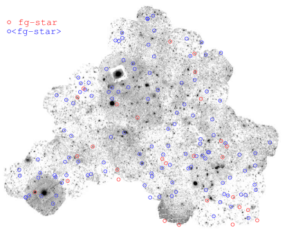
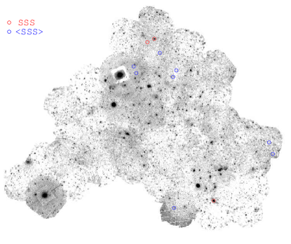
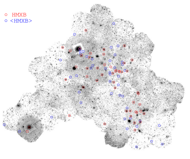
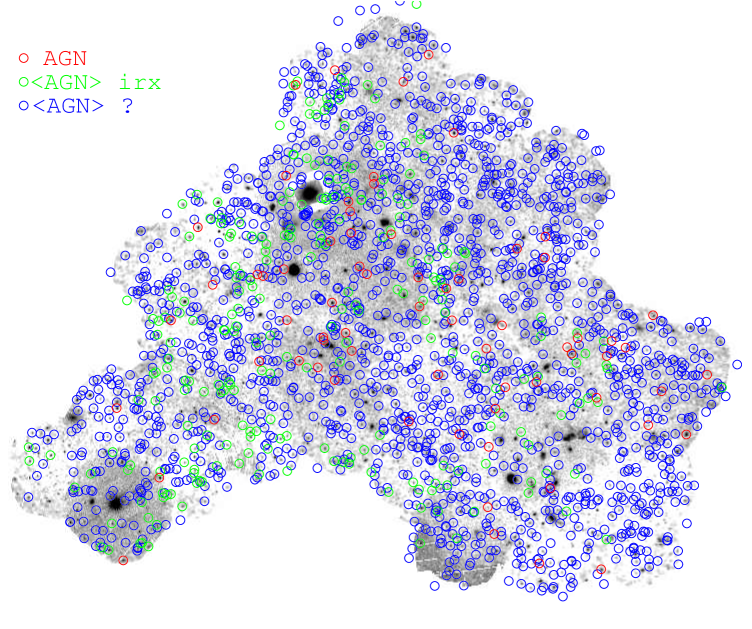
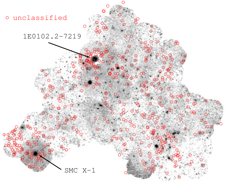
Figure 12: Spatial distribution of identified and classified X-ray sources in the SMC main field. The underlying mosaic image shows logarithmically scaled intensities in the (0.2–4.5) keV band. North is up, east is left.

The spatial distribution of individual source classes in the main field is shown in Fig. 12. In the upper left, sources identified as Galactic stars (red) or classified as candidates for Galactic stars (blue) are marked. The distribution is homogeneous over the entire field. SSSs as well as SSS candidates (upper right) are found in the outer regions of the bar, especially in the northern part. We did not find any in the SMC wing. As expected, HMXBs and their candidates follow the SMC bar (middle left). Since the bar harbours most of the blue main-sequence stars, we find here also most of the chance correlations with background AGN that contribute to the HMXB candidates. AGN show a homogeneous distribution over the observed field (middle right). Infrared selected AGN candidates are restricted to the smaller Spitzer S³MC field, AGN candidates from Chandra are only in the Chandra Wing fields. Clusters of galaxies that could be identified or classified, are shown in the lower left. Unclassified sources are marked in the lower right. Here we see some enhancement at the eastern rim, where the MCPS does not cover the field, and around SMC X-1, which may cause some spurious detections due to its brightness. Also around 1E0102.2-7219, an enhancement of unclassified sources is observed, as expected, due to the high number of observations, which lead to a higher number of spurious detections.

7.2 Luminosity functions

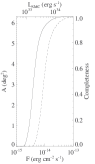
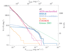
Figure 13: Left: Sky coverage as function of flux is shown for the (0.2–12.0) keV and (2.0–12.0) keV band by the solid and dashed line, respectively. Right: Cumulative luminosity function for sources and their classification in our catalogue (solid lines) and according models (dashed lines) as described in Sec. 7.2.

We constructed the luminosity function of the various classes of objects detected in the SMC fields. For sources with high long-term time variability, taking the average or maximal flux would not represent the source luminosity distribution of the galaxy at one time. For each source, we selected the flux from the observation with the highest sensitivity at this position, i.e. with minimal detection-limit flux. If the source was not detected in this observation, the source was not taken into account for the luminosity function. None of the selected detections is from an observation that was triggered by an outburst of the corresponding source. Therefore, this method selects one of several measured fluxes of transient sources in a quasi-random manner and thus represents the flux distribution as measured in one single observation of the whole galaxy. Also, this method minimises the effect of spurious detections at higher fluxes, since the source has to be detected in the most sensitive observation.

Depending on exposure time and observation background, the sensitivity varies between individual observations. Diffuse emission and vignetting also cause a spatial dependence of the sensitivity within each observation. The calculation of sensitivity maps is described in Sec. 3.3. To estimate the sky coverage, we merged all sensitivity maps, by selecting the observation with highest sensitivity at each position. The corresponding completeness function is presented in Fig. 13, left.

Especially for background sources, the completeness for the full energy band is clearly overestimated, since the ECFs adopted from the universal spectrum (Sec. 3.2) only account for galactic absorption, but not for absorption in the SMC, reaching line-of-sight column densities of up to $1.4\times 10^{22}$ cm^-2. To minimise this effect, we use the (2.0$-$12.0) keV band in the following. The flux reduction by Galactic absorption ($\sim$$6\times 10^{20}$ cm^-2) is 0.5% for the assumed universal spectrum, so we use the observed fluxes here. The completeness-corrected cumulative distribution of all sources is shown by the solid black line in Fig. 13, right. The correction mainly affects the number of sources with fluxes below $\sim 3\times 10^{-14}$ erg cm^-2 s^-1, as can be seen by the uncorrected distribution (dotted line).

For HMXBs, we see a break around $10^{-12}$ erg cm^-2 s^-1, similar to that inferred by Shtykovskiy & Gilfanov (2005). As suggested by these authors, this can be caused by the propeller effect, which can inhibit accretion at low accretion rates. Using C statistics, we parameterise the flux distribution of the total (i.e. not normalised by area) HMXB populations by fitting a broken power law to the unbinned source counts:

$$n(F)=\frac{dN}{dF}=\left\{\begin{array}[]{lll}N_{1}\,F^{-\alpha_{1}}&{\rm if}&F\leq F_{b}\\ N_{2}\,F^{-\alpha_{2}}&{\rm if}&F>F_{b}\\ \end{array}\right.$$

with the faint and bright end slopes $\alpha_{1}$ and $\alpha_{2}$, the normalisation $N_{2}=N_{1}F_{b}^{\alpha_{2}-\alpha_{1}}$, and the break flux $F_{b}$ and flux $F$ in 10^-12 erg cm^-2 s^-1. For HMXBs, we obtain $\alpha_{1}=0.64_{-0.17}^{+0.13}$, $\alpha_{2}=3.30_{-1.38}^{+2.17}$, $F_{b}=2.09_{-1.21}^{+0.74}\times 10^{-12}$ erg cm^-2 s^-1, and $N_{1}=11.9_{-3.5}^{+7.5}$. Including the HMXB candidates as well, we obtain $\alpha_{1}=0.87_{-0.10}^{+0.08}$, $\alpha_{2}=3.52_{-1.64}^{+1.91}$, $F_{b}=2.25_{-1.49}^{+0.62}\times 10^{-12}$ erg cm^-2 s^-1, and $N_{1}=13.9_{-3.4}^{+7.6}$.

Uncertainties are for 90% confidence. These models are shown by the blue dashed lines in Fig. 13 and give an upper and lower limit for the luminosity function. The bright-end slope is significantly steeper than found for HMXB populations of nearby galaxies above a luminosity of $10^{38}$ erg s^-1 ($\alpha=1.61\pm 0.12$, Grimm et al. 2003). The extrapolation of this model to lower luminosities is shown by a dashed green line in Fig. 13, where we used a star-formation rate of SFR${}_{\rm SMC}=0.15$ M_☉ yr^-1 (as in Grimm et al. 2003) and a correction factor of 1.24 (as expected for a photon index of $\Gamma=1$) to obtain fluxes in the (2.0–12.0) keV band. Mineo et al. (2012) suggest that this model is valid down to $L_{X}\sim 10^{35}$ erg s^-1. The deviation is probably caused by different source types. Our sample is dominated by BeXRBs, which show outbursts above luminosities of $10^{36}$ erg s^-1, whereas for more distant galaxies, due to higher flux limits only the brightest HMXBs can be detected. These contain a higher fraction of supergiant HMXBs which are, compared to BeXRBs, rather persistent and can contain a black hole instead of a neutron star.

Indeed, the presence of one supergiant system in the SMC, SMC X-1, is consistent with the Grimm model. In this context, the turn over might be interpreted as the transition from transient to persistent BeXRBs. We do not discuss the luminosity function below $\sim 2\times 10^{-14}$ erg cm^-2 s^-1, as we have only 3 sources here and run into incompleteness issues.

For background sources, we compare the SMC field with the XMM-Newton COSMOS field (Hasinger et al. 2007). The COSMOS-field source counts and broken power-law model of Cappelluti et al. (2009) is shown in red in Fig. 13. As these values are given in the (2.0–10.0) keV band, we applied a factor of 1.14 to estimate fluxes for the (2.0–12.0) keV band, as expected for a power law with photon index of $\Gamma=1.7$. For such a power law, we expect a flux decrease in the (2.0–12.0) keV band by 1.2% and 2.4% when crossing a column density of 5 and 10 $\times 10^{21}$ cm^-2 of ISM of the SMC, respectively. Analogously, we would expect a flux decrease by 35% and 51% (0.5–2.0) keV, for an AGN with negligible intrinsic absorption. We find a general agreement with the distribution of unidentified and AGN sources (magenta line in Fig. 13). Small deviations can be explained by the slightly different data processing. The contribution of Galactic stars (orange line in Fig. 13) is negligible above 2 keV.

7.3 Spectral properties

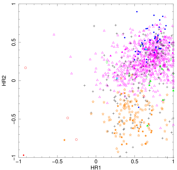
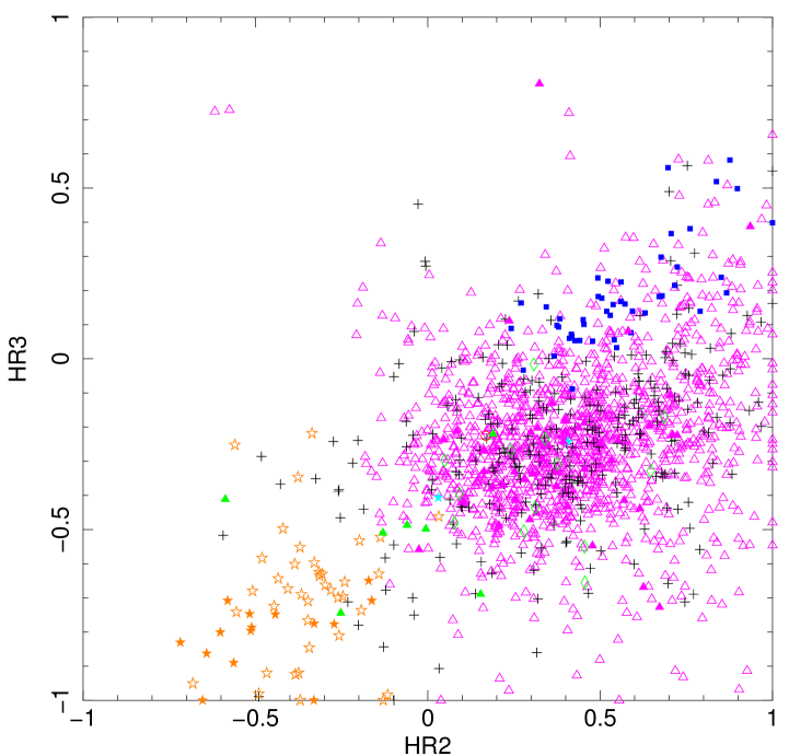
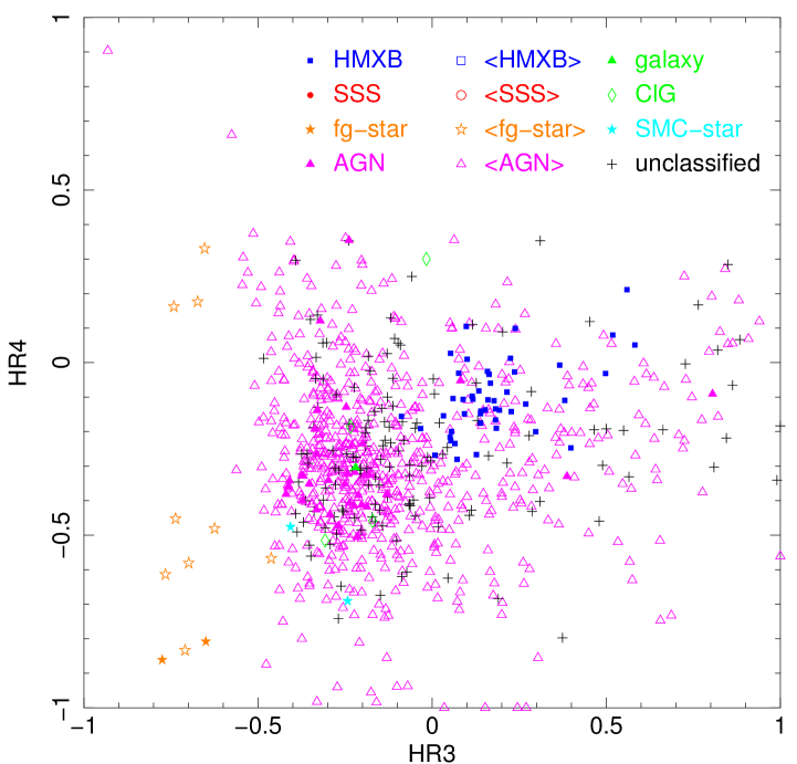
Figure 14: Hardness-ratio diagrams of all catalogue sources with respective uncertainties of $\Delta HR_{i}<0.25$, illustrating the spectral distribution of the catalogue sources.

To characterise the spectral properties of our source sample, we calculated hardness ratios as described in Sec. 3.2. Hardness-ratio diagrams of sources with well measured hardness ratios ($\Delta HR_{i}<0.25$) are presented in Fig. 14. Of course, the classified sources follow our selection criteria (cf. Fig. 8). In total we find 436 hard unclassified sources which are presumably mainly background AGN, where we expect a faint optical counterpart. If we assume a completeness of the MCPS catalogue of $V\approx 21$ mag, we can miss optical counterparts of AGN with $\log{(f_{x}/f_{o})}=1$ if they are fainter than $F_{x}=10^{-12.7}$ erg cm^-2 s^-1. Nearly all of the unclassified hard sources have such a low X-ray luminosity. A few hard sources might be caused by foreground flare stars, where the X-ray photon statistics is insufficient to detect variability. Also, the comparison with the COSMOS field (Fig. 12) seems to be consistent with most of these sources being background. Sources in the upper left of the $HR_{3}$-$HR_{4}$-plane are good candidates for highly absorbed AGN (Brightman & Nandra 2012), where the absorption can exceed N_H$>10^{24}$ cm^-2, which is significantly higher than expected from the interstellar medium of the SMC along the line of sight. From 130 unclassified soft sources, 67 have a detection likelihood of $ML_{\rm det}<10$. Here we expect most to be spurious detections. Other soft X-ray sources might originate from distant K or G stars that cannot be distinguished well from bright SMC stars and violate criterion iii of our foreground star selection.

7.4 Source extent

Table 6: Sources with significant extent.

SRC	RA	Dec	Ext (″)	$ML_{\rm ext}$	$HR_{2}$	$HR_{3}$	Class	Comment
1	01 17 05.2	-73 26 36	6.34 $\pm$ 0.02	69614.5	0.27 $\pm$ 0.00	0.16 $\pm$ 0.00	HMXB	pile-up
307	01 03 28.6	-71 45 48	8.74 $\pm$ 0.95	11.5507	0.34 $\pm$ 0.08	-0.23 $\pm$ 0.08	$<$ClG$>$
362	00 53 08.7	-72 34 45	10.90 $\pm$ 1.63	12.8268	-0.32 $\pm$ 0.12	-0.35 $\pm$ 0.20		in B0050-72.8
566	01 01 25.0	-72 46 34	14.20 $\pm$ 1.84	13.1577	0.31 $\pm$ 0.15	-0.02 $\pm$ 0.14	$<$ClG$>$
571	01 04 08.1	-72 43 54	20.24 $\pm$ 1.46	24.7586	0.65 $\pm$ 0.09	-0.33 $\pm$ 0.09	$<$ClG$>$
604	00 52 53.4	-73 00 09	3.74 $\pm$ 0.61	12.7043	-0.28 $\pm$ 0.06	-0.68 $\pm$ 0.09	$<$fg-star$>$	multiple stars?
638	01 09 53.3	-72 21 47	31.89 $\pm$ 2.87	20.3845	-0.26 $\pm$ 0.13	-0.38 $\pm$ 0.22		extent spurious?
799	00 59 04.1	-72 56 45	8.51 $\pm$ 1.05	29.0269	0.28 $\pm$ 0.07	-0.50 $\pm$ 0.08	$<$ClG$>$
916	01 16 15.3	-73 26 57	11.94 $\pm$ 1.11	45.9855	0.45 $\pm$ 0.08	-0.55 $\pm$ 0.09	$<$ClG$>$
937	01 13 53.2	-73 27 08	8.51 $\pm$ 1.00	11.7371	0.31 $\pm$ 0.09	-0.44 $\pm$ 0.10	$<$ClG$>$
1174	01 03 45.9	-71 54 36	14.79 $\pm$ 2.04	12.6019	0.69 $\pm$ 0.17	-0.17 $\pm$ 0.11	$<$ClG$>$
1305	01 01 26.3	-75 05 06	9.12 $\pm$ 1.40	18.3986	0.08 $\pm$ 0.12	-0.48 $\pm$ 0.15	$<$ClG$>$
1436	00 53 03.5	-70 47 34	12.48 $\pm$ 2.12	10.241	0.24 $\pm$ 0.17	-0.27 $\pm$ 0.17	$<$ClG$>$
1505	00 44 19.4	-73 36 24	13.15 $\pm$ 1.90	12.332	0.05 $\pm$ 0.14	-0.30 $\pm$ 0.17	$<$ClG$>$
1562	00 58 22.2	-72 17 59	19.94 $\pm$ 2.38	15.5316	0.08 $\pm$ 0.15	-0.50 $\pm$ 0.17	$<$AGN$>$ o?	in IKT 16
1711	01 09 00.6	-72 29 03	8.56 $\pm$ 1.03	23.5625	-0.25 $\pm$ 0.08	-0.74 $\pm$ 0.12	galaxy	in ClG?
2695	01 02 18.3	-72 37 03	12.57 $\pm$ 1.55	21.9732	0.38 $\pm$ 0.11	-0.31 $\pm$ 0.11	$<$ClG$>$
2889	01 13 26.3	-72 42 19	13.25 $\pm$ 1.64	26.7555	0.09 $\pm$ 0.13	-0.40 $\pm$ 0.17	$<$ClG$>$
3030	01 23 32.1	-73 17 10	8.35 $\pm$ 1.35	17.5979	0.46 $\pm$ 0.11	-0.65 $\pm$ 0.14	$<$ClG$>$

Table 6 lists all sources, fitted with a significant extent, where we demand $Ext>\Delta Ext$ and a likelihood for the extent of $ML_{\rm ext}>10$. Most of them are consistent with a ClG classification. Three other sources are inside or behind an extended X-ray source. In the case of SMC X-1 (№ 1), the source extent is caused by pile-up. For № 604, the hardness ratios point to a star. In the optical, several bright counterpart candidates are found. The extent might be due to a superposition of two or more stars. № 638 was detected as an extended source only in one of three detections. Therefore the extent might be spurious. We note that 13 additional sources were fitted with extent at lower likelihood or with high uncertainty.

7.5 Source variability

7.5.1 Intra-observational variability

To estimate the variability of sources during the individual observations, we used KS-tests as described in Sec. A.4. This allows us to estimate the source variability for sources with poor statistics. Some examples of cumulative count distributions, as used for the KS-test, are presented in Fig. 15. Here, we give the example of a bright star (№ 2041, upper left) showing a flare and a variable HMXB (№ 335 = RX J0054.9-7245, upper right). A foreground star candidate (№ 255, lower left), detected with only 29 counts, also exhibits a flare. As an example for a constant source, the SNR 1E0102.2-7219 is given in the lower right. In the case of high variability, the photon time distribution of the source (black line) shows a difference to the reference distribution for a constant source (red line), that is unlikely to be caused by statistical fluctuations.

The distribution of probabilities $Cst$ for constancy during individual observations is presented in Fig. 16 for various source classes. Here we see a uniform distribution, with the exception of stars and HMXBs. These are expected to show variability, whereas extended sources can be assumed to have a constant X-ray luminosity on short time scales. All 89 sources with $Cst<0.5\%$ are listed in Table 7. Assuming a uniform distribution we would expect $\sim$15 catalogue sources to be found with $Cst<0.5\%$ by chance. Whereas 15.4% of all HMXB detections and 9.3% of all foreground-star detections have $Cst<0.5\%$, this occurs only for 0.8% of the remaining detections.

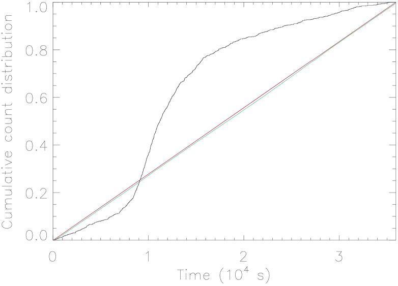
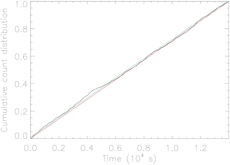
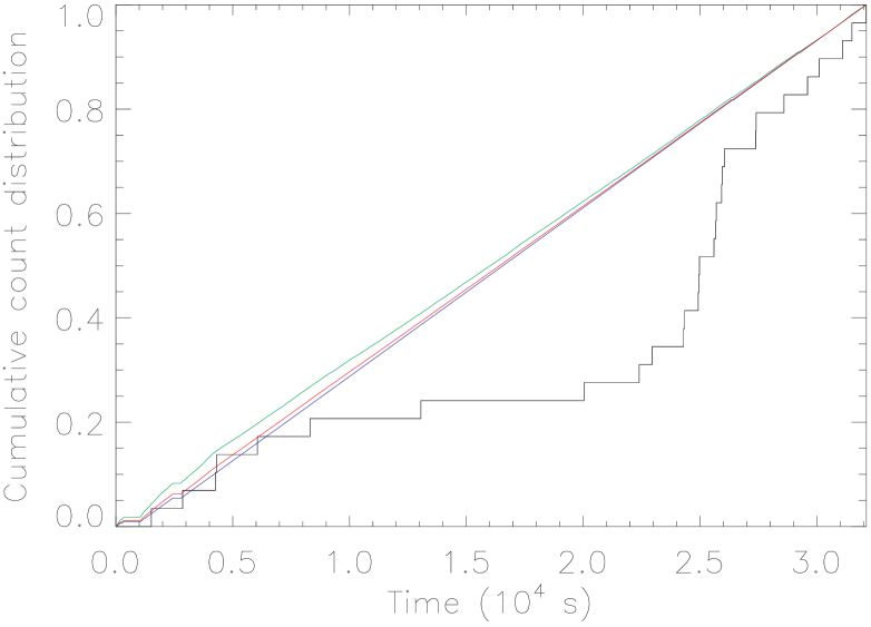
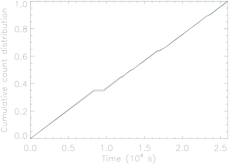
Figure 15: Cumulative photon arrival time distributions as used for the KS tests. Source counts are plotted in black, the background light curve is shown in green. The distribution, expected from a constant source is shown in blue and the reference distribution in red. In case of a constant source and background light curve, all lines are blended. The source-count distribution of variable sources is significantly different from the expected distribution. Upper left: The bright foreground star № 2041. Lower left: The foreground star candidate № 255. Upper right: The HMXB RX J0054.9-7245 (№ 335). Lower right: The SNR 1E0102.2-7219.

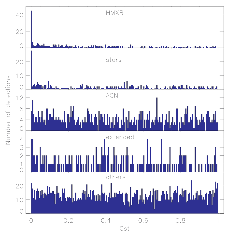
Figure 16: Histogram of probability that the source flux was constant within the observation. The bin size is 0.005. Note the number of stars and HMXB showing short-term variability with $Cst<0.5\%$ caused by the flaring behaviour of these source classes.

Table 7: X-ray sources in the SMC field with significant short-term variability.

SRC	RA	Dec	Class	$\log{(Cst)}$	$N$	SRC	RA	Dec	Class	$\log{(Cst)}$	$N$
1	01 17 05.2	-73 26 36	HMXB	$<$-40	316817	851	01 10 57.6	-73 05 14	$<$fg-star$>$	-13.06	290
2	01 18 38.0	-73 25 27	fg-star	-39.36	13873	852	01 16 33.5	-72 59 49	AGN	-5.51	1008
7	01 19 39.4	-73 27 33	$<$fg-star$>$	-3.63	171	884	01 00 13.9	-73 07 25	$<$fg-star$>$	-17.02	2022
9	01 16 27.9	-73 14 47	$<$AGN$>$ o?	-3.08	153	885	01 00 37.2	-73 00 36	$<$fg-star$>$	$<$-40	1067
37	01 14 55.6	-73 15 33	$<$fg-star$>$	-2.58	280	888	01 00 39.2	-73 16 55		-9.01	211
51	01 01 20.7	-72 11 19	HMXB	-3.73	1081	905	00 55 02.1	-73 21 15	$<$fg-star$>$	-15.30	290
61	00 55 35.4	-72 29 07	HMXB	-4.67	505	923	01 17 50.1	-73 30 09		-4.18	55
63	00 54 56.3	-72 26 47	HMXB	-3.37	463	934	01 16 35.0	-73 37 43	$<$AGN$>$ o?	-2.97	10
66	00 56 18.9	-72 28 03	$<$HMXB$>$	-2.70	214	937	01 13 53.2	-73 27 08	$<$ClG$>$	-2.38	119
92	00 54 46.3	-72 25 23	HMXB	-8.26	1160	948	01 16 21.7	-73 29 32		-13.49	33
112	00 47 23.3	-73 12 28	HMXB	-31.48	7094	1032	00 59 14.3	-72 20 12	$<$fg-star$>$	-4.87	21
113	00 51 52.2	-73 10 34	HMXB	-6.92	10189	1041	00 53 07.8	-74 39 06	fg-star	$<$-40	241087
137	00 52 15.1	-73 19 16	$<$HMXB$>$	-4.97	387	1194	01 05 46.8	-72 02 34	$<$AGN$>$ o?	-8.93	63
146	00 48 59.2	-72 58 17	$<$fg-star$>$	-13.08	214	1199	01 02 23.2	-72 11 35	$<$fg-star$>$	-2.59	11
149	00 57 49.4	-72 02 36	HMXB	$<$-40	6024	1399	00 55 18.3	-72 38 52	HMXB	-5.35	1551
165	00 59 40.8	-72 19 05		-2.47	22	1462	00 52 03.0	-72 05 05	$<$AGN$>$ o?	-2.40	219
183	00 58 58.7	-72 01 12	$<$fg-star$>$	-3.36	20	1481	00 42 07.8	-73 45 03	$<$HMXB$>$	-6.64	315
184	01 01 52.3	-72 23 33	HMXB	-6.16	999	1483	00 41 55.3	-73 34 16	$<$AGN$>$ o?	-2.35	131
187	01 03 14.0	-72 09 14	HMXB	-2.63	1322	1500	00 42 21.2	-73 27 58	$<$fg-star$>$	-8.80	29
197	01 05 09.9	-72 11 47	$<$AGN$>$ ox	-3.20	189	1525	00 44 18.5	-73 37 00	$<$AGN$>$ o?	-2.50	28
216	01 02 06.7	-71 41 16	HMXB	-7.85	1948	1560	00 43 02.2	-72 52 34	$<$AGN$>$ o?	-4.48	428
227	01 03 37.6	-72 01 33	HMXB	-9.15	7426	1617	01 02 08.0	-72 47 32	$<$AGN$>$ o?	-2.51	19
228	01 05 55.4	-72 03 49	HMXB	-3.57	235	1700	00 50 05.6	-73 32 01	$<$AGN$>$ o?	-2.31	30
231	01 01 37.7	-71 54 15	$<$fg-star$>$	-8.88	199	1702	00 49 13.5	-73 25 60	$<$fg-star$>$	-2.51	21
239	01 05 50.3	-71 57 60	$<$fg-star$>$	-2.74	65	1755	01 03 42.6	-71 57 58		-17.86	36
255	01 05 00.3	-72 11 48	$<$fg-star$>$	-4.26	29	1802	00 52 05.7	-72 26 05	HMXB	-2.32	2592
256	01 05 37.5	-71 57 19		-2.34	22	1998	00 50 12.1	-71 46 54	$<$fg-star$>$	-4.35	28
287	01 01 55.9	-72 10 28	$<$HMXB$>$	-2.95	28	2002	00 47 17.6	-71 55 20	$<$AGN$>$ o?	-2.54	42
335	00 54 55.9	-72 45 11	HMXB	-3.58	3038	2041	01 03 16.5	-71 31 42	$<$fg-star$>$	$<$-40	1014
352	00 53 24.2	-72 39 41	$<$AGN$>$ o?	-2.32	10	2381	00 42 38.8	-72 33 27	AGN r	-17.31	606
392	00 52 58.5	-70 50 22	$<$AGN$>$ o?	-2.55	19	2454	00 43 47.7	-73 02 08	$<$AGN$>$ o?	-2.42	27
402	01 09 30.0	-72 52 49	$<$AGN$>$ o?	-2.94	580	2601	00 56 45.4	-72 59 32		-5.50	154
407	01 08 25.9	-72 54 31	fg-star	-2.44	352	2651	00 54 50.8	-72 51 26	$<$AGN$>$ o?	-4.05	14
487	00 45 24.1	-73 29 07	$<$fg-star$>$	-4.39	451	2735	01 09 35.2	-72 11 45	fg-star	$<$-40	708
542	00 59 29.5	-71 58 09	$<$AGN$>$ oi	-2.66	31	2738	01 10 50.8	-72 10 25	AGN r	-2.66	332
556	01 02 14.7	-72 49 17	$<$AGN$>$ oi	-2.90	23	2740	01 09 18.6	-72 12 38	$<$fg-star$>$	-3.49	204
562	01 03 31.7	-73 01 44	$<$HMXB$>$	-2.49	19	2845	01 13 02.3	-72 41 42	$<$fg-star$>$	-9.22	524
615	00 49 30.6	-73 31 09	HMXB	-2.83	223	2846	01 11 54.6	-72 45 57	$<$fg-star$>$	-11.28	304
636	00 48 46.6	-73 30 00	$<$AGN$>$ o?	-2.62	16	3059	01 13 04.2	-73 14 35	$<$fg-star$>$	-9.03	103
654	00 53 23.9	-72 27 15	HMXB	-3.16	2149	3115	01 06 33.0	-73 15 43	HMXB	-11.24	811
668	00 54 38.5	-72 22 09	$<$AGN$>$ o?	-2.52	51	3167	01 02 28.0	-73 16 57	$<$AGN$>$ o?	-3.35	27
674	00 59 28.9	-72 37 04	HMXB	-14.16	6464	3186	00 59 37.0	-73 25 41	$<$AGN$>$ o?	-2.31	127
730	00 49 22.8	-72 10 55		-2.64	81	3190	00 58 35.7	-73 14 48	$<$fg-star$>$	-2.64	79
760	00 42 45.8	-73 10 14	$<$fg-star$>$	-2.79	173	3267	00 50 34.6	-73 30 30	$<$AGN$>$ o?	-6.26	214
812	01 00 09.6	-72 57 49	$<$AGN$>$ o?	-15.07	1087

7.5.2 Inter-observational variability

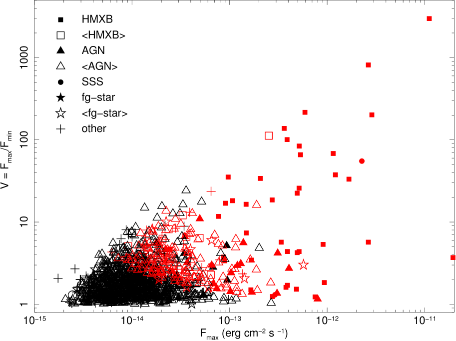
Figure 17: Variability of SMC sources as observed with XMM-Newton in the (0.2–4.5) keV band. Sources with a significance of variability greater (less) than 3 are plotted in red (black).

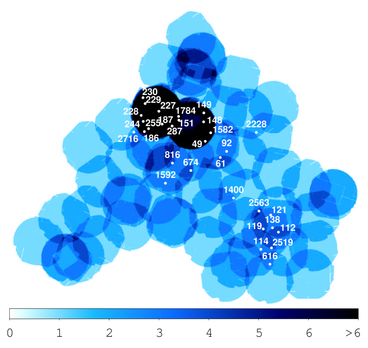
Figure 18: The number of observations per field is compared with the distribution of significant long-term variable sources ($V\geq 10$ and $S\geq 3$), shown by white dots. Labels give the source numbers. Variable sources are only found in the SMC bar in regions that have been observed several times.

For sources which were observed several times, the long-term variability was calculated as described in Sec. 3.2. The dependence of variability on the maximal detected flux is plotted in Fig. 17. For sources with $F_{\rm max}<10^{-14}$ erg cm^-2 s^-1, the variability is uncertain. The calculation results in a significant ($S\geq 3$) variability measurement for most sources with $F_{\rm max}$ above $10^{-13}$ erg cm^-2 s^-1.

Sources with high variability of $V\geq 10$ are listed in Table 8. As expected, most of these sources are HMXBs. For two HMXB candidates, the high variability supports their classification. In addition, we find the symbiotic nova SMC3, which has a known 1600 day variability, one Galactic star, possibly observed during a flare in one observation, and seven more sources, unclassified or with AGN classification. These sources show clear variability, which is rather high, but possible, for AGN (e.g. № 229 is identified as AGN). Another explanation of such high variabilities might be given by an X-ray binary nature, although we note that these sources do not have bright optical counterparts, needed for a HMXB classification. In the case of low-mass X-ray binaries (LMXBs), we would not expect to find an optical counterpart. Only very few LMXBs are expected in the SMC, as this population scales with the mass of the galaxy, and so far none are known, although the X-ray variable sources might be considered as candidates.

The spatial distribution of the highly variable sources is presented in Fig. 18. Obviously it is more likely to find variable sources in fields which were observed more frequently. Specifically, long-term variability cannot be measured in fields observed only once. Since most variable sources are HMXBs, the distribution follows the bar of the SMC.

Table 8: X-ray sources in the SMC field with high variability between individual observations.

SRC	Name	Class	$V$	$S$	$F_{\rm max}$
					($10^{-14}\times$ erg cm-2 s-1)
49	SXP 565	HMXB	216.4	6.5	59.22 $\pm$ 9.06
61	XMMU J005535.2-722906	HMXB	18.6	25.0	27.33 $\pm$ 0.91
92	CXOU J005446.2-722523	HMXB	33.9	27.8	20.65 $\pm$ 0.70
112	SXP 264	HMXB	37.6	66.7	121.59 $\pm$ 1.74
114	SXP 756	HMXB	22.4	38.5	49.25 $\pm$ 1.09
119	SXP 892	HMXB	16.4	10.8	14.76 $\pm$ 1.25
121	RX J0048.5-7302	HMXB	16.9	12.0	9.08 $\pm$ 0.69
138	SXP 25.5	HMXB	18.2	14.3	10.70 $\pm$ 0.69
148	SXP 152	HMXB	65.9	37.9	53.32 $\pm$ 1.38
149	SXP 280	HMXB	33.3	51.4	167.22 $\pm$ 2.68
151	SXP 304	HMXB	25.9	20.2	51.52 $\pm$ 2.25
186		$<$AGN$>$ oxr	16.1	14.6	18.90 $\pm$ 1.16
187	SXP 348	HMXB	100.8	31.2	38.84 $\pm$ 1.22
227	SXP 1323	HMXB	68.2	63.1	115.24 $\pm$ 1.79
228	RX J0105.9-7203	HMXB	35.3	13.7	9.67 $\pm$ 0.68
229	[VV2006] J010522.5-715650	AGN	11.0	9.7	4.95 $\pm$ 0.42
230			23.7	9.3	6.46 $\pm$ 0.66
244		$<$AGN$>$ o?	12.8	7.5	4.15 $\pm$ 0.50
255		$<$fg-star$>$	10.0	6.7	2.23 $\pm$ 0.29
287		$<$HMXB$>$	12.1	6.6	3.30 $\pm$ 0.45
616	SMC3	SSS	55.1	198.9	226.43 $\pm$ 1.08
674	XMMU J005929.0-723703	HMXB	201.5	67.0	286.67 $\pm$ 4.23
816	SXP 7.92	HMXB	11.7	6.9	7.71 $\pm$ 1.01
1400		$<$HMXB$>$	112.4	10.3	25.21 $\pm$ 2.43
1582		$<$AGN$>$ o?	10.9	3.8	2.79 $\pm$ 0.66
1592	SXP 6.85	HMXB	2990.9	167.0	1111.89 $\pm$ 6.65
1784			13.2	4.6	3.91 $\pm$ 0.78
2228	SXP 91.1	HMXB	84.1	51.0	51.72 $\pm$ 0.98
2519	SXP 11.87	HMXB	815.5	99.5	263.96 $\pm$ 2.65
2563	SXP 214	HMXB	137.9	32.9	36.31 $\pm$ 1.09
2716		$<$AGN$>$ o?	13.7	3.6	2.23 $\pm$ 0.57

8 Summary

For the first time, the central field of the SMC is fully covered to a limiting flux of $\sim$$2\times 10^{-14}$ erg cm^-2 s^-1 in the (0.2–12.0) keV band with an imaging X-ray telescope. 91 XMM-Newton pointings between April 2000 and April 2010 cover the bar and eastern wing of the SMC with an area of 5.6 deg² and a total net exposure of $\sim$2 Ms. We created a catalogue of 3053 unique X-ray point sources based on 5236 detections in the SMC field, including archival observations, providing spectral and temporal characteristics for all sources. The typical positional uncertainty of the sources in the catalogue is 1.3″. Cross correlations with other catalogues give distinct counterparts in X-ray and radio bands. In the optical, the selection of counterparts is challenging, due to the high stellar density in the SMC field. Most X-ray sources are background sources behind the SMC, namely AGN. We were able to positively identify 49 HMXB and 4 SSSs in the SMC together with 34 foreground stars and 72 background AGN. In addition we propose classifications for other sources based on their X-ray hardness ratios and positional cross-correlations with other catalogues, which often provided additional optical, infrared or radio characteristics. This resulted in likely identifications with foreground stars (128), HMXBs (45), faint SSSs (8) as well as AGN (2105) and galaxy clusters (13). This has allowed us to further investigate the X-ray source population of the SMC, in particular to derive the luminosity function of Be/X-ray binaries. This shows a significantly different bright end slope than expected from the universal HMXB X-ray luminosity function.

Appendix A Details of the catalogue creation

A.1 Catalogue screening

Each observation was screened individually and a quality flag QFLAG was set manually to indicate if the detection was most likely not caused by a point source. Spurious detections can be caused by single reflections of SMC X-1 (QFLAG=S), or by out-of-time events of bright sources (QFLAG=O). The substructure of extended sources, or residuals of the PSF of the brightest sources, can lead to multiple detections (QFLAG=M). Also, sources with significant extent, like SNRs and the largest clusters of galaxies, were marked (QFLAG=E) and not used for the catalogue.

Using a mosaic colour image of the SMC (Haberl et al. 2012a), we looked, in a second screening-step, for wrongly correlated detections and uncorrelated detections obviously originating from the same source. This occurred, for example, in the case of bright sources with low statistical uncertainty, if the astrometric solution was not yet sufficiently accurate. The EPIC-MOS CCDs show a significantly increased low-energy noise in some observations, if they are in an anomalous state (Kuntz & Snowden 2008). Affected CCDs were identified with emtaglenoise and the data were used for source detection, but not for the mosaic image. To ensure that the detections in these noisy CCDs are real, we required that the detection likelihood for the noisy CCD in the (1.0–12.0) keV band is sufficient for an independent detection, or that the source is found by an instrument not in anomalous state within the same, or another, observation. If, in addition, no source is visible in the mosaic image, the detection was flagged with QFLAG=N. Detections found in regions with enhanced diffuse emission, where the reliability is doubtful, were flagged (QFLAG=D) if no clear point source was visible in the deep mosaic image. The task epreject abolishes EPIC-pn offset map corrections for optical loading caused by bright optical sources with $V<12$ mag or $V<6$ mag for observations with thin or medium filter, respectively. We find 57 detections of 36 sources, which fulfil this criterion. If the source was not detected with a high level of significance by another instrument, in another observation, or in the EPIC-pn energy bands 2$-$5, we rejected this source (QFLAG=L). This caused a rejection of only 4 sources. All other 32 potentially affected sources show evidence for real X-ray emission. Sources, detected only in one observation and by only one instrument with detection likelihood $ML_{\rm det}>10$ in energy band 1, but not detected above 1 keV, were checked for hot pixels, which might have been missed by badpixfind and flagged (QFLAG=P) if a bright pixel was found in the detector image or if the detection was close to a hot pixel or column and had a peculiar, non-PSF-like, shape. All other detections have QFLAG=G, by default. Only the G-flagged sources were used for the creation of the point-source catalogue. The flags and the number of occurrences are listed in Table 9.

Table 9: Screening of detections.

QFLAG	Description	Number
G	good (default)	5236
M	multiple detection	503
S	single reflection	232
E	extended source	207
P	hot pixel	129
N	MOS CCD in anomalous state	110
O	out-of-time events	22
D	diffuse emission	20
L	optical loading	4

A.2 Astrometric corrections

The accuracy of the astrometric frame of XMM-Newton can be improved since the positions of bright sources have a higher statistical precision than the initial XMM-Newton attitude solution. However, the standard boresight correction, using a simple comparison with a complete optical reference catalogue, cannot be applied, because the number of chance correlations overwhelms the number of real counterparts in the SMC field. A first correction was applied to the event files, before the image creation (Haberl et al. 2012a). Using the autocorrelated detection list, we further improved the positions. We selected optical counterparts, mainly from Zaritsky et al. (2002), of identified HMXB and spectroscopically confirmed AGN, as well as identified foreground stars from the Tycho-2 catalogue (Høg et al. 2000), as described in Sec. 6. In the latter case, the proper motion was taken into account. We used this information to correct the spacecraft attitude for a linear boresight shift in right ascension and declination. The overall applied boresight corrections for all observations are listed in Table LABEL:tab:observations. As we only used identified sources instead of a general correlation with a reference catalogue, we also accepted coordinate corrections if only one identified source was available. This allowed a coordinate improvement for all observations.

A.3 Calculation of energy conversion factors

For the calculation of energy conversion factors (ECFs) $f_{i}=R_{i}/F_{i}$, we assumed a universal spectrum for all sources, described by a power-law model with a photon index of $\Gamma=1.7$ and a photo-electric foreground absorption by the Galaxy of $N_{\rm H,Gal}=6\times 10^{20}$ cm^-2 (average for SMC main field in H i map of Dickey & Lockman 1990). This spectrum was simulated with standard EPIC response matrix files (RMFs). We note that this universal spectral shape is only a rough assumption. Since the correction is from counts to detected flux, i.e. we do not report unabsorbed fluxes, and since the fluxes are calculated independently for each of the relatively narrow energy bands, deviations from the source spectrum over the total energy band are reduced. Therefore the calculated fluxes give a good approximation of the true detected flux in most cases (see also Pietsch et al. 2004).

For EPIC-MOS, an increased redistribution of measured photon energies is known to occur around the EPIC-pn and RGS prime pointing position, where most targets are placed (Read et al. 2006). This has some effect on the ECFs for the energy bands 1 and 2. We decided to use the off-patch single to quadruple event RMF, since in the case of the SMC survey, the majority of detections lies outside this patch area. The differences between on- and off-patch ECFs is $<$10% for energy band 1 and lower for the other bands. For EPIC-pn, the dependence of the spectral resolution on the detector position has an even smaller influence on the ECFs ($<$2%) and we used the RMF for CCD rows 81-100 as average. The dependence of the ECFs on data mode is $<$2% (Watson et al. 2009) and we used the full-frame RMFs for all instruments. The ancillary response files (ARFs) were calculated with arfgen for each filter and instrument and do not contain corrections, which have already been applied by emldetect. For EPIC-pn, $f_{5}$ is corrected for the screened (7.2–9.2) keV sub-band, thus translating to (4.5–12.0) keV fluxes. The derived ECFs are listed in Table 11. Since energy band 5 does not contribute substantially to the total flux, but rather increases its uncertainty in most cases, it is not used for the so-called XID flux (sum from band 1 to 4).

Table 10: Energy conversion factors.

Detector	Filter	$f_{1}$	$f_{2}$	$f_{3}$	$f_{4}$	$f_{5}$
pn	thin	11.150	8.132	5.839	1.943	0.463
	medium	9.976	7.897	5.758	1.926	0.465
	thick	6.329	6.071	4.964	1.824	0.459
MOS1	thin	2.118	1.937	2.064	0.744	0.144
	medium	1.891	1.883	2.029	0.735	0.144
	thick	1.273	1.530	1.807	0.705	0.142
MOS2	thin	2.117	1.938	2.070	0.748	0.152
	medium	1.886	1.884	2.034	0.740	0.152
	thick	1.264	1.530	1.812	0.710	0.150

A.4 Short-term time variability

To investigate the short-term time variability of all sources with KS-tests, we extracted time series of events of the EPIC-pn and both EPIC-MOS in the (0.2–4.5) keV band. Source counts were selected within an ellipse that approximates the PSF of the source at a surface brightness (in cts pix^-1) equal to the background surface brightness, as defined by the SAS task region. We merged the event lists in common GTIs of the individual EPIC instruments to obtain higher statistics. To estimate the background variability caused, for example, by residual soft-proton flares, we assumed a spatial independence of the background time variability. Background time series were extracted in a similar manner, but excluding regions around each point source where the PSF brightness is larger than 10% of the background value.

In most cases, the KS-test works well by using a linear increasing function during GTIs and a constant otherwise. In some cases, the background time series exhibits significant variability. To ensure that this has no influence on the variability estimation of faint sources, we created a reference function, combining the background and constant source distribution. The expected relative background contribution was estimated from the background maps (Sec. 3.1). Since the statistics of the background time series is high compared to that of faint sources, it can be used as a quasi-continuous function. We added this cumulative light curve to the constant-source function and performed a one-sample KS-test. The resulting probability, $Cst$, that the temporal photon distribution can be explained by a constant source was calculated for each detection. For sources with several detections, we give the minimum of $Cst$ over all detections. Sources that can be considered variable show values of $Cst<0.5\%$ (see Sec.7.5.1).

Appendix B List of used observations

1

Table 11: XMM-Newton observations of the SMC.

ID	ObsID	Target	Date			RA			Dec			$\Delta$RA	$\Delta$Dec	ExpID	Time			Filter	Mode	Exp	Net Exp
						(J2000)			(J2000)			(″)	(″)		(UT)					(s)	(s)
S1	0601210101	SMC survey 1	2009	May	14	00h	58m	16$\aas@@fstack{s}$4	-71°	28′	45″	1.42	0.85	M1S001	09:	14:	24	medium	ff	29419	4280
														M2S002	09:	14:	26	medium	ff	29425	4284
														PNS003	09:	36:	46	thin	ff	27512	3551
S2	0601210201	SMC survey 2	2009	Sep.	25	00h	53m	58$\aas@@fstack{s}$9	-71°	43′	48″	-0.91	0.1	M1S001	00:	15:	42	medium	ff	37420	37362
														M2S002	00:	15:	42	medium	ff	37425	37368
														PNS003	00:	38:	05	thin	ff	35834	35782
S3	0601210301	SMC survey 3	2009	May	18	00h	49m	01$\aas@@fstack{s}$8	-71°	56′	42″	0.53	-0.25	M1U002	10:	29:	15	medium	ff	31614	27589
														M2U002	10:	29:	34	medium	ff	31603	27580
														PNU002	10:	47:	01	thin	ff	30304	26332
S4	0601210401	SMC survey 4	2009	Sep.	25	01h	02m	59$\aas@@fstack{s}$3	-71°	36′	41″	-1.27	1.63	M1S001	11:	22:	24	medium	ff	37521	37464
														M2S002	11:	22:	23	medium	ff	37526	37469
														PNS003	11:	44:	46	thin	ff	35934	35882
S5	0601210501	SMC survey 5	2009	Sep.	25	00h	58m	54$\aas@@fstack{s}$9	-71°	49′	48″	0.47	-0.37	M1S001	22:	30:	43	medium	ff	50321	41464
														M2S002	22:	30:	43	medium	ff	50326	41469
														PNS003	22:	53:	05	thin	ff	48734	39923
S6	0601210601	SMC survey 6	2009	Sep.	27	00h	55m	20$\aas@@fstack{s}$2	-72°	01′	42″	-0.0	0.92	M1S001	00:	10:	53	medium	ff	38520	34617
														M2S002	00:	10:	53	medium	ff	38525	34622
														PNS003	00:	33:	16	thin	ff	36933	34278
S7	0601210701	SMC survey 7	2009	Sep.	27	00h	49m	28$\aas@@fstack{s}$7	-72°	17′	14″	0.78	0.82	M1S001	11:	35:	54	medium	ff	38621	38616
														M2S002	11:	35:	53	medium	ff	38626	38621
														PNS003	11:	58:	16	thin	ff	37034	37034
S8	0601210801	SMC survey 8	2009	Oct.	9	00h	56m	15$\aas@@fstack{s}$5	-72°	21′	55″	1.16	-0.34	M1S001	18:	33:	30	medium	ff	24620	24615
														M2S002	18:	33:	31	medium	ff	24625	24620
														PNS003	18:	55:	52	thin	ff	23034	23034
S9	0601210901	SMC survey 9	2009	Sep.	27	00h	48m	08$\aas@@fstack{s}$9	-72°	37′	39″	1.12	1.0	M1S001	23:	02:	34	medium	ff	41138	34083
														M2S002	23:	02:	33	medium	ff	41148	34091
														PNS003	23:	24:	56	thin	ff	39685	32742
S10	0601211001	SMC survey 10	2009	Nov.	9	00h	43m	56$\aas@@fstack{s}$7	-72°	44′	38″	-1.2	-2.56	M1S001	21:	16:	08	medium	ff	36520	26268
														M2S002	21:	16:	06	medium	ff	36525	26289
														PNS003	21:	38:	29	thin	ff	34934	24688
S11	0601211101	SMC survey 11	2009	Oct.	18	00h	42m	29$\aas@@fstack{s}$5	-73°	02′	27″	-0.1	-2.35	M1S001	22:	47:	09	medium	ff	31619	27114
														M2S002	22:	47:	09	medium	ff	31624	27119
														PNS003	23:	09:	31	thin	ff	30034	25534
S12	0601211201	SMC survey 12	2009	Oct.	20	00h	42m	25$\aas@@fstack{s}$2	-73°	20′	11″	1.82	0.06	M1S001	22:	51:	09	medium	ff	33119	29514
														M2S002	22:	51:	08	medium	ff	33124	29519
														PNS003	23:	13:	31	thin	ff	31534	27931
S13	0601211301	SMC survey 13	2009	Oct.	3	00h	46m	28$\aas@@fstack{s}$7	-73°	24′	25″	-0.36	-0.72	M1S001	05:	08:	47	medium	ff	32420	32363
														M2S002	05:	08:	46	medium	ff	32425	32368
														PNS003	05:	31:	10	thin	ff	30833	30779
S14	0601211401	SMC survey 14	2009	Nov.	4	00h	52m	19$\aas@@fstack{s}$2	-73°	09′	03″	0.89	0.67	M1S001	21:	38:	31	medium	ff	46520	32718
														M2S002	21:	38:	30	medium	ff	46525	32717
														PNS003	22:	00:	51	thin	ff	44290	31370
S15	0601211501	SMC survey 15	2009	Oct.	13	00h	56m	25$\aas@@fstack{s}$5	-73°	02′	58″	2.43	0.63	M1S001	00:	02:	01	medium	ff	37620	36863
														M2S002	00:	02:	00	medium	ff	37625	36868
														PNS003	00:	24:	22	thin	ff	36034	35280
S16	0601211601	SMC survey 16	2009	Oct.	11	00h	58m	21$\aas@@fstack{s}$5	-72°	48′	27″	0.71	-2.54	M1S001	22:	43:	47	medium	ff	43350	30443
														M2S002	22:	43:	46	medium	ff	43358	30443
														PNS003	23:	06:	08	thin	ff	41769	29100
S17	0601211701	SMC survey 17	2009	Oct.	16	01h	02m	23$\aas@@fstack{s}$1	-72°	35′	23″	1.37	1.36	M1S001	01:	05:	21	medium	ff	36738	20744
														M2S002	01:	05:	17	medium	ff	36785	20744
														PNS003	01:	57:	40	thin	ff	33664	17626
S18	0601211801	SMC survey 18	2009	Nov.	13	01h	04m	04$\aas@@fstack{s}$7	-72°	22′	52″	1.82	1.89	M1S001	20:	59:	56	medium	ff	2535	0
														M1U002	22:	23:	04	medium	ff	31531	22358
														M2S002	20:	59:	56	medium	ff	2540	0
														M2U002	22:	23:	11	medium	ff	31531	22377
														PNS003	21:	22:	19	thin	ff	34934	21659
S19	0601211901	SMC survey 19	2009	Nov.	30	01h	08m	33$\aas@@fstack{s}$2	-72°	09′	54″	0.19	0.86	M1S001	14:	46:	19	medium	ff	31619	31585
														M2S002	14:	46:	19	medium	ff	31624	31598
														PNS003	15:	08:	40	thin	ff	30034	30001
S20	0601212001	SMC survey 20	2009	Nov.	27	01h	12m	56$\aas@@fstack{s}$4	-72°	22′	38″	3.56	3.12	M1U002	22:	39:	06	medium	ff	28231	28126
														M2U002	22:	39:	09	medium	ff	28234	28113
														PNU002	23:	04:	04	thin	ff	26490	26368
S21	0601212101	SMC survey 21	2009	Nov.	16	01h	11m	32$\aas@@fstack{s}$3	-72°	43′	31″	1.02	-0.54	M1S001	05:	48:	08	medium	ff	34019	34014
														M2S002	05:	48:	06	medium	ff	34024	34019
														PNS003	06:	10:	27	thin	ff	32434	32434
S22	0601212201	SMC survey 22	2009	Nov.	19	01h	13m	35$\aas@@fstack{s}$3	-73°	01′	05″	1.35	1.0	M1S001	20:	45:	30	medium	ff	34521	22841
														M2S002	20:	45:	31	medium	ff	34523	22835
														PNS003	21:	07:	51	thin	ff	32934	22028
S23	0601212301	SMC survey 23	2009	Sep.	9	01h	17m	03$\aas@@fstack{s}$4	-73°	04′	05″	2.14	-0.44	M1S001	09:	13:	53	medium	ff	33421	33330
														M2S002	09:	13:	53	medium	ff	33426	33335
														PNS003	09:	36:	15	thin	ff	31834	31743
S24	0601212401	SMC survey 24	2009	Jun	29	01h	20m	47$\aas@@fstack{s}$6	-73°	15′	35″	2.13	2.05	M1S001	14:	46:	19	medium	ff	36619	26962
														M2S002	14:	46:	18	medium	ff	36624	26967
														PNS003	15:	08:	41	thin	ff	35034	25372
S25	0601212501	SMC survey 25	2009	Sep.	9	01h	12m	31$\aas@@fstack{s}$5	-73°	18′	24″	1.58	-0.12	M1S001	19:	13:	54	medium	ff	33421	33416
														M2S002	19:	13:	53	medium	ff	33426	33421
														PNS003	19:	36:	15	thin	ff	31834	31831
S26	0601212601	SMC survey 26	2009	Jun	29	01h	08m	33$\aas@@fstack{s}$1	-72°	54′	46″	2.64	-0.38	M1S001	06:	04:	39	medium	ff	28720	17760
														M2S002	06:	04:	38	medium	ff	28725	17770
														PNS003	06:	27:	01	thin	ff	27134	16803
S27	0601212701	SMC survey 27	2009	Dec.	26	01h	07m	54$\aas@@fstack{s}$8	-73°	09′	25″	2.4	0.17	M1S001	07:	25:	22	medium	ff	36622	36616
														M2S002	07:	25:	20	medium	ff	36624	36619
														PNS003	07:	47:	42	thin	ff	35034	35034
S28	0601212801	SMC survey 28	2009	Dec.	7	01h	01m	54$\aas@@fstack{s}$0	-73°	07′	05″	-0.14	1.26	M1U002	23:	35:	54	medium	ff	21352	17646
														M2U002	23:	36:	22	medium	ff	21325	17620
														PNU002	00:	01:	35	thin	ff	19563	15863
S29	0601212901	SMC survey 29	2009	Sep.	13	00h	57m	04$\aas@@fstack{s}$8	-73°	20′	23″	-0.06	1.02	M1S001	13:	29:	26	medium	ff	36120	34514
														M2S002	13:	29:	24	medium	ff	36125	34520
														PNS003	13:	51:	46	thin	ff	34534	32934
S30	0601213001	SMC survey 30	2009	Sep.	13	00h	53m	18$\aas@@fstack{s}$3	-73°	32′	45″	1.17	-1.84	M1S001	01:	11:	03	medium	ff	41720	40402
														M2S002	01:	11:	03	medium	ff	41725	40407
														PNS003	01:	33:	26	thin	ff	40134	38816
S31	0601213201	SMC survey 17	2010	Mar.	12	01h	02m	23$\aas@@fstack{s}$1	-72°	35′	23″	-0.42	0.7	M1S001	00:	56:	15	medium	ff	13619	10862
														M2S002	00:	56:	15	medium	ff	13624	10867
														PNS003	01:	18:	37	thin	ff	12034	9334
S32	0601213301	SMC survey 28	2010	Mar.	12	01h	01m	54$\aas@@fstack{s}$0	-73°	07′	05″	-0.02	4.25	M1S001	05:	26:	15	medium	ff	12621	8518
														M2S002	05:	26:	15	medium	ff	12626	8523
														PNS003	05:	48:	37	thin	ff	11034	8234
S33	0601213401	SMC survey 1	2010	Mar.	16	00h	58m	16$\aas@@fstack{s}$4	-71°	28′	45″	-0.19	1.31	M1S001	10:	05:	12	medium	ff	21521	15198
														M2S002	10:	05:	14	medium	ff	21526	15198
														PNU002	11:	27:	06	thin	ff	16224	12000
C1	0123110201	1ES0102-72	2000	Apr.	16	01h	03m	50$\aas@@fstack{s}$0	-72°	01′	55″	0.22	-1.41	M1S003	20:	09:	25	thin	lw	18800	17915
														M2S005	20:	09:	26	thin	lw	18799	17914
														PNS001	19:	56:	32	thin	ff	19301	18418
C2	0123110301	1ES0102-72	2000	Apr.	17	01h	03m	50$\aas@@fstack{s}$0	-72°	01′	55″	0.44	-0.83	M1S004	04:	43:	37	medium	lw	17800	11725
														M2S006	04:	43:	36	medium	lw	17799	11725
														PNS002	04:	30:	44	medium	ff	18300	12229
C3	0135720601	1ES0102-72	2001	Apr.	14	01h	03m	50$\aas@@fstack{s}$0	-72°	01′	55″	0.47	-0.68	M1S003	20:	47:	25	thin	lw	32900	13352
														M2S005	20:	47:	25	thin	lw	32900	13352
														PNS001	01:	20:	28	thin	ff	16200	9393
														PNS009	21:	03:	15	thin	sw	12600	0
C4	0135720801	1ES0102-72	2001	Dec.	25	01h	04m	00$\aas@@fstack{s}$0	-72°	00′	16″	2.35	-0.07	M1S003	18:	44:	37	thin	lw	32133	27568
														M2S005	18:	44:	37	thin	lw	32133	27565
														PNS001	19:	00:	33	thin	sw	31317	26759
C5	0135720901	1ES0102-72	2002	Apr.	20	01h	04m	01$\aas@@fstack{s}$7	-72°	01′	51″	1.39	0.54	M1S003	22:	28:	33	thin	ti	13026	10077
														M2S005	22:	28:	22	thin	lw	13043	10085
														PNS001	23:	01:	44	thin	ff	13774	9134
C6	0135721001	1ES0102-72	2002	May	18	01h	04m	01$\aas@@fstack{s}$7	-72°	01′	51″	0.02	1.61	M1S003	11:	09:	57	thin	ti	13089	9393
														M1S018	15:	01:	36	thin	lw	16691	7459
														M2S005	10:	39:	47	thin	lw	14890	9385
														M2S019	14:	57:	17	thin	ti	16687	7467
														PNS001	11:	43:	08	thin	ff	12216	10516
														PNS017	15:	55:	51	thin	lw	13000	4256
C7	0135721101	1ES0102-72	2002	Oct.	13	01h	03m	43$\aas@@fstack{s}$5	-72°	01′	31″	0.17	2.07	M1S003	03:	19:	38	thin	lw	23676	23064
														M2S005	03:	19:	38	thin	lw	23677	23066
														PNS001	03:	24:	22	thin	sw	10240	0
														PNS017	06:	53:	28	thin	lw	10237	9837
C8	0135721301	1ES0102-72	2002	Dec.	14	01h	03m	56$\aas@@fstack{s}$4	-72°	00′	28″	0.64	0.73	M1S003	03:	53:	55	thin	lw	28678	28372
														M2S005	03:	53:	55	thin	lw	28677	28367
														PNS001	03:	58:	40	thin	sw	10940	0
														PNS017	07:	39:	23	thin	lw	14538	14222
C9	0135721401	1ES0102-72	2003	Apr.	20	01h	04m	18$\aas@@fstack{s}$1	-72°	02′	32″	1.43	0.81	M1S003	12:	04:	59	calc	ff	9176	0
														M1U002	15:	03:	09	thin	lw	34532	30351
														M2S005	12:	04:	58	calc	ff	9181	0
														M2U002	15:	03:	14	thin	lw	34533	30365
														PNS001	12:	27:	08	calc	ff	7278	0
														PNS017	19:	21:	26	medium	lw	18741	18725
														PNU002	14:	56:	20	medium	sw	13604	0
C10	0135721501	1ES0102-72	2003	Oct.	27	01h	03m	45$\aas@@fstack{s}$6	-72°	01′	07″	0.09	1.22	M1S003	07:	55:	06	thin	lw	30177	24241
														M2S005	07:	55:	06	thin	lw	30181	24249
														PNS001	08:	17:	30	thick	ff	28535	22597
C11	0135721701	1ES0102-72	2003	Nov.	16	01h	03m	45$\aas@@fstack{s}$6	-72°	01′	07″	0.31	1.64	M1S003	06:	12:	02	thin	lw	27322	25158
														M2S005	06:	12:	03	thin	lw	27322	25170
														PNS001	06:	34:	29	thick	ff	31218	24492
C12	0135721901	1ES0102-72	2004	Apr.	28	01h	04m	17$\aas@@fstack{s}$3	-72°	02′	38″	0.0	1.13	M1S003	07:	09:	57	thin	lw	33280	32977
														M2S005	07:	09:	57	thin	lw	33285	32971
														PNS001	07:	29:	42	thick	lw	31800	31484
C13	0135722401	1ES0102-72	2004	Oct.	14	01h	03m	45$\aas@@fstack{s}$6	-72°	01′	07″	0.1	-0.46	M1S003	09:	04:	02	thick	lw	30878	30419
														M2S005	09:	04:	02	thick	lw	30883	30406
														PNS001	09:	09:	28	thick	sw	30672	30191
C14	0135722001	1ES0102-72	2004	Oct.	26	01h	04m	03$\aas@@fstack{s}$6	-72°	01′	44″	0.63	0.56	M1S003	06:	56:	39	thin	lw	31679	31599
														M2S005	06:	56:	39	thin	lw	31683	31601
														PNS001	07:	25:	23	thick	lw	29659	29578
C15	0135722101	1ES0102-72	2004	Nov.	7	01h	03m	59$\aas@@fstack{s}$6	-72°	01′	44″	0.37	1.89	M1S003	03:	38:	05	thin	lw	31577	24008
														M1S019	22:	38:	09	calc	ff	17441	0
														M2S005	03:	38:	04	thin	lw	31583	23998
														M2S020	22:	38:	08	calc	ff	17444	0
														PNS001	04:	00:	29	thin	ff	29937	22638
														PNS021	23:	00:	29	calc	ff	15122	0
C16	0135722201	1ES0102-72	2004	Nov.	7	01h	04m	03$\aas@@fstack{s}$6	-72°	01′	57″	0.64	1.01	M1U002	13:	09:	50	thin	lw	22643	0
														M1U003	21:	15:	30	thin	lw	2294	0
														M2S005	13:	06:	24	thin	lw	22858	0
														M2U002	21:	18:	05	thin	lw	2144	0
														PNS001	13:	28:	49	thin2	ff	10565	0
														PNU014	16:	36:	13	thin	ff	5383	0
														PNU027	18:	15:	48	thin2	ff	12781	0
C17	0135722301	1ES0102-72	2004	Nov.	7	01h	03m	59$\aas@@fstack{s}$6	-72°	01′	57″	-0.31	1.74	M1S003	22:	35:	47	thin	lw	31636	14035
														M2U002	22:	44:	58	thin	lw	31094	14038
														PNS001	22:	58:	12	thin	ff	30000	13768
C18	0135722501	1ES0102-72	2005	Apr.	17	01h	04m	17$\aas@@fstack{s}$3	-72°	02′	38″	0.25	1.64	M1S003	22:	15:	58	thin	lw	36878	23753
														M2S005	22:	15:	58	thin	lw	36882	23769
														PNS001	22:	44:	29	thin	lw	34872	21804
C19	0135722601	1ES0102-72	2005	Nov.	5	01h	03m	47$\aas@@fstack{s}$1	-72°	00′	57″	0.14	1.07	M1S003	06:	45:	03	thin	lw	30207	28998
														M2S005	06:	45:	04	thin	lw	30211	29009
														PNS001	06:	50:	29	medium	sw	30001	28796
C20	0135722701	1ES0102-72	2006	Apr.	20	01h	04m	01$\aas@@fstack{s}$7	-72°	01′	51″	0.02	2.32	M1S003	02:	25:	04	thin	lw	30207	30203
														M2S005	02:	25:	03	thin	lw	30212	30208
														PNS001	02:	30:	30	thin	sw	30001	30000
C21	0412980101	1ES0102-72	2006	Nov.	5	01h	03m	47$\aas@@fstack{s}$1	-72°	00′	57″	1.34	2.64	M1S002	00:	55:	20	thin	lw	32127	30986
														M2S003	00:	55:	20	thin	lw	32131	31000
														PNS001	01:	00:	46	medium	sw	31971	30889
C22	0412980201	1ES0102-72	2007	Apr.	25	01h	04m	01$\aas@@fstack{s}$7	-72°	01′	51″	0.04	2.21	M1S002	12:	36:	26	thin	lw	36128	19571
														M2S003	12:	36:	26	thin	lw	36133	19586
														PNS001	12:	41:	52	thin	sw	35972	19435
C23	0412980301	1ES0102-72	2007	Oct.	26	01h	03m	47$\aas@@fstack{s}$1	-72°	00′	57″	1.29	1.49	M1S002	09:	49:	09	thin	lw	36828	34966
														M2S003	09:	49:	09	thin	lw	36833	34972
														PNS001	09:	54:	35	medium	sw	36671	34811
C24	0412980501	1ES0102-72	2008	Apr.	19	01h	04m	01$\aas@@fstack{s}$7	-72°	01′	51″	-0.61	1.78	M1S002	09:	22:	50	thin	lw	29627	21997
														M2S003	09:	22:	50	thin	lw	29633	22005
														PNS001	09:	28:	17	thin	sw	29471	21738
C25	0412980701	1ES0102-72	2008	Nov.	14	01h	04m	01$\aas@@fstack{s}$7	-72°	01′	51″	1.97	2.54	M1S002	19:	49:	11	thin	lw	28628	28604
														M2S003	19:	49:	11	thin	lw	28633	28607
														PNS001	19:	54:	36	medium	sw	28471	28438
C26	0412980801	1ES0102-72	2009	Apr.	13	01h	04m	01$\aas@@fstack{s}$7	-72°	01′	51″	1.09	1.31	M1S002	00:	04:	42	thin	lw	28628	6522
														M2S003	00:	04:	42	thin	lw	28633	6527
														PNS001	00:	10:	08	thin	sw	28471	6369
C27	0412980901	1ES0102-72	2009	Oct.	21	01h	04m	01$\aas@@fstack{s}$7	-72°	01′	51″	1.63	2.05	M1S002	09:	03:	03	thin	lw	28628	28624
														M2S003	09:	03:	03	thin	lw	28633	28629
														PNS001	09:	08:	28	medium	sw	28471	28471
C28	0412981001	1ES0102-72	2010	Apr.	21	01h	04m	01$\aas@@fstack{s}$7	-72°	01′	51″	-0.15	0.93	M1S002	01:	36:	37	thin	lw	30228	27254
														M2S003	01:	36:	37	thin	lw	30233	27260
														PNS001	01:	42:	03	thin	sw	30072	27101
A1	0112780201	RX J0059.2-7138	2000	Sep.	19	00h	59m	13$\aas@@fstack{s}$0	-71°	38′	50″	-0.36	-4.78	M1S002	02:	05:	37	medium	ti	4116	2425
														M2S003	02:	05:	34	thin	ti	4163	2428
														PNS001	01:	24:	24	medium	sw	8598	4900
A2	0110000101	IKT 5	2000	Oct.	15	00h	49m	07$\aas@@fstack{s}$0	-73°	14′	06″	-0.64	-1.21	M1S003	15:	18:	28	medium	ff	26897	25388
														M2S004	15:	18:	22	medium	ff	26897	25388
														PNS005	16:	24:	25	medium	eff	23000	21599
A3	0110000201	IKT 18	2000	Oct.	17	00h	59m	26$\aas@@fstack{s}$0	-72°	10′	11″	-0.07	1.87	M1S003	15:	10:	44	medium	ff	19747	16656
														M2S004	15:	10:	35	medium	ff	19747	16656
														PNS005	16:	16:	36	medium	eff	15850	13418
A4	0110000301	IKT 23	2000	Oct.	17	01h	04m	52$\aas@@fstack{s}$0	-72°	23′	10″	1.74	1.49	M1S003	21:	45:	54	medium	ff	32630	11854
														M2S004	21:	45:	53	medium	ff	32659	11854
														PNS005	22:	51:	56	medium	eff	30950	8148
A5	0112780601	RX J0059.2-7138	2001	Apr.	29	00h	59m	13$\aas@@fstack{s}$0	-71°	38′	50″	0.0	0.0	M1S002	21:	07:	59	medium	ti	4966	52
														M2S003	20:	58:	31	thin	sw	5795	52
														PNS001	21:	14:	07	medium	sw	5000	0
A6	0011450101	SMC X-1	2001	May	31	01h	17m	05$\aas@@fstack{s}$1	-73°	26′	35″	0.77	-0.23	M1S001	02:	20:	10	thin	ff	59018	43157
														M2S002	02:	20:	10	thin	ff	59018	43157
														PNS003	02:	59:	37	thin	ff	56390	40790
A7	0084200801	SMC Pointing 8	2001	Oct.	17	00h	54m	31$\aas@@fstack{s}$7	-73°	40′	56″	-0.14	-0.13	M1S001	10:	07:	40	medium	ff	21115	11491
														M2S002	10:	07:	40	medium	ff	21115	11491
														PNS003	10:	46:	50	thin	ff	18500	8866
A8	0011450201	SMC X-1	2001	Nov.	16	01h	17m	05$\aas@@fstack{s}$1	-73°	26′	35″	-0.41	0.21	M1S001	03:	23:	32	thin	ti	40761	40035
														M2S002	03:	23:	32	thin	ti	40761	40027
														PNS003	03:	39:	16	thin	sw	40218	0
A9	0018540101	HD 5980	2001	Nov.	20	00h	59m	26$\aas@@fstack{s}$8	-72°	09′	55″	0.67	0.84	M1S001	23:	42:	37	medium	ff	27025	1469
														M2S003	23:	42:	37	medium	ff	27025	1471
														PNS002	00:	21:	48	medium	ff	24410	1347
A10	0084200101	SMC Pointing 1	2002	Mar.	30	00h	56m	41$\aas@@fstack{s}$7	-72°	20′	24″	0.62	0.18	M1S001	13:	48:	28	medium	ff	21279	9197
														M2S002	13:	48:	29	medium	ff	21279	9197
														PNS003	14:	21:	45	thin	ff	18999	7927
A11	0142660801	RXJ0059.4-7118	2003	Nov.	17	00h	59m	26$\aas@@fstack{s}$4	-71°	18′	48″	0.04	-0.78	M1S001	03:	55:	54	thin	ff	12397	7338
														M2S002	03:	55:	56	thin	ff	12345	7337
														PNS003	04:	18:	12	thin	ff	11785	5996
A12	0157960201	XTE J0055-727	2003	Dec.	18	00h	55m	22$\aas@@fstack{s}$0	-72°	42′	00″	2.37	0.79	M1S004	14:	32:	45	medium	lw	3198	0
														M1U002	15:	45:	40	medium	ff	14760	14346
														M2S005	14:	32:	54	medium	ff	18673	14309
														PNS003	14:	52:	23	medium	lw	17198	14017
A13	0164560401	XTE J0051-727	2004	Apr.	28	00h	51m	15$\aas@@fstack{s}$0	-72°	44′	24″	0.0	0.0	M1S001	22:	07:	38	medium	ff	739	0
														M2S002	22:	07:	38	medium	ff	791	0
														PNS003	22:	27:	43	medium	lw	777	0
A14	0212282601	HD 5980	2005	Mar.	27	00h	59m	26$\aas@@fstack{s}$8	-72°	09′	54″	0.94	0.8	M1S001	16:	20:	35	medium	ff	26406	4495
														M2S002	16:	20:	35	medium	ff	26398	4501
														PNS003	16:	42:	56	closed	ff	34402	0
A15	0304250401	HD 5980	2005	Nov.	27	00h	59m	26$\aas@@fstack{s}$8	-72°	09′	54″	0.65	1.36	M1S009	06:	22:	46	medium	ff	17571	17503
														M2S010	06:	22:	48	medium	ff	17574	17511
														PNS011	06:	45:	04	medium	ff	15937	15866
A16	0304250501	HD 5980	2005	Nov.	29	00h	59m	26$\aas@@fstack{s}$8	-72°	09′	54″	2.29	-0.08	M1S001	05:	11:	36	medium	ff	16570	16565
														M2S002	05:	11:	33	medium	ff	16575	16570
														PNS003	05:	33:	52	medium	ff	14937	14933
A17	0304250601	HD 5980	2005	Dec.	11	00h	59m	26$\aas@@fstack{s}$8	-72°	09′	54″	0.8	-0.03	M1S001	12:	48:	45	medium	ff	16669	16664
														M2S002	12:	48:	42	medium	ff	16674	16669
														PNU002	14:	25:	31	medium	ff	10566	10566
A18	0311590601	Nova SMC 2005	2006	Mar.	13	01h	14m	59$\aas@@fstack{s}$9	-73°	25′	36″	2.41	1.98	M1S002	15:	17:	13	thin	ff	11370	6765
														M2S003	15:	17:	13	thin	ff	11375	6770
														PNS001	15:	39:	31	thin	ff	9737	5126
A19	0301170501	SMC Field-5	2006	Mar.	19	00h	48m	23$\aas@@fstack{s}$4	-73°	41′	00″	0.0	0.0	M1S001	14:	23:	19	medium	ff	13198	621
														M1U002	19:	38:	30	medium	ff	2155	0
														M2S002	14:	23:	17	medium	ff	13198	621
														M2U002	19:	38:	36	medium	ff	2153	0
														PNS003	14:	45:	35	medium	ff	19437	0
A20	0301170101	SMC Field-1	2006	Mar.	22	01h	08m	06$\aas@@fstack{s}$4	-72°	52′	23″	-0.24	1.81	M1S001	21:	39:	54	medium	ff	23172	17960
														M2S002	21:	39:	54	medium	ff	23174	17961
														PNS003	22:	02:	14	medium	ff	21537	17107
A21	0301170201	SMC Field-2	2006	Mar.	23	00h	52m	12$\aas@@fstack{s}$1	-72°	01′	42″	0.49	3.01	M1S001	04:	48:	17	medium	ff	23569	18364
														M2S002	04:	48:	18	medium	ff	23574	18369
														PNS003	05:	10:	34	medium	ff	21937	16737
A22	0301170601	SMC Field-6	2006	Mar.	27	00h	40m	23$\aas@@fstack{s}$8	-72°	46′	50″	-0.95	0.29	M1S001	12:	21:	01	thin	ff	24872	14035
														M2S002	12:	20:	59	thin	ff	24875	14038
														PNS003	12:	43:	17	thin	ff	23238	12677
A23	0301170301	SMC Field-3	2006	Apr.	6	00h	42m	46$\aas@@fstack{s}$6	-73°	35′	38″	-0.51	-0.51	M1S001	04:	32:	35	medium	ff	21570	17065
														M2S002	04:	32:	32	medium	ff	21575	17070
														PNS003	04:	54:	50	medium	ff	19937	15437
A24	0402000101	RXJ0103.8-7254	2006	Oct.	3	01h	03m	52$\aas@@fstack{s}$2	-72°	54′	28″	1.35	-2.35	M1S001	00:	09:	09	thin	ff	21619	20288
														M2S002	00:	09:	11	thin	ff	21625	20291
														PNS003	00:	31:	26	thin	ff	20037	18705
A25	0404680101	SMC Pointing 5_1	2006	Oct.	5	00h	47m	36$\aas@@fstack{s}$0	-73°	08′	24″	0.21	-2.78	M1S001	00:	22:	33	medium	ff	23099	9294
														M2S002	00:	22:	36	medium	ff	23101	9296
														PNS003	00:	44:	52	thin	ff	21514	7714
A26	0404680201	SMC Pointing 5_2	2006	Nov.	1	00h	52m	26$\aas@@fstack{s}$4	-72°	52′	12″	1.61	0.26	M1S001	00:	56:	29	medium	ff	32318	32282
														M2S002	00:	56:	29	medium	ff	32324	32290
														PNS003	01:	18:	46	thin	ff	30737	30703
A27	0403970301	SMC01: N19	2007	Mar.	12	00h	47m	39$\aas@@fstack{s}$4	-72°	59′	31″	-0.02	1.56	M1S001	20:	02:	20	thin	ff	38826	24662
														M2S002	20:	02:	18	thin	ff	38834	24674
														PNS003	21:	02:	54	thin	eff	34949	20927
A28	0404680301	SMC Pointing 5_3	2007	Apr.	11	00h	51m	00$\aas@@fstack{s}$7	-73°	24′	17″	0.38	-1.15	M1S001	19:	38:	25	medium	ff	23606	17618
														M2S002	19:	38:	25	medium	ff	23613	17626
														PNS003	20:	00:	45	thin	ff	22024	16039
A29	0404680501	SMC Pointing 5_5	2007	Apr.	12	01h	07m	42$\aas@@fstack{s}$3	-72°	30′	11″	0.29	1.37	M1S001	03:	07:	23	medium	ff	23621	23216
														M2S002	03:	07:	22	medium	ff	23626	23221
														PNS003	03:	29:	42	thin	ff	22037	21637
A30	0501470101	RX J0059.6-7138	2007	Jun	4	00h	59m	41$\aas@@fstack{s}$8	-71°	38′	15″	1.76	1.41	M1S001	08:	59:	50	thin	ff	33405	10560
														M2S002	08:	59:	50	thin	ff	33410	10565
														PNS003	09:	22:	09	thin	ff	31822	10318
A31	0500980201	SMC Pointing 6_2	2007	Jun	6	01h	00m	00$\aas@@fstack{s}$0	-72°	27′	00″	2.72	1.57	M1S001	08:	52:	16	medium	ff	28621	12905
														M2S002	08:	52:	11	medium	ff	28626	12913
														PNS003	09:	14:	30	thin	ff	27038	11421
A32	0500980101	SMC Pointing 6_1	2007	Jun	23	00h	53m	02$\aas@@fstack{s}$4	-72°	26′	17″	4.25	0.9	M1S001	05:	51:	39	medium	ff	25673	24164
														M2S002	05:	51:	39	medium	ff	25678	24169
														PNS003	06:	13:	58	thin	ff	24088	22688
A33	0503000201	SMC Field-5	2007	Oct.	28	00h	48m	23$\aas@@fstack{s}$4	-73°	41′	00″	1.55	-0.29	M1S001	05:	49:	58	medium	ff	21531	20301
														M2S002	05:	49:	58	medium	ff	21536	20301
														PNS003	06:	11:	55	medium	ff	19969	19164
A34	0503000301	SMC Field-6	2008	Mar.	16	00h	40m	23$\aas@@fstack{s}$8	-72°	46′	50″	-2.35	0.98	M1S001	15:	25:	16	thin	ff	9129	5353
														M1U002	18:	39:	00	thin	ff	14711	0
														M2S002	15:	25:	15	thin	ff	9147	5353
														M2U002	18:	39:	04	thin	ff	14703	0
														PNS003	15:	47:	13	thin	ff	28865	0
O1	0112880901	CF Tuc	2000	Nov.	30	00h	53m	04$\aas@@fstack{s}$8	-74°	39′	07″	1.5	1.73	M1S001	12:	12:	57	medium	ff	40548	39542
														M2S002	12:	12:	54	medium	ff	40547	39542
														PNS003	12:	54:	23	medium	ff	38150	37150
O2	0142661001	RXJ0050.5-7455	2003	Nov.	16	00h	50m	35$\aas@@fstack{s}$1	-74°	55′	44″	-1.57	-2.42	M1U002	16:	55:	51	thin	ff	15119	12106
														M2U002	16:	55:	54	thin	ff	15122	12109
														PNU002	17:	19:	00	thin	ff	13437	10429
O3	0142660401	RXJ0059.1-7505	2003	Nov.	16	00h	59m	10$\aas@@fstack{s}$7	-75°	05′	23″	0.45	-0.9	M1S001	21:	50:	00	thin	ff	18671	16445
														M2S002	21:	50:	02	thin	ff	18676	16471
														PNS003	22:	12:	21	thin	ff	17036	14806
O4	0301150101	F00521-7054	2006	Mar.	22	00h	53m	56$\aas@@fstack{s}$1	-70°	38′	04″	-1.26	2.1	M1U002	17:	50:	55	thin	ff	10460	8270
														M2U002	18:	05:	32	thin	ff	9589	8228
														PNU002	18:	08:	59	thin	ff	9081	7778
O5	0301151601	F00521-7054	2006	Apr.	22	00h	53m	56$\aas@@fstack{s}$1	-70°	38′	04″	1.11	1.48	M1S001	00:	55:	16	thin	ff	13970	12165
														M2S002	00:	55:	14	thin	ff	13975	12170
														PNS003	01:	17:	32	thin	ff	12338	10538

Table 11: Continued.