Towards a System Theoretic Approach to Wireless Network Capacity in Finite Time and Space

Abstract

In asymptotic regimes, both in time and space (network size), the derivation of network capacity results is grossly simplified by brushing aside queueing behavior in non-Jackson networks. This simplifying double-limit model, however, lends itself to conservative numerical results in finite regimes. To properly account for queueing behavior beyond a simple calculus based on average rates, we advocate a system theoretic methodology for the capacity problem in finite time and space regimes. This methodology also accounts for spatial correlations arising in networks with CSMA/CA scheduling and it delivers rigorous closed-form capacity results in terms of probability distributions. Unlike numerous existing asymptotic results, subject to anecdotal practical concerns, our transient one can be used in practical settings: for example, to compute the time scales at which multi-hop routing is more advantageous than single-hop routing.

I Introduction

The fields of information theory and communication networks have been for long evolving in isolation of each other, in what is referred to as an unconsummated union (Ephremides and Hajek [17]). A fundamental cause is that information theory ignores data burstiness and delay, which are typical manifestations in communication (queueing) networks. While data burstiness has little relevance for the point to point channel since the receiver is practically oblivious to when data is received, it should however be properly accounted for the multiaccess channel since the time required for all the transmitters to appear smoothed-out may be far longer than tolerable delays (Gallager [19]). Furthermore, when accounting for random arrivals, the burstiness is even more critical for a tandem of point to point channels, and networks in general.

A groundbreaking work at the intersection of the two fields is a set of results obtained by Gupta and Kumar [21]. Under some simplifications at the network layers (e.g., no multi-user coding schemes, or ideal assumptions on power-control, routing, and scheduling), the authors derived network capacity results as asymptotic scaling laws on the maximal data rates which can be reliably sustained in multi-hop wireless networks. The elegance and importance of these results have been very inspirational, especially within the networking community.

The results in [21], and of related work, are based on technical arguments involving a double-limit model. The outer limit is explicitly taken in the number of nodes $n$— capturing an infinite-space model—in order to guarantee certain structural properties in random networks with high probability. The inner limit is implicitly taken in time—capturing an infinite-time model—and which enables a simple calculus based on average rates to derive upper and lower bounds on network capacity. The double-limit model can be regarded as being reminiscent of information theory and relating itself to the infinite-space model employed in the analysis of the multiaccess channel (i.e., infinitely many sources are assumed to coexist) [19].

The key advantage of the technical arguments from [21] is that all nodes appear as smoothed-out at the data link layer and the network capacity analysis is drastically simplified; indeed, by solely reasoning in terms of average rates (first moments), the difficult problem of accounting for burstiness (e.g., higher moments) in non-Jackson queueing networks is avoided. While such a calculus is mathematically justified in asymptotic regimes, its implications in finite regimes have been largely evaded so far; by ‘finite regime’ we mean both finite time and finite number of nodes.

To shed light in the direction of computing the network capacity in finite regimes, this paper makes three contributions:

1. It discusses the fundamental limitations in finite regimes of the double-limit argument from [21]. Concretely, the direct reproduction of asymptotic techniques in finite regimes does not capture a non-negligible factor for both the upper and lower capacity bounds, which thus justifies the anecdotal impracticality of numerous asymptotic results. These findings motivate the need for alternative analytical techniques to compute the network capacity in finite time and space regimes, beyond the convenient but simplistic averages-based calculus.

2. It advocates a system theoretic approach to the transient network capacity problem at the per-flow level. The crucial advantage of this approach is that it conveniently deals with inherent queueing behavior at downstream nodes. Moreover, it also copes with spatial correlations arising in networks with CSMA/CA scheduling, in the sense that no artificial assumptions (e.g., statistical independence) are necessary.

3. It illustrates the applicability of finite time and space capacity results to decide when multi-hop routing is theoretically more advantageous than single-hop routing. The paper shows the time scale at which the lower bound (on throughput capacity) for the former is greater than the upper bound for the latter, and thus indicates the time scales at which multi-hop is the most advantageous.

From a technical point of view, the main ideas of the advocated methodology mentioned in Item C2 lies on a subtle analogy between single-hop links and linear time invariant (LTI) systems, by constructing impulse-responses to entirely characterize successful transmissions over single-hop links. The impulse-responses are closed under a convolution operator, which conveniently accounts for queueing behavior at downstream nodes. These ideas have been recently explored by Ciucu et al. [9, 8, 11] for the particular Aloha protocol. This paper generalizes these prior works by formulating a unified system-theoretic framework which additionally captures two more MAC protocols: centralized scheduling and especially the challenging CSMA/CA.

An advantage of the proposed framework is that it yields capacity results in terms of probability distributions, and thus all the moments, including average rates or variances, are readily available. Moreover, the capacity results are directly obtained at the per-flow level. Such a per-flow analysis can provide information about the fairness of routing and scheduling algorithms and hence could be useful in protocol design. As multiple paths are available between source-destination pair, one can use this information to provide route optimization and load balancing in the network. The concrete practical application addressed in the paper was described in Item C3.

The rest of the paper is organized as follows. In Section II we discuss the limitations of the technical arguments from [21] based on a double-limit model in finite time and space regimes. In Section III we introduce the advocated system theoretic methodology to derive capacity results in finite regimes. In Section IV we show how to fit three MAC protocols in this methodology, and further synthesize the derivation of transient capacity results including the case of dynamic networks. Section V presents the multi-hop vs. single-hop practical application. Section VI gives additional numerical results and Section VII concludes the paper.

II On the Limitations of The Double-Limit Model

Consider the random network model from Gupta and Kumar [21] in which $n$ nodes are uniformly placed on a disk/square of area one. For each node in the network, a random destination is chosen such that there are $n$ source-destination pairs. We consider the Protocol Model from [21], which defines successful transmission in terms of Euclidean distances.

The capacity problem is about finding the maximum value of $\lambda(n)$, i.e., the rate of each transmission, guaranteeing network stability. Computing upper and lower bounds on $\lambda(n)$ is based on a simple calculus involving the end-to-end (e2e) transmissions’ average rates at the relay nodes, which are implicitly subject to a time limit. For some arbitrary e2e transmission $i$, let $\tilde{\lambda}_{i,j}(n)$ denote the incoming average rate at some arbitrary node $j$, i.e.,

$$\tilde{\lambda}_{i,j}(n)=\limsup_{t\rightarrow\infty}\frac{A_{i,j}(t)}{t}~{},$$

where $A_{i,j}(t)$ denotes the cumulative arrival process and $t$ denotes time. In general it holds that $\tilde{\lambda}_{i,j}(n)\leq\lambda(n)$, whereas an exact relationship depends on many factors such as routing, scheduling, or the network stability; such factors may also lend themselves to conceivable scenarios in which the ‘$\lim$’ does not exist, whence the more technical ‘$\limsup$’ definition above.

With the new notation, one can rephrase the network capacity problem as finding the maximal rate $\lambda(n)$ such that

$$\lambda(n)=\tilde{\lambda}_{i,j}(n)~{}\forall i,j~{}.$$

The main result from [21] is that

$$\lambda(n)=\Theta\left(\frac{1}{\sqrt{n\log{n}}}\right)~{}.$$ (1)

Here, the underlying space limit in $n$ guarantees useful structural properties in the considered random network with high probability (e.g., e2e connectivity or bounds on the number of transit transmissions at some node).

Capacity results such as the one from Eq. (1) are based on a double-limit model, in which the outer (space) limit is in $n$ whereas the inner (time) limit is in $t$. En passant, it is interesting to observe that the limits are not interchangeable; indeed, note that by letting the outer limit in $t$, the rates at downstream relay nodes tend to zero (e.g., when $n>t$). More interestingly, a single-limit model can be considered by suitably letting $t$ as a function of $n$. Depending on structural network properties, the rate at which $t$ should increase could be as large as

$$t=\omega\left(n^{2}\right)~{}.$$

This is necessary, for instance, in the following scenario: $n$ nodes numbered as $\left\{1,2,\dots,n\right\}$ are placed around a circle, every node $i$ transmits to the counter-clockwise neighbor $(i+n-2)\%n+1$ along the clockwise path $i\%n+1,(i+1)\%n+1,\dots,(i+n-2)\%n+1$, and all transmissions interfere with each other (‘$\%$’ is the modulo operation). Under a perfect scheduling, we remark that at most $k$ delivered packets from all $n$ e2e transmissions could be guaranteed in $kn^{2}$ slots, for any $k$, whence the $\omega(n^{2})$ lower bound.

Next we discuss the numerical implications of the double-limit model on existing bounds on $\lambda(n)$; in such a double-limit setting, we assume a single limit in $n$ and a suitable (implicit) limit in t, e.g., $t=\omega(n^{2})$.

II-A A Calculus for $\lambda(n)$

We revisit the key ideas from [21] to compute upper and lower bounds on $\lambda(n)$. We argue in particular that both (asymptotic) bounds do not capture a non-negligible multiplicative/fractional factor, which means that the bounds can be quite loose in finite regimes; Subsection II-B provides related numerical results.

II-A1 Upper bounds

The underlying idea is based on the condition

$$n\lambda(n)h\leq x~{},$$ (2)

where $h$ is a lower bound on the number of average hops, whereas $x$ is an upper bound on the number of simultaneous and successful active nodes (see p. 402, $2^{\textrm{nd}}$ column, $1^{\textrm{st}}$ equation from [21]). The left-hand side (LHS) is thus a lower bound on how much information must be transmitted, assuming a rate $\lambda(n)$ for each source, whereas the right-hand side (RHS) is an upper bound on how much information can be transmitted (note that both LHS and RHS are asymptotic rates, i.e., time averages of some stochastic processes). For the random network model from [21], $h=\Theta\left(\sqrt{\frac{n}{\log{n}}}\right)$ and $x=\Theta\left(\frac{n}{\log{n}}\right)$; the two asymptotic expressions are sufficient to guarantee structural properties in the random network model from [21] with high probability.

The upper-bound argument from Eq. (2) was extensively adapted in the network capacity literature: see, e.g., Eq. (2) in Li et al. [27] for unicast capacity in static ad hoc networks, Eqs. (18,20) in Mergen and Tong [29] for unicast capacity in networks with regular structure, Eq. (26) in Neely and Modiano [30] for unicast capacity in some mobile networks, Eq. (2) in Shakkottai et al. [31] for multicast capacity, etc.), and even in some much earlier papers by Kleinrock and Silvester (see Eq. (18) in [25] for unicast capacity in uniform random networks and Eqs. (12,25,29) in [33] for unicast capacity in networks with regular structure, both employing the Aloha protocol).

Let us now discuss the validity of the upper-bound argument in more restrictive space/time models. In a finite-space (fixed $n$) infinite-time model, the argument also holds subject to further conditions: e2e paths must exist for all source-destination pairs and (non-asymptotic) expressions for $h$ and $x$ are known. Under the same structural conditions, the upper-bound continues to hold in a finite time/space model (fixed $n$ and time span $T$) by properly interpreting rates over finite time intervals.

What is interesting to observe in the finite regime is that Eq. (2) can be tightened as

$$n\lambda(n)h\leq(1-f(n,T))x~{},$$ (3)

where the factor $f(n,T)$ denotes the average percentage of the number of empty buffers. Indeed, over a finite time span $T$, the average number of simultaneous and successful transmissions decays due to transient burstiness effects, in particular due to the existence of empty buffers at the very nodes scheduled to transmit.

A last more minor observation concerns whether the bound from Eq. (3) can be exploited in the double-limit model to derive a tighter (asymptotic) upper-bound. As expected, the answer is negative: indeed, denoting the time limit $f(n)=\limsup_{T}f(n,T)$, a tighter bound could only be derived if

$$1-f(n)=o(1)~{}.$$

This holds, however, only when $\lambda(n)=0$, which is a degenerate case.

II-A2 Lower bounds

By explicitly constructing a routing and scheduling scheme, the underlying idea to compute lower bounds on $\lambda(n)$ is based on the condition

$$\lambda(n)l\leq c~{},$$ (4)

where $l$ is an upper bound on the number of e2e transmissions a node needs to act as a relay, whereas $c$ is the maximal rate at which a node can transmit (see p. 400, $2^{\textrm{nd}}$ column, $1^{\textrm{st}}$ equation from [21]). For the network model from [21], $l=\Theta\left(\sqrt{n\log{n}}\right)$ and $c=\Theta(1)$.

Alike the upper-bound, the lower-bound continues to hold in a finite-space model under appropriate structural properties. In a finite-space/time model, however, the lower bound ceases to hold. For a counterexample (relative to current conditions), consider $3$ nodes numbered as $\{1,2,3\}$, the (direct) source-destination pairs $\left\{(1-2),(2-3),(3-1)\right\}$, and assume that all transmissions interfere with each other. Fitting Eq. (4) yields $l=1$, $c=\frac{1}{3}$, and thus $\lambda(3)=\frac{1}{3}$. Evidently, this rate can only be sustained for specific values of $T$ (e.g., if exogenous arrivals occur at times $3s+1$ at all nodes, and under a round-robin scheduling, then the lower bound only holds at times $T=3s$ for $s\geq 0$).

In finite scenarios in which the lower-bound does hold, it can be further tightened using the same multiplicative term as for the upper bound, i.e.,

$$\lambda(n)l\left(1-f(n,T)\right)\leq c~{}.$$ (5)

Note that the effective multiplicative factor for the lower bound is in fact $\frac{1}{1-f(n,T)}$. A related observation is that, as expected, (asymptotic) tighter bounds can only be obtained when $1-f(n)=o(1)$, i.e., a degenerate case.

In conclusion, the upper and lower bounds arguments from Eqs. (2) and (4) hold immediately in a finite-space model. In finite-space/time models, only the former holds in general, and both can be improved by a multiplicative and fractional, respectively, factor $1-f(n,T)$; next we will show that this factor can be quite small (and thus detrimental), including at large values of $n$. Finally, we remark that even by considering a tightening factor, as in Eqs. (3) and (5), capacity results remain restricted to first moments (time averages) only. These limitations demand thus for ‘richer’ capacity results in terms of probability distributions, which can readily render all moments, and more generally for alternative analytical techniques beyond the convenient but simplistic averages-based calculus.

II-B Simulations for $1-f(n,T)$

Here we simulate the multiplicative/fractional factor $1-f(n,T)$ identified in Eqs. (3) and (5). For the clarity of the exposition, we consider both a simple setting, consisting of a single e2e transmission along a line network, and a more involved random network.

II-B1 Example 1: A Single E2E Transmission

(a) A line network

                  (b) Contention graph

Figure 1: A multi-hop network and its contention graph

Consider a multi-hop network with $n$ nodes, of which a source node $A_{1}$ transmits (packets) to a destination node $A_{n}$ using the relay nodes $A_{i}$, $i=2,3,\dots,n-1$. The (single) end-to-end (e2e) transmission is denoted by $[A_{1}\rightarrow A_{n}]$. We denote by $c_{r}$ the contention range of link $i$, i.e., link $i$ interferes with any link $j$ satisfying $|i-j|<c_{r}$. An example for $n=5$ is shown in Figure 1.(a). A corresponding contention graph for $c_{r}=3$ is shown in Figure 1.(b). Here, each vertex $i$ stands for the uni-directional transmission $[A_{i}\rightarrow A_{i+1}]$, $i=1,2,3,4$, and there is a link between nodes $i$ and $j$ if the corresponding transmissions interfere with each other; according to this contention graph, links $1$ and $4$ can simultaneously and successfully transmit.

Next we illustrate the average percentage of non-empty buffers $1-f(n,T)$ for the network setting from Figure 1 over a time span $T$, and for two MAC protocols: (slotted) Aloha and CSMA/CA, to be described in Section IV.

(a) Aloha

                  (b) CSMA/CA

Figure 2: The average percentage of non-empty buffers $1-f(n,T)$ as a function of time $T$ in a line network

Figure 2.(a) illustrates the Aloha case. The network capacity is $\lambda(n)=p(1-p)^{4}$, where $p$ is the transmission probability; by optimizing, $p=0.2$ and $\lambda(n)\approx 0.08$, which is the rate injected at the first node (recall that there is a single e2e transmission). We observe that for small number of nodes (e.g., $n=10$), the (average) percentage of empty buffers remain significant, even when taking the limit in $T$. This effect is due to insufficient amount of spatial reuse. For larger number of nodes, however, there is sufficient amount of spatial reuse and the percentage of empty buffers goes to zero. This convergence, however, is surprisingly slow (at $T=10^{8}$ there are still $\approx 5\%$ empty buffers).

Figure 2.(b) illustrates the CSMA/CA case with average backoff and transmission times $\nu^{-1}=10$ and $\mu^{-1}=10$, respectively. Because a formula for $\lambda(n)$ is difficult to obtain, unlike in the Aloha case, we numerically searched for the minimum value of $\lambda(n)$ such that the total amount of packets in all buffers, except destinations, at any time, is smaller than $10^{6}$ over a maximum time span $T=10^{8}$. We obtained $\lambda(n)\approx 0.17$ for $n=10,100,1000$. As for Aloha, the homogeneity is due to the dominant effect of a bottleneck; unlike Aloha, however, CSMA/CA is subject to transmission correlations spanning the entire network. Relative to the Aloha case, we also remark a sharper rate of decrease of $f(n,T)$; however, this rate slows down earlier (e.g., for $n=100$ there are still $\approx 13\%$ empty buffers in contrast to only $\approx 5\%$ for Aloha).

II-B2 Example 2: A Random Network

We now consider a closer network setting to the one from [21]. We first randomly place $n$ nodes on a square and then randomly choose a destination for all sources $1,2,\dots,n$; for both random generations we use uniform distributions. Then we determine the minimum transmission range such that e2e paths exist for all source-destination pairs; these paths are constructed using a shortest path algorithm, where the weight of each link is set to one. Each node stores the locally generated and incoming packets in a FIFO buffer.

As in Example 1, we illustrate $1-f(n,T)$ as a function of $T$ for both Aloha and CSMA/CA. For Aloha we set the nodes’ transmission probability as the inverse of the maximum node-degree amongst all nodes. Moreover, we use the same numerical search form Example 1 to determine the capacity $\lambda(n)$ for both Aloha ($\lambda(10)\approx 0.01$, $\lambda(100)\approx 0.002$, and $\lambda(1000)\approx 0.0004$) and CSMA/CA ($\lambda(10)\approx 0.03$, $\lambda(100)\approx 0.007$, and $\lambda(1000)\approx 0.0009$).

(a) Aloha

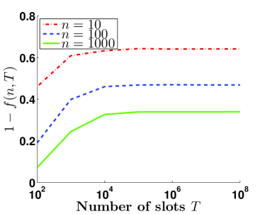
          (b) CSMA/CA

Figure 3: The average percentage of non-empty buffers $1-f(n,T)$ as a function of time $T$ in a random network

From Figure 3.(a) we observe a clear convergence of $1-f(n,T)$; the perhaps surprisingly low limits are conceivably due to the homogeneous transmission probabilities accounting for the bottleneck region. Unlike in the line network, there is a consistent monotonic behavior in the number of nodes $n$, which is likely due to the more uniform structure of the random network setting. In the CSMA/CA case, Figure 3.(b) illustrates that much fewer buffers (by a factor of roughly three) are empty than in the Aloha case, which suggest a less burstier behavior in CSMA/CA.

Clearly, Figures 2 and 3 open several fundamental questions on network queueing behavior for Aloha and CSMA/CA, which may help improving the two. Their main purpose, however, is to convincingly show that the average percentage of non-empty buffers $1-f(n,T)$ is quite small especially in random networks, and in general at small time scales. The key observation is the monotonic (decreasing) behavior (excepting the special Aloha line with $n=10$) in the number of nodes $n$. This behavior is ‘somewhat expected’ in large networks, by invoking laws of large numbers arguments, i.e., the overall incoming and outgoing flows tend to stabilize and thus buffers tend to decrease. This means that both the original upper and lower bounds from Eqs. (2) and (4) become conservative in asymptotic regimes (in $n$). Evidently, this observation is relative to the settings herein herein; whether it generally holds requires further analysis.

In conclusion, the results from this section motivate the need for an analytical approach for network capacity in finite regimes. At this point, we ought to be rigorous in defining capacity in finite time. Concretely, given a time $t$ and an arrival process $D(t)$ at the destination of an e2e path, we are interested in bounds of the form

$$\mathbb{P}\left(D(t)\leq\lambda_{t}t\right)\leq\varepsilon~{},$$

for some violation probability $\varepsilon$. Here, $\lambda_{t}$ is a lower bound on the throughput (capacity) rate of the e2e transmission; upper bounds can be defined similarly by changing the inequality in the probability event.

III A System-Theoretic Approach for Finite Time Capacity

According to the previous discussion, the main challenge to derive capacity results in terms of distributions, and also in finite regimes, is accounting for queueing behavior in a conceivably non-Jackson queueing network. In particular, it is especially hard to analytically keep track of buffer occupancies at relay nodes.

To address this problem, we next describe a general solution to circumvent the characterization of buffer occupancies at the relay nodes, by making an analogy with LTI systems. The idea is to view a single-hop transmission as follows: the data at the source and destination stand for the input and output signals, respectively, whereas the transmission and its characteristics, accounting for both data unavailability due to burstiness or noise due to interference, are modelled by ‘the system’ transforming the input signal; as expected, this system is not linear, but there is a subtle analogy with LTI systems which drives its analytical tractability.

To present the main idea in an approachable manner, from the point of view of notational complexity, we focus on the simplified simple line network from Figure 1; extensions to more involved topologies will be mentioned as well.

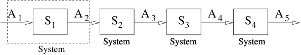
Figure 4: A system interpretation of the multi-hop network from Figure 1

Figure 4 illustrates a system view for the e2e transmission from Figure 1. With abuse of notation the $A_{i}$’s stand for the input/output signals, and the $S_{i}$’s stand for the impulse-responses of the systems. The key property of the impulse-responses is to relate the input and output signals through a convolution operation, i.e.,

$$A_{i+1}=A_{i}*S_{i}~{}.$$ (6)

As it will become more clear in Section IV, the convolution operation denoted here by the symbol ‘$*$’ operates in a $(\textrm{min},+)$ algebra. To be more specific, let $A_{i}$ stand for a stochastic process $A_{i}(t)$, which counts the number of packets in the time interval $[0,t]$ at node $i$; also, let $S_{i}$ stand for (some) bivariate stochastic processes $S_{i}(s,t)$. Then the $(\min,+)$ convolution operation expands as

$$A_{i+1}(t)=\min_{0\leq s\leq t}\left\{A_{i}(s)+S_{i}(s,t)\right\}~{}\forall t\geq 0~{}.$$

The relationship from Eq. (6) has two key properties. One is that it holds for any input signal $A_{i}$, which is hard to derive at relay nodes (when $i\geq 2$). In other words, the impulse-response $S_{i}$ entirely characterizes the system, i.e., the single-hop transmission $i$, which is a key feature of LTI systems since it enables their analytical tractability. The convolution operation has also the useful algebraic property of associativity. The two properties circumvent keeping track of $A_{i}(t)$ at the relay nodes (i.e., for $i=2,3,4$). Indeed, by applying associativity, and using the physical property that the output signal in a system is the input signal at the downstream system, the composition of the four systems from Figure 4 yields the reduced system from Figure 5.

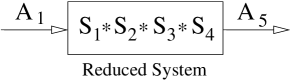
Figure 5: The composition of the four systems from Figure 4 into a single system

The reduced system dispenses with the intermediary signals $A_{2}$, $A_{3}$, and $A_{4}$, and instead it retains the impulse-responses in a composition (or e2e) form, i.e.,

$$A_{5}=A_{1}*\left(S_{1}*S_{2}*S_{3}*S_{4}\right)~{}.$$ (7)

What has yet to be shown concerns the existence of (analytical) expressions for the impulse-responses $S_{i}$’s, satisfying the key property from Eq. (6). The other open issue is whether the convenient reduction from Figure 5 and Eq. (7) is analytically tractable. We will next show that impulse-responses can be constructed for single-hop links in an analogous manner as in LTI systems, depending on the underlying MAC protocol, whereas analytical tractability follows the steps of large deviations or stochastic network calculus theories.

IV Markov Modulated Transmission Processes (MMTPs)

Wireless networks must deal with the fundamental interference problem: two simultaneous transmissions may jointly fail if they interfere with each other. MAC protocols partially resolve this problem by reducing the number of collisions and consequently increasing the network capacity. Obviously, different MAC protocols can lead to different capacities.

To capture the influence of MAC protocols on the throughput capacity, we introduce the concept of Markov Modulated Transmission Process (MMTP). An MMTP is defined for each link, and models the link’s activities (successful/unsuccessful transmissions and idle periods) as a time process and according to the workings of the underlying MAC protocol. The model consists of a Markov chain/process $X(t)$ (depending on the underlying discrete/continuous time model), where $t$ is a time parameter, which modulates the transmission rate of a link $[i\rightarrow j]$, if the source $i$ has data to send at time $t$. In discrete time, the transmission rate in a slot $t$ is

$$S(t-1,t)=C_{X(t)}~{},$$ (8)

where $C_{X(t)}$ is the Markov Modulated Transmission Process defined on the state space ${\mathcal{T}}$ of the Markov chain $X(t)$. It is described as

$$C_{X(t)}=\left\{\begin{array}[]{lll}C&,&X(t)\in{\mathcal{T}}_{[i\rightarrow j]}\\ 0&,&\textrm{otherwise~{},}\end{array}\right.$$ (9)

where ${\mathcal{T}}_{[i\rightarrow j]}\subseteq{\mathcal{T}}$ denotes the set of favorable states of $X(t)$ for the link $[i\rightarrow j]$, which would guarantee a successful transmission if the link has data to send at time $t$; whenever a transmission is successful we assume a constant throughput capacity $C$. The rest of the states $X(t)\in{\mathcal{T}}\backslash{\mathcal{T}}_{[i\rightarrow j]}$ model the times when the link attempts an unsuccessful transmission or it is idle in accordance to the MAC protocol.

The MMTP process $C_{X(t)}$ defined in Eq. (9) is modulated by the Markov chain $X(t)$, and it is conceptually identical with, e.g., Markov Modulated Poisson Processes (MMPPs), which have been used in teletraffic theory to model voice or video (Heffes and Lucantoni [23]). $X(t)$ can be defined either for the whole network (when it modulates the transmission opportunities of all the links) or for each link separately. In turn, $C_{X(t)}$ is always separately defined for each link.

We point out that the process $S(s,t)$, which we loosely introduced in Eq. (8) through its increments $S(t-1,t)$, directly corresponds to the impulse-response process introduced in Section III to entirely characterize the behavior of a single-hop transmission in system theoretic terms (see Figure 4 and Eq. (6)). We mention that the impulse-response defined in Eq. (8) corresponds to the effective capacity concept proposed by Wu and Negi in [35] to model the instantaneous channel capacity. This concept was used by Tang and Zhang [34] to analyze the impact of physical layer characteristics (e.g., MIMO) on delay at the data-link layer. The MMTP idea was also used explicitly by Fidler [18], Mahmood et al. [28], Al-Zubaidy et al. [38], Zheng et al. [37] and implicitly by Ciucu et al. [9, 8], to model channel service processes with Markov chains. Relative to these previous works, our contribution herein is to fit the effective capacity concept, defined as a Markov modulated process, for three specific MAC protocols in the framework of the stochastic network calculus. A key feature of network calculus is that it facilitates the analysis of network queueing problems by relying on a subtle analogy with LTI systems (see Le Boudec and Thiran [5], and Ciucu and Schmitt [12]).

In the following we explicitly construct the impulse-response process $S(s,t)$, and the underlying Markov process $X(t)$ and MMTP $C_{X(t)}$, for three MAC protocols. In addition, we outline the key steps to compute the (per-flow) distribution of the throughput capacity in closed-form.

IV-A Centralized scheduling

Assuming a time-slotted model and the nodes’ perfect synchronization, the idea of centralized scheduling is to pre-allocate the transmission slots to the nodes in order to avoid collisions. In unsaturated scenarios, an optimal solution (i.e., attaining maximal throughput) would require significant overhead as the centralized scheduler would require keeping track of the arrival processes at each of the nodes. Even in saturation scenarios, the optimality problem is in fact NP-complete in general networks (see, e.g., Sharma et al. [32]).

For the network model from Figure 1.(a-b), the optimal scheduling allocation starting from slot $1$, in terms of links, is: $\{1,2,3,(1,4),2,3,(1,4),\dots\}$; for instance, link $2$ is allocated the slots $2,5,8,\dots$ That means that link $2$ is given full transmission capacity (say $C$) during these slots, which suggests that the bivariate function

$$S_{2}(s,t)=C\sum_{u=s+1}^{t}I_{(u-2)\%3=0}~{}\forall 2\leq s\leq t~{},$$ (10)

and $0$ everywhere else, characterizes the capacity of link $2$ in terms of the $(\textrm{min},+)$ convolution from Eq. (6) ($I_{E}$ denotes the indicator function taking the values $0$ and $1$, depending on whether the event $E$ is false or true). The intuition is that $S_{2}(s,t)$ counts the number of packets transmitted over link $2$ in the time interval $(s,t]$, if node $2$ is saturated.

This saturation condition translates into system theoretic terms as follows: the input signal to the second system in Figure 4 is the infinite signal $A_{2}(t)=\infty$ for $\forall t$ (also called the impulse), whereas the corresponding output, i.e., the impulse-response, is the signal $S_{2}(t)$, or $S_{2}(0,t)$ in the notation from Eq. (10). Therefore, the construction of $S_{2}(s,t)$ is analogous to the construction of impulse-response functions in LTI systems, which are the output from an LTI system with input given by the Kronecker signal (see [26]). Although the system representing the link’s transmission is not linear, even under the $(\min,+)$ algebra, the constructed process $S_{2}(s,t)$ entirely characterizes link $2$, i.e.,

$$A_{3}(t)=\min_{0\leq s\leq t}\left\{A_{2}(s)+S_{2}(s,t)\right\}~{}\forall t\geq 0~{},$$ (11)

for all $A_{2}(t)$ at the input of the second system.

So far we directly constructed $S_{2}(s,t)$ without resorting on an MMTP $C_{X(t)}$. The underlying MMTP, and also the modulating Markov chain $X(t)$, are depicted in Figure 6.(a). The states of $X(t)$ denote the set of transmitting links (according to the centralized schedule). The transition probabilities between the states are all equal to $1$, thus reflecting the deterministic nature of centralized scheduling. The MMTP process for link $[A_{2}\rightarrow A_{3}]$ is

$$C_{X(t)}=\left\{\begin{array}[]{lll}C&,&\textrm{if}~{}X(t)=\left\{2\right\}\\ 0&,&\textrm{otherwise~{}.}\end{array}\right.$$

The MMTPs for the other links are defined similarly; for instance, for links $1$ and $4$, the only change is that $C_{X(t)}=C$ when $X(t)=\left\{1,4\right\}$. Note that all MMTPs share the same Markov chain modulating the transmission opportunities at the network level. Moreover, $X(t)$ and $C_{X(t)}$ jointly reproduce the expressions of the impulse responses (e.g., of $S_{2}(s,t)$ from Eq. (10)) according to the definition from Eq. (8).

Concerning analytical tractability, we remark that the reduced system from Figure 5 is implicitly tractable since the constructed impulse-responses $S_{i}(s,t)$ are deterministic functions. The overall impulse-response of the e2e path $S=S_{1}*S_{2}*S_{3}*S_{4}$ from Eq. (7) can be computed directly, i.e.,

$$S(s,t)=C\sum_{u=s+1}^{t}I_{(u-1)\%3=0}~{}\forall 1\leq s\leq t~{},$$ (12)

and $0$ everywhere else. To quickly check how the e2e impulse-response $S$ captures the causality condition, assume that $A_{1}(1)=1$ (i.e., one packet arrives at time $1$). Then this packet departs the network no sooner than at time $4$: indeed, $A_{5}(3)=A_{1}*S(3)=0$, as $S(0,3)=0$, and that $A_{5}(4)=\min_{0\leq s\leq 4}\left\{A_{1}(s)+S(s,4)\right\}=1$, with the minimum being attained at $s=0$.

Although the constructions of the MMTP’s above is not technically necessary, as the impulse-responses were directly constructed, and the impulse-response $S(s,t)$ of the e2e path could be in principle determined by other means than computing an e2e convolution, we regard this detour to be insightful for the construction of impulse-responses for the more challenging cases of Aloha and CSMA/CA protocols.

(a) Centralized scheduling

                                             (b) Aloha

Figure 6: Markov Modulated Transmission Processes (MMTPs) for link $[A_{2}\rightarrow A_{3}]$

IV-B Aloha

The slotted-Aloha MAC protocol (called Aloha here) is an elegant solution to circumvent centralized scheduling (see Ambramson [1]). The key idea is that each node attempts to transmit with some probability in each time slot and when data is available; a transmission $[i\rightarrow j]$ is successful in some time slot $t$ if $i$ is the only node in the interference range of node $j$ attempting to transmit in that slot. While the protocol is entirely distributed, it may experience significant performance decay, e.g., the achieved capacity can be as small as $36\%$ of the theoretical limit.

To construct the impulse-response processes for the line network from Figure 1.(a-b), we first construct the MMTP processes. We focus again on link $[A_{2}\rightarrow A_{3}]$. The underlying MMTP, and also the modulating Markov chain $X(t)$, are depicted in Figure 6.(b). The meaning of state ‘on’ is that, while $X(t)$ delves in it, the relay node $A_{2}$ successfully transmits (if there is data to send). In turn, while $X(t)$ delves in state ‘off’, $A_{2}$ is either idle (in accordance with the workings of Aloha) or it is involved in a collision. Assuming, for convenience, that all nodes transmit with the same probability $p$, the transition probabilities are $\pi_{1}=p(1-p)^{3}$ and $\pi_{2}=1-\pi_{1}$ (the power of $3$ is the degree of node $2$ in the contention graph from Figure 1.(b)). For this Markov chain, the steady-state probabilities are $\pi_{\textrm{on}}=\pi_{1}$ and $\pi_{\textrm{off}}=\pi_{2}$, and $X(t)$ has the convenient property of statistically independent increments, e.g., $\forall t$

$$\mathbb{P}\left(X(t+1)=\textrm{`on'}|X(t)=\textrm{`off'}\right)=\mathbb{P}\left(X(t+1)=\textrm{`on'}\right)~{}.$$ (13)

The definition of the associated MMTP should be intuitive at this point, i.e.,

$$C_{X(t)}=\left\{\begin{array}[]{lll}C&,&\textrm{if}~{}X(t)=\textrm{`on'}\\ 0&,&\textrm{otherwise~{},}\end{array}\right.$$ (14)

as also illustrated in Figure 6.(b). In other words, $A_{2}$ can successfully transmit (assuming it has data) at full rate $C$ while the modulating process $X(t)$ delves in the favorable state ‘on’.

The construction of the other links’ MMTP processes is almost identical, except for the transmission probabilities of the modulating process. For instance, for the links $[A_{1}\rightarrow A_{2}]$ and $[A_{4}\rightarrow A_{5}]$, the new transmission probabilities are $\pi_{1}=p(1-p)^{2}$ and $\pi_{2}=1-\pi_{1}$ (the power of $2$ is the common degree of nodes $1$ and $4$ in the contention graph from Figure 1.(b)).

These MMTP processes directly determine the impulse-response functions $S_{i}(s,t)$, corresponding to the single-hop links $i=1,2,3,4$, according to the definition from Eq. (8). Furthermore, the composition property of the $S_{i}(s,t)$’s in the underlying $(\min,+)$ algebra lends itself to the entire characterization of the throughput capacity over the e2e path as in Eq. (7), i.e.,

$$A_{5}=A_{1}*S~{},$$

where $S=S_{1}*S_{2}*S_{3}*S_{4}$ is the impulse-response of the e2e path.

Unlike centralized scheduling which may lend itself to an explicit expression for $S$ (e.g., as in Eq. (12)), Aloha is conceivably more challenging with respect to the analytical tractability of the reduced system. One immediate issue lies in the probabilistic structure of the local impulse-responses $S_{i}$’s. A more subtle issue lies in the fact that the $S_{i}$’s are statistically correlated random processes, even in the simplified line network.

To deal with these challenges, the key idea is to trade analytical exactness for tractability. More concretely, instead of exactly deriving the e2e transient capacity in closed-form (an open problem in itself), we compute bounds by relying on large deviation techniques (e.g., as in [9]). Let us illustrate such computations for the first two hops only, and a saturation assumption at node $A_{1}$ (the relay nodes are however not assumed to be saturated). The probability of violating a lower bound $\lambda_{t}$, on the transient throughput rate over the time scale $[0,t]$, can be computed as follows for some $\theta>0$

$$\mathbb{P}\left(A_{3}(t)\leq\lambda_{t}t\right)=\mathbb{P}\left(S_{1}*S_{2}(t)\leq\lambda_{t}t\right)$$ (15)

$$=\mathbb{P}\left(\sup_{0\leq s\leq t}\left\{\lambda_{t}t-S_{1}(s)-S_{2}(s,t)\right\}\geq 0\right)$$

$$\leq\sum_{0\leq s\leq t}e^{\theta\lambda_{t}t}E\left[e^{-\theta S_{1}(s)}\right]E\left[e^{-\theta S_{2}(s,t)}\right]~{},$$

by using Boole’s inequality and the Chernoff bound; in the first line we also used the saturation assumption at mode $A_{1}$, e.g., $A_{1}(1)=\infty$. The last step is also based on the statistical independence between the impulse-responses $S_{1}(u,s)$ and $S_{2}(s,t)$ (in order to apply $E[XY]=E[X]E[Y]$ for some independent r.v.’s $X$ and $Y$); this holds because $(u,s]$ and $(s,t]$ are non-overlapping intervals, whereas the corresponding Markov modulated processes of $S_{1}(u,s)$ and $S_{2}(s,t)$ have statistically independent increments (recall the convenient property from Eq. (13)). Therefore, although $S_{1}(u,s)$ and $S_{2}(u,s)$ are correlated over overlapping intervals, the expansion of the $(\min,+)$ convolution (in terms of non-overlapping intervals) and the independent increments property from Eq. (13) justify the last step.

The Laplace transforms in the last equation can be computed explicitly for the impulse-responses. Concretely, one has $E\left[e^{-\theta S_{i}(s,t)}\right]\leq e^{-\theta r_{s}(t-s)}$, where $r_{s}=\frac{\log{\left(qe^{-\theta C}+1-q\right)^{-1}}}{\theta}$ and $q=p(1-p)^{2}$. Evaluating the nested sums from Eq. (15) yields the following closed-form bound

$$\mathbb{P}\left(A_{3}(t)\leq\lambda_{t}t\right)\leq\inf_{\theta}(t+1)e^{-\theta(r_{s}-\lambda_{t})t}~{}.$$ (16)

The result is not explicit, as $\theta$ is to be optimized (typically numerically). Setting the right-hand side to some violation probability, the lower bound $\lambda_{t}$ on the transient capacity rate follows immediately. We mention that probabilistic upper bounds can also be derived similarly by a sign change in Eq. (15); moreover, the case of non-saturated arrivals $A_{1}(t)$ follows similarly by plugging-in their moment generating function (see [8]).

Next we give a general result for computing the upper and lower bounds on the end-to-end throughput capacity for a flow crossing $k$ hops.

Theorem 1

(Capacity Bounds (Upper and Lower Bounds) - Aloha) Consider a flow crossing $k$ hops. Assume that the impulse-response process $S_{j}(s,t)$, at each hop $j$, satisfies the following bounds on the MGF and Laplace transforms: $E\left[e^{\theta S_{j}(s,t)}\right]\leq e^{\theta r_{j}(\theta)(t-s)}$ and $E\left[e^{-\theta S_{j}(s,t)}\right]\leq e^{-\theta r_{j}(-\theta)(t-s)}$ for all $\theta>0$. Let $r(\theta)=\max_{j}r_{j}(\theta)$ and $r(-\theta)=\min_{j}r_{j}(-\theta)$. Assume also that $S_{j}(s,t)$ are statistically independent over non-overlapping intervals. Then, for some $\varepsilon>0$, a probabilistic lower bound on the capacity rate is for all $t\geq 0$

$$\lambda_{t}^{L}=\sup_{\theta>0}\left\{r(-\theta)+\frac{\log{\varepsilon}-\log{\binom{t+k-1}{k-1}}}{\theta t}\right\}~{},$$ (17)

The corresponding upper bound is

$$\lambda^{U}_{t}=\inf_{\theta>0}\left\{r(\theta)-\frac{\log{\varepsilon}}{\theta t}\right\}~{}.$$ (18)

Proof. Denote $A(t)$ and $D(t)$ the arrival and departure processes of the flow at the first node and last node, respectively; assume the saturated condition that $A(t)=\infty$. Applying the end-to-end service curve from Eq. (7), extended to $k$ hops, we can write

$$\mathbb{P}\left(D(t)\leq\lambda_{t}^{L}t\right) \leq \mathbb{P}\left(A*S(t)\leq\lambda_{t}^{L}t\right)$$

$$= \mathbb{P}\left(S_{1}*S_{2}*\dots*S(t)\leq\lambda_{t}^{L}t\right)~{}.$$

Letting $u_{0}=0$ and $u_{k}=t$ we can continue bound the probability using the Chernoff bound:

$$\mathbb{P}\left(\inf_{0\leq u_{1}\leq\dots\leq u_{k-1}\leq t}\sum_{j=1}^{k}S_{j}\left(u_{j-1},u_{j}\right)\leq\lambda_{t}^{L}t\right)$$

$$\leq\sum_{u_{0}\leq\dots\leq u_{k}}\prod_{j=1}^{k}E\left[{}^{-\theta S_{j}(u_{j-1},u_{j})}\right]e^{\theta\lambda_{t}^{L}t}$$

$$\leq\sum_{0\leq u_{1}\leq\dots\leq u_{k}}\prod_{j=1}^{k}e^{-\theta r_{j}(-\theta)(u_{j}-u_{j-1})}e^{\theta\lambda_{t}^{L}t}$$

$$=\binom{t+k-1}{k-1}e^{-\theta\left(r(-\theta)-\lambda_{t}^{L}\right)t}~{},$$

where the binomial term is the number of combinations with repetition. Equalizing the last term to $\varepsilon$ gives the bound $\lambda_{t}^{L}$.

In turn, for the upper bound, we can write

$$\mathbb{P}\left(D(t)\geq\lambda^{U}_{t}t\right)=\mathbb{P}\left(A*S(t)\geq\lambda^{U}_{t}t\right)$$

$$=\mathbb{P}\left(S_{1}*S_{2}*\dots*S(t)\geq\lambda^{U}_{t}t\right)$$

$$\leq\inf_{u_{1}\leq\dots\leq u_{k}}\mathbb{P}\left(\sum_{j=1}^{k}S_{j}(u_{j-1},u_{j})\geq\lambda^{U}_{t}t\right)$$

$$\leq\inf_{u_{1}\leq\dots\leq u_{k}}\prod_{j=1}^{k}E\left[{}^{\theta S_{j}(u_{j-1},u_{j})}\right]e^{-\theta\lambda_{t}^{U}t}$$

$$\leq e^{-\theta\left(\lambda_{t}^{U}-r(\theta)\right)t}~{}.$$

Equalizing the obtained bound with $\varepsilon$ and solving for $\lambda^{U}_{t}$ we obtain the value from Eq. (18), which completes the proof.  $\Box$

IV-C CSMA/CA

The CSMA/CA protocol was motivated by the need to increase the (very) low capacity of Aloha, while preserving the distributive aspect of the protocol. One key idea is to prevent collisions from happening by enabling nodes to ‘listen to the channel’ before transmitting. The other key idea is that once a node perceives the channel as being busy, the node enters in an exponentially distributed backoff mode.

We use a simplified CSMA/CA protocol, developed by Durvy et al. [15], which retains the key features of CSMA/CA. For the network from Figure 1.(a-b), the construction of the MMTP processes, and also of the impulse-response processes $S_{i}(s,t)$, follows similarly as for centralized scheduling and Aloha. For the link $[A_{2}\rightarrow A_{3}]$, the underlying MMTP, and also the modulating (now continuous-time) Markov process $X(t)$, are depicted in Figure 7. $X(t)$ is constructed exactly as in [15], where $\nu^{-1}$ and $\mu^{-1}$ denote the average backoff and transmission times. The interpretation of the states is identical as for centralized scheduling (see Figure 6.(a)); while $X(t)$ delves in the new state $\{0\}$, all nodes are in a backoff mode. Ignoring the details of switching from discrete to continuous time, the MMTP is defined as for Aloha (see Eq. (14)), i.e.,

Figure 7: A Markov Modulated Transmission Process (MMTP) for link $[A_{2}\rightarrow A_{3}]$

$$C_{X(t)}=\left\{\begin{array}[]{lll}C&,&\textrm{if}~{}X(t)=\textrm{\{2\}}\\ 0&,&\textrm{otherwise~{},}\end{array}\right.$$

and the impulse-response $S_{2}(s,t)$ is defined as in Eq. (8). The MMTPs for the other links are defined similarly (e.g., for $[A_{1}\rightarrow A_{2}]$, the only change is that $C_{X(t)}=C$ when $X(t)\in\left\{\{1\},\{1,4\}\right\}$).

Unlike Aloha, CSMA/CA is subject to more compounded calculations of the e2e throughput capacity. Note that the first two lines from Eq. (15) still hold. The last line, however, does not hold anymore since $S_{1}(u,s)$ and $S_{2}(s,t)$ are not statistically independent, even over non-overlapping intervals. The reason lies in the Markov modulating process $X(t)$ which does not have independent increments (as in Eq. (13) for Aloha). The immediate solution is to apply Hölder’s inequality to bound $E\left[e^{-\theta S_{1}(s)}e^{-\theta S_{2}(s,t)}\right]$, as suggested for the Aloha case in extended (not-necessarily line) networks.

The last unaddressed issue concerns the computation of the Laplace transforms for the impulse-responses $S_{i}(s,t)$’s. Since these processes are Markov arrival processes (MAPs), their Laplace transforms can be computed using standard techniques from teletraffic theory (see Courcoubetis and Weber [13]). Let us briefly reproduce such techniques and compute in particular

$$L_{2,t}:=E\left[e^{-\theta S_{2}(t)}\right]~{},$$

for some $\theta>0$. Denote the six states of the MAP from Figure 7 by the numbers $1,2,\dots,6$, and the elements of the generator matrix $P$ by $p_{i,j}$, i.e.,

$$P=\left(\begin{array}[]{cccccc}-4\nu&\nu&\nu&\nu&\nu&0\\ \mu&-(\mu+\nu)&0&0&0&\nu\\ \mu&0&-\mu&0&0&0\\ \mu&0&0&-\mu&0&0\\ \mu&0&0&0&-(\mu+\nu)&\nu\\ 0&\mu&0&0&\mu&-2\mu\end{array}\right)~{}.$$

Denote also the conditional Laplace transforms $L_{2,i,t}:=E\left[e^{-\theta S_{2}(t)}\mid X(0)=i\right]$, i.e., conditioned on the initial state of the Markov chain $X(t)$, which is assumed to start in steady-state. For some initial state (e.g., $i=3$) we have the backward equation

$$L_{2,3,t+\Delta t} = E\left[e^{-\theta S_{2}(\Delta t)}\mid X(0)=3\right]$$

$$\qquad\sum_{j}E\left[e^{-\theta S_{2}(\Delta t,t+\Delta t)}\mid X(\Delta t)=j\right]p_{3,j}$$

$$= e^{-\theta C\Delta t}\left(L_{2,0,t}\mu\Delta t+L_{2,3,t}\left(1-\mu\Delta t\right)+o(\Delta t)\right)~{},$$

where $\lim_{\Delta t\rightarrow 0}\frac{o(\Delta t)}{\Delta t}=0$. In the last line we used the stationarity of $S_{2}(t)$. Using the Taylor’s expansion $e^{-\theta C\Delta t}=1-\theta C\Delta t+o(\Delta t)$, rearranging terms, and taking the limit $\Delta t\rightarrow 0$ it follows that

$$\frac{\partial L_{2,3,t}}{\partial t}=L_{2,0,t}\mu-L_{2,3,t}(\mu+\theta C)~{}.$$ (19)

One can proceed similarly to derive the PDE’s of the other $L_{2,i,t}$’s for $i\neq 3$, and arrive at the system of PDE’s

$$\frac{\partial\mbox{\boldmath${L_{2,t}}$}}{\partial\mbox{\boldmath${t}$}}=B_{2}\mbox{\boldmath${L_{2,t}}$}~{},$$ (20)

where $\mbox{\boldmath${L_{2,t}}$}=(L_{2,1,t},\dots,L_{2,6,t})^{T}$ and $B_{2}$ is a matrix whose lines are formed according to Eq. (19), i.e.,

$$B_{2}=\left(\begin{array}[]{cccccc}-4\nu&\nu&\nu&\nu&\nu&0\\ \mu&-(\mu+\nu)&0&0&0&\nu\\ \mu&0&-(\mu+\theta C)&0&0&0\\ \mu&0&0&-\mu&0&0\\ \mu&0&0&0&-(\mu+\nu)&\nu\\ 0&\mu&0&0&\mu&-2\mu\end{array}\right)~{}.$$

Note that $B_{2}$ differ from the generator matrix $P$ by the term $-\mu C$ on the position $(3,3)$, which is due to the transmission at rate $C$ while in state $3$ (i.e., the state labelled ‘$\{2\}$’ from Figure 7). Solving for Eq. (20) we get the solution

$$\mbox{\boldmath${L_{2,t}}$}=\sum_{i=1}^{6}c_{i}e^{\lambda_{i}t}\mbox{\boldmath${x_{i}}$}~{},$$

where $\lambda_{i}$ and ${x_{i}}$ are the eigenvalues and eigenvectors, respectively, of the matrix $B_{2}$. The coefficients $\mbox{\boldmath${c}$}=\left(c_{1},\dots,c_{n}\right)^{T}$ can be determined from the initial condition $\mbox{\boldmath${c}$}=X^{-1}\mbox{\boldmath${1}$}$, $X=\left(\mbox{\boldmath${x_{1}}$},\dots,\mbox{\boldmath${x_{n}}$}\right)$ and $\mbox{\boldmath${1}$}=\left(1,\dots,1\right)^{T}$. Because the modulating process starts in the steady-state, we obtain the solution of the Laplace transform $L_{2,t}=\sum_{i=1}^{6}\pi_{i}L_{2,i,t}$. This takes the hyperexponential form

$$L_{2,t}=E\left[e^{-\theta S_{2}(t)}\right]=\sum_{i=1}^{6}L_{2,i}e^{\lambda_{i}t}~{},$$ (21)

where $L_{2,i}=c_{i}\sum_{j}\pi_{j}X_{j,i}$. Since $\sum_{i}L_{2,i}=1$, we have the simplified bound

$$E\left[e^{-\theta S_{2}(t)}\right]\leq e^{\lambda_{6}t}~{},$$ (22)

where, by convention, $\lambda_{6}=\max_{i}\lambda_{i}$ is the spectral radius of the matrix $B_{2}$.

The other Laplace transforms can be computed similarly, by suitably modifying the MMTP as mentioned earlier. The only difference, when computing $E\left[e^{-\theta S_{j}(t)}\right]$, is that the corresponding matrix $B_{j}$ is given by

$$B_{j}=P-\theta CI_{j}$$ (23)

where $I_{j,i,i}=1$ if there is a transmission at rate $C$ in the corresponding MMTP, and $I_{j,i,l}=0$ otherwise (as an example, when $j=4$, then $I_{j,5,5}=1$, $I_{j,6,6}=1$, and $I_{j,i,l}=0$ otherwise).

Compared to Aloha, the drawback of the closed-form results obtained for CSMA/CA is that they depend on the eigenvalues/eigenvectors of the matrix $B$ (appearing in the solution of Eq. (20)), and are thus not easily amenable to convex optimizations. The next theorem extends Theorem 1 to the CSMA/CA case.

Theorem 2

(Capacity Bounds (Upper and Lower Bounds) - CSMA/CA) Consider a flow crossing $k$ hops and the corresponding MMTP being modulated by a generator matrix $P$. For $j=1,2,\dots,k$, let $\lambda_{j}$ as the spectral radiuses of the matrixes $B_{j}$ constructed as in Eq. (23) with $\theta$ replaced by $k\theta$. Let $r_{j}(-k\theta):=\frac{\lambda_{j}}{-k\theta}$ and $r(-k\theta)=\min_{j}r_{j}(-k\theta)$. Then, for some $\varepsilon>0$, a probabilistic lower bound on the capacity rate is for all $t\geq 0$

$$\lambda_{t}^{L}=\sup_{\theta>0}\left\{r(-k\theta)+\frac{\log{\varepsilon}-\log{\binom{t+k-1}{k-1}}}{\theta t}\right\}~{},$$ (24)

In turn, for the upper bound, let $\lambda_{j}$ as the spectral radiuses of the matrixes $B_{j}$ constructed as in Eq. (23) with $\theta$ replaced by $-k\theta$, for $j=1,2,\dots,k$. Let also $r_{j}(k\theta):=\frac{\lambda_{j}}{k\theta}$ and $r(k\theta)=\max_{j}r_{j}(k\theta)$. Then, for some $\varepsilon>0$, a probabilistic upper bound on the capacity rate is for all $t\geq 0$

$$\lambda^{U}_{t}=\inf_{\theta>0}\left\{r(k\theta)-\frac{\log{\varepsilon}}{\theta t}\right\}~{}.$$ (25)

Proof. The proof proceed similarly as the proof of Theorem 1, with the observation that one has to account for the fact that the impulse-responses $S_{j}(s,t)$ are not anymore statistically independent (even over non-overlapping intervals).

The first step is identical, i.e.,

$$\mathbb{P}\left(D(t)\leq\lambda_{t}^{L}t\right) \leq \mathbb{P}\left(A*S(t)\leq\lambda_{t}^{L}t\right)$$

$$= \mathbb{P}\left(S_{1}*S_{2}*\dots*S(t)\leq\lambda_{t}^{L}t\right)~{}.$$

For the second step, we additionally rely on Hölder’s inequality:

$$\mathbb{P}\left(\inf_{0\leq u_{1}\leq\dots\leq u_{k-1}\leq t}\sum_{j=1}^{k}S_{j}\left(u_{j-1},u_{j}\right)\leq\lambda_{t}^{L}t\right)$$

$$\leq\sum_{u_{0}\leq\dots\leq u_{k}}\prod_{j=1}^{k}\left(E\left[{}^{-k\theta S_{j}(u_{j-1},u_{j})}\right]\right)^{\frac{1}{k}}e^{\theta\lambda_{t}^{L}t}$$

$$\leq\sum_{0\leq u_{1}\leq\dots\leq u_{k}}\prod_{j=1}^{k}e^{-\theta r_{j}(-k\theta)(u_{j}-u_{j-1})}e^{\theta\lambda_{t}^{L}t}$$

$$=\binom{t+k-1}{k-1}e^{-\theta\left(r(-k\theta)-\lambda_{t}^{L}\right)t}~{},$$

where the binomial term is the number of combinations with repetition. Equalizing the last term to $\varepsilon$ gives the bound $\lambda_{t}^{L}$.

In turn, for the upper bound, we can write

$$\mathbb{P}\left(D(t)\geq\lambda^{U}_{t}t\right)=\mathbb{P}\left(A*S(t)\geq\lambda^{U}_{t}t\right)$$

$$=\mathbb{P}\left(S_{1}*S_{2}*\dots*S(t)\geq\lambda^{U}_{t}t\right)$$

$$\leq\inf_{u_{1}\leq\dots\leq u_{k}}\mathbb{P}\left(\sum_{j=1}^{k}S_{j}(u_{j-1},u_{j})\geq\lambda^{U}_{t}t\right)$$

$$\leq\inf_{u_{1}\leq\dots\leq u_{k}}\prod_{j=1}^{k}\left(E\left[{}^{k\theta S_{j}(u_{j-1},u_{j})}\right]\right)^{\frac{1}{k}}e^{-\theta\lambda_{t}^{U}t}$$

$$\leq e^{-\theta\left(\lambda_{t}^{U}-r(k\theta)\right)t}~{}.$$

Equalizing the obtained bound with $\varepsilon$ and solving for $\lambda^{U}_{t}$ we obtain the value from Eq. (25), which completes the proof.  $\Box$

En passant, we point out that existing multi-hop results (especially for CSMA MACs) rely on independence assumptions across hops (e.g, [20, 36]), in addition to the saturation assumption at the relay nodes. In fact, even the seminal single-hop result obtained by Bianchi [3] relies on the artificial assumption that nodes independently see the system in the steady-state. We raise the awareness that convenient statistical assumptions are inherently prone to incorrect results, even when given as asymptotic scaling laws, as long as independence assumptions extend over a number of hops as a function of the total number of hops. This pitfall has been also pointed out even in an M/M/1 packet tandem network (wired), subject to the classical Kleinrock’s independence assumption (see [6]).

V Application: Single-Hop vs. Multi-Hop

In this section we give an illustrative example on using the finite time and space key features of our capacity bounds for the following problem. Consider the network from Figure 8 with $k+1$ nodes, all in the interference range of each other, and all being saturated and attempting to access the channel using either the Aloha or CSMA/CA protocols. Given that node $A_{1}$ intends to transmit to node $A_{k+1}$, the problem concerns choosing between the following two routing strategies:

1. Single-hop: Node $A_{1}$ directly transmits to node $A_{k+1}$ at rate $r_{\textrm{sh}}$.

2. Multi-hop: Node $A_{1}$ transmits using the nodes $A_{2},~{}A_{3},\dots,A_{k}$ as relays; the rate for each transmission $\left[A_{j}\rightarrow A_{j+1}\right]$ is $r_{\textrm{mh}}$.

In order to avoid a trivial answer we assume that $r_{\textrm{sh}}<r_{\textrm{mh}}$.

(a) Single-hop

(b) Multi-hop

Figure 8: Which strategy should node $A_{1}$ choose in order to transmit to $A_{k+1}$? (all nodes hear each other, all are saturated, and $r_{\textrm{sh}}<r_{\textrm{mh}}$)

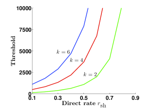
(a) Aloha

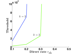
(b) CSMA/CA

Figure 9: The time scale (threshold) after which the multi-hop is more advantageous than the single-hop strategy ($\varepsilon=10^{-3}$, normalized per-hop rate $r_{\textrm{mh}}=1$, variable direct rate $r_{\textrm{sh}}$, Aloha transmission probability $p=\frac{1}{k}$, and $\nu=\mu=0.1$ for CSMA/CA)

Figure 9 illustrates the threshold at which the multi-hop strategy is more advantageous. More concretely, the values displayed (i.e., the ‘Threshold’) are the time scales at which the lower-bound for the multi-hop transmission is larger than the upper-bound for the single-hop transmission. Both (a) and (b) indicate the intuitive facts that the ‘Threshold’ is exponential in the relative direct rate $r_{\textrm{sh}}$ and also increasing in the number of hops $k$. In (b), for CSMA/CA, the benefits of multi-hop routing hold only for very low relative direct rate $r_{\textrm{sh}}$ and quickly vanish by increasing $k$. We point out however that this quick blow-up may be due to the loose underlying upper bounds on the CSMA/CA per-flow capacity. In the case of Aloha, however, both the lower and upper bounds are reasonably tight. For actual illustrations of the numerical tightness of the bounds we refer to Section VI.

The above routing problem has been debated in different settings such as wireless mesh and sensor networks. Experimental results by De Couto et al. [14] showed that minimizing the hop count is not always the best option as long hops may incur a high packet error rate. Jain et al. [24] showed that, due to interference, shortest paths with long hops may not provide the best performance. In contrast, there are several results supporting long-hop routing. Haenggi and Puccinelli [22] provided many reasons why short-hop routing is not as beneficial as it seems to be. Moreover, in energy limited networks such as sensor networks, long-hop routing may also be preferable (see Ephremides [16] and Björnemo et al. [4]).

Our contribution to this debate is to bring a new perspective on single vs. multi-hop routing by focusing on the underlying time scale. Concretely, we provided theoretical evidence that multi-hop routing is more advantageous in the long-run for Aloha. In turn, in the case of CSMA/CA, the advantage of multi-hop vanishes in most cases. We raise however the awareness that, for the purpose of analytical tractability, our results are restricted to a line network and no frequency or power management being accounted for.

VI Numerical Results

Here we briefly illustrate the numerical tightness of the derived lower and upper bounds on the transient throughput rate from Theorems 1 and 2. We consider the network from Figure 8.(b) in which node $A_{1}$ transmits to node $A_{k+1}$ in a multi-hop fashion. We use the parameters per-hop rate $r_{\textrm{mh}}=1$, $p=\frac{1}{k}$ for Aloha, $\frac{1}{\nu}=\frac{1}{\mu}=10$ for CSMA/CA, and a violation probability $\varepsilon=10^{-3}$.

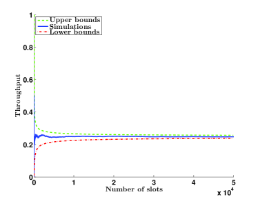
(a) Aloha, $k=2$

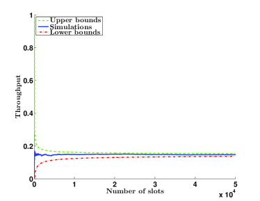
(b) Aloha, $k=3$

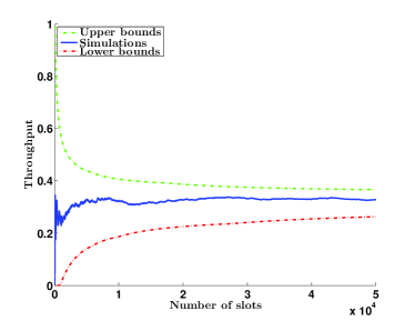
(c) CSMA/CA, $k=2$

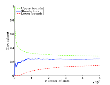
(d) CSMA/CA, $k=3$

Figure 10: Throughput rates as a function of the number of time slots.

Figure 10 indicates that the upper and lower bounds for Aloha are quite tight. For CSMA/CA, however, only the upper bounds remain reasonably tight whereas the lower bounds tend to degrade with the number of hops $k$. This is due to the underlying application of the Boole’s inequality, which is known to be loose in the case of correlated arrivals (see, e.g., [10]).

VII Conclusions

We have presented the key ingredients of a unified system-theoretic methodology to compute the per-flow capacity in finite time and space network scenarios, and for three MAC protocols: centralized scheduling, Aloha, and CSMA/CA. We have also confirmed the anecdotal practical conservative nature of alternative asymptotic results, by closely analyzing a widely used double-limit argument. Moreover, we have demonstrated that our finite time/space results can lend themselves to engineering insight, i.e., on the time scales at which multi-hop routing becomes more advantageous than single-hop routing.

The presented methodology faced however the following dilemma concerning analytical tractability vs. the level of modelling details. One one hand, we have managed to employ a rigorous mathematical analysis. On the other hand, due to the hardness of dealing with spatio-temporal correlations in non-Jackson queueing networks, we have restricted to a line network and simplified MAC protocols, while ignoring physical layer considerations. Moreover, we have employed bounding techniques from the effective bandwidth literature, and whose numerical accuracy is problematic in the case of correlated processes (e.g., Choudhury et al. [7]). While such techniques produced good estimates for the Aloha case, there is a need for advanced techniques to properly account for the underlying correlations in CSMA/CA. Nevertheless we believe that the advocated system-theoretic approach has the potential to contribute to the development of the long desirable functional network information theory (see Andrews et al. [2]).

References

- [1] N. Abramson. The Aloha system: another alternative for computer communications. In Proceedings of AFIPS Joint Computer Conferences, pages 281–285, 1970.
- [2] J. G. Andrews, N. Jindal, M. Haenggi, R. Berry, S. Jafar, D. Guo, S. Shakkottai, R. Heath, M. Neely, S. Weber, and A. Yener. Rethinking Information Theory for mobile ad hoc networks. IEEE Communications Magazine, 46(12):94–101, Dec. 2008.
- [3] G. Bianchi. Performance analysis of the IEEE 802.11 distributed coordination function. IEEE Journal on Selected Areas in Communications, 18(3):535–547, Mar. 2000.
- [4] E. Björnemo, M. Johansson, and A. Ahlén. Two hops is one too many in an energy-limited wireless sensor network. In IEEE International Conference on Acoustics, Speech and Signal Processing, 2007.
- [5] J.-Y. Le Boudec and P. Thiran. Network Calculus. Springer Verlag, Lecture Notes in Computer Science, LNCS 2050, 2001.
- [6] A. Burchard, J. Liebeherr, and F. Ciucu. On superlinear scaling of network delays. IEEE/ACM Transactions on Networking, 19(4):1043–1056, Aug. 2011.
- [7] G. Choudhury, D. Lucantoni, and W. Whitt. Squeezing the most out of ATM. IEEE Transactions on Communications, 44(2):203–217, Feb. 1996.
- [8] F. Ciucu. On the scaling of non-asymptotic capacity in multi-access networks with bursty traffic. In IEEE International Symposium on Information Theory (ISIT), 2011.
- [9] F. Ciucu, O. Hohlfeld, and P. Hui. Non-asymptotic throughput and delay distributions in multi-hop wireless networks. In Allerton Conference on Communications, Control and Computing, 2010.
- [10] F. Ciucu, F. Poloczek, and J. Schmitt. Sharp bounds in stochastic network calculus. CoRR, abs/1303.4114, 2013.
- [11] F. Ciucu and J. Schmitt. On the catalyzing effect of randomness on the per-flow throughput in wireless networks. Technical report. Available from http://net.t-labs.tu-berlin.de/~florin/lib/randnet.pdf and also from arXiv.org, 2013.
- [12] F. Ciucu and J. Schmitt. Perspectives on network calculus - No free lunch but still good value. In ACM Sigcomm, 2012.
- [13] C. Courcoubetis and R. Weber. Buffer overflow asymptotics for a buffer handling many traffic sources. Journal of Applied Probability, 33(3):886–903, Sept. 1996.
- [14] D. S. J. De Couto, D. Aguayo, B. A. Chambers, and R. Morris. Performance of multihop wireless networks: shortest path is not enough. SIGCOMM Computer Communications Review, 33(1):83–88, Jan. 2003.
- [15] M. Durvy, O. Dousse, and P. Thiran. Self-organization properties of CSMA/CA systems and their consequences on fairness. IEEE Transactions on Information Theory, 55(3):931–943, Mar. 2009.
- [16] A. Ephremides. Energy concerns in wireless networks. IEEE Wireless Communications, 9(4):48–59, Aug. 2002.
- [17] A. Ephremides and B. E. Hajek. Information theory and communication networks: An unconsummated union. IEEE Transactions on Information Theory, 44(6):2416–2434, Oct. 1998.
- [18] M. Fidler. A network calculus approach to probabilistic quality of service analysis of fading channels. In IEEE Globecom, 2006.
- [19] R. G. Gallager. A perspective on multiaccess channels. IEEE Transactions on Information Theory, 31(2):124–142, Mar. 1985.
- [20] Y. Gao, D.-M. Chiu, and J. C. S. Lui. Determining the end-to-end throughput capacity in multi-hop networks: methodology and applications. In ACM Sigmetrics/Performance, pages 39–50, June 2006.
- [21] P. Gupta and P. R. Kumar. The capacity of wireless networks. IEEE Transactions on Information Theory, 46(2):388–404, Mar. 2000.
- [22] M. Haenggi and D. Puccinelli. Routing in ad hoc networks: a case for long hops. IEEE Communications Magazine, 43(10):93–101, Oct. 2005.
- [23] H. Heffes and D. M. Lucantoni. A Markov modulated characterization of packetized voice and data traffic and related statistical multiplexer performance. IEEE Journal on Selected Areas in Communications, 4(6):856–867, Sept. 1986.
- [24] K. Jain, J. Padhye, V. N. Padmanabhan, and L. Qiu. Impact of interference on multi-hop wireless network performance. In ACM Mobicom, pages 66–80, 2003.
- [25] L. Kleinrock and J. Silvester. Optimum transmission radii for packet radio networks or why six is a magic number. In Proceedings of IEEE National Telecommunication Conference, pages 4.3.1–4.3.5, 1978.
- [26] E. A. Lee and P. Varaiya. Structure and Interpretation of Signals and Systems. Addison-Wesley, 2003.
- [27] J. Li, C. Blake, D. S. J. De Couto, H. I. Lee, and R. Morris. Capacity of ad hoc wireless networks. In ACM Mobicom, pages 61–69, 2001.
- [28] K. Mahmood, M. Vehkapera, and Y. Jiang. Delay constrained throughput analysis of CDMA using stochastic network calculus. In IEEE International Conference on Networks, pages 83–88, 2011.
- [29] G. Mergen and L. Tong. Stability and capacity of regular wireless networks. IEEE Transactions on Information Theory, 51(6):1938–1953, June 2005.
- [30] M. J. Neely and E. Modiano. Capacity and delay tradeoffs for ad hoc mobile networks. IEEE Transactions on Information Theory, 51(6):1917–1937, June 2005.
- [31] S. Shakkottai, X. Liu, and R. Srikant. The multicast capacity of large multihop wireless networks. IEEE/ACM Transactions on Networking, 18(6):1691–1700, Dec. 2010.
- [32] G. Sharma, N. Shroff, and R. Mazumdar. Joint congestion control and distributed scheduling for throughput guarantees in wireless networks. In IEEE Infocom, pages 2072–2080, 2007.
- [33] J. Silvester and L. Kleinrock. On the capacity of multihop slotted ALOHA networks with regular structure. IEEE Transactions on Communications, 31(8):974–982, Aug. 1983.
- [34] J. Tang and X. Zhang. Cross-layer modeling for quality of service guarantees over wireless links. IEEE Transactions on Wireless Communications, 6(12):4504–4512, Dec. 2007.
- [35] D. Wu and R. Negi. Effective capacity: A wireless link model for support of quality of service. IEEE Transactions on Wireless Communication, 2(4):630–643, July 2003.
- [36] M. Xie and M. Haenggi. Towards an end-to-end delay analysis of wireless multihop networks. Ad Hoc Networks, 7(5):849–861, July 2009.
- [37] K. Zheng, F. Liu, L. Lei, C. Lin, and Y. Jiang. Stochastic performance analysis of a wireless finite-state Markov channel. IEEE Transactions on Wireless Communications, 12(2):782–793, Feb. 2013.
- [38] H. Al-Zubaidy, J. Liebeherr, and A. Burchard. A (min, ) network calculus for multi-hop fading channels. In IEEE Infocom, 2013.