Trapping Dirac fermions in tubes generated by two scalar fields

Abstract

In this work we consider $(1,1)-$dimensional resonant Dirac fermionic states on tube-like topological defects. The defects are formed by rings in $(2,1)$ dimensions, constructed with two scalar field $\phi$ and $\chi$, and embedded in the $(3,1)-$dimensional Minkowski spacetime. The tube-like defects are attained from a lagrangian density explicitly dependent with the radial distance $r$ relative to the ring axis and the radius and thickness of the its cross-section are related to the energy density. For our purposes we analyze a general Yukawa-like coupling between the topological defect and the fermionic field $\eta F(\phi,\chi)\bar{\psi}\psi$. With a convenient decomposition of the fermionic fields in left- and right- chiralities, we establish a coupled set of first order differential equations for the amplitudes of the left- and right- components of the Dirac field. After decoupling and decomposing the amplitudes in polar coordinates, the radial modes satisfy Schrödinger-like equations whose eigenvalues are the masses of the fermionic resonances. With $F(\phi,\chi)=\phi\chi$ the Schrödinger-like equations are numerically solved with appropriated boundary conditions. Several resonance peaks for both chiralities are obtained, and the results are confronted with the qualitative analysis of the Schrödinger-like potentials.

I introduction

Braneworld scenarios have their origins in attempts of solution of important problems of theoretical physics such as the cosmological constant and the gauge hierarchy br1 ; br2 ; br3 ; br4 ; br5 . In the original formulation of thin branes, the matter fields are by construction localized on a brane with energy density described by a delta function thin , while gravity propagates in all dimensions. Usual Newton’s law can then be reproduced on the brane depending on the metric warp factor, attained after solving Einstein’s equations. Several extensions soon appeared, with smooth thick branes constructed by scalar fields thick1 ; thick2 ; thick3 ; thick4 ; thick5 ; thick6 ; thick7 ; thick8 ; thick9 ; thick10 . A comprehensive review on this subject can be found in thick_rev . This opened up the idea of matter fields to visit extra dimension space, with possible signal of deviations of standard model due to extra dimensions.

In general, thick branes are possibly able to trap gravitons and scalar fields. For fermions, however, the introduction of the fermion-scalar coupling is a necessary condition to ensure the normalizable zero modes. This is a known property already demonstrated by Jackiw and Rebbi jackiw for domain walls. For some models, the massive fermionic states leak from the branes but stay for a sufficiently longer time to be characterized as resonances brss1 ; brss2 ; brss3 ; brss4 ; brss5 ; brss6 ; brss7 ; brss8 ; brss9 . In particular, the Ref. liu analyzes the localization of matter fields in branes constructed from a scalar field coupled to a dilaton. In liu1 , the localization and mass spectra of various matter fields in thick $AdS$ brane were investigated. For fermionic Kaluza-Klein modes, bound states for both chiralities were found. In brss5 , some of the authors of the present work have investigated the presence of massive modes for right-hand and left-hand fermions with branes with internal structure constructed by two scalar fields coupled to gravity by introducing a simple Yukawa coupling.

In this work we are interested in topological defects embedded in a flat spacetime that can be constructed following similar procedure used for modeling branes, namely, the embedding of a topological defect in one or more extra dimensions. Thus, inspired by the physics of extra dimensions, in Section II we consider $(2,1)$-dimensional ring-like topological defects bmm1 ; bmm2 which are embedded in a $(3,1)$-dimensional flat spacetime forming a tube-like topological defect. In Section III, we study some aspects of localization of fermionic fields in this system. We have particular interest for resonance effects, which are studied in Section IV. Our conclusions are presented in Section V.

II A tube in $(3,1)$-dimensions

A tube in $(3,1)$-dimensions can be described by the action

$$S_{tube}=\!\int\!\!dtd^{3}x\left(\frac{1}{2}\partial_{M}\phi\partial^{M}\phi+\frac{1}{2}\partial_{M}\chi\partial^{M}\chi-V(\phi,\chi)\right),$$ (1)

with

$$V(\phi,\chi)=\frac{1}{2r^{2}}(W_{\phi}^{2}+W_{\chi}^{2}).$$ (2)

We use capital letters $M$, $N$ for all $(3,1)$ dimensions. The explicit dependence of $r=\sqrt{y^{2}+z^{2}}$ follows closely and generalizes for two fields the construction of bmm1 ; bmm2 for evading Derrick-Hobarts’ theorem raj1 ; raj2 ; raj3 .

We notice that this construction breaks translational invariance, which is also present in QCD scenarios. For instance, in investigations which deal with color superconductivity, pairing with quarks with different chemical potentials results in crystalline quark matter condensates which spontaneously break translational and rotational invariance, and include spin-zero Cooper pairs color1a ; color1b . In color2a ; color2b the effective Lagrangian density describing the color-flavor locked (CFL) symmetry phase of QCD at high density has fields depending on the velocity of the massless Dirac fermions. With glueball effective lagrangian model the breaking of Lorentz invariance induced by the quark chemical potential affect the critical temperature for the onset of the superconductive state deconf . The breaking of translational invariance also occurs in problems dealing with brane intersections br-inta ; br-intb , noncommutative field theory with non-constant noncommutativity n-coma ; n-comb and condensed matter physics dobr ; bor .

The equations of motion for static solutions are

$$\frac{1}{r}\frac{d}{dr}\bigg{(}r\frac{d\phi}{dr}\bigg{)} = \frac{1}{r^{2}}(W_{\phi}W_{\phi\phi}+W_{\chi}W_{\chi\phi})$$ (3)

$$\frac{1}{r}\frac{d}{dr}\bigg{(}r\frac{d\chi}{dr}\bigg{)} = \frac{1}{r^{2}}(W_{\phi}W_{\phi\chi}+W_{\chi}W_{\chi\chi}).$$ (4)

In this work we restrict us to configurations with radial symmetry, i.e., the fields $\phi=\phi(r)$ and $\chi=\chi(r)$ depends only on $r$. One can show that the solutions of the first-order equations bmm1

$$\frac{d\phi}{dr}=\frac{1}{r}W_{\phi}~{}\ ,~{}\ \frac{d\chi}{dr}=\frac{1}{r}W_{\chi}$$ (5)

are also solutions of the second-order equations (3) and (4). The change of variables $d\xi=(1/r)dr$ effectively turns the $2$-dimensional model in a one-dimensional one, since Eqs. (5) can be rewritten as

$$\frac{d\phi}{d\xi}=W_{\phi}~{}\ ,~{}\ \frac{d\chi}{d\xi}=W_{\chi}.$$ (6)

In this work, for generating the tube solution we consider bsr

$$W(\phi,\chi)=\lambda\left(\phi-\frac{1}{3}\phi^{3}-s\phi\chi^{2}\right)$$ (7)

This choice of $W(\phi,\chi)$ with the potential $\tilde{V}(\phi,\chi)=(1/2)(W_{\phi}^{2}+W_{\chi}^{2})$ was studied in Ref. bsr . The potential $\tilde{V}(\phi,\chi)$ has minima at $(\pm 1,0)$ and $(0,\pm\sqrt{1/s})$ with $s>0$ and the equations of motion has static solutions connecting the minima $(\pm 1,0)$ as defects with internal structure known as Bloch walls. The limit $s\rightarrow 0.5$ turns the two-field problem into a one-field model with solution known as Ising wall. See also Refs. shif ; izq for other solutions. The extension of this construction to $(4,1)$ dimensions leading to Bloch brane was presented in thick9 . The richer structure of degenerate and critical Bloch branes where proposed in dah . In thick9 it was shown that the presence of the field $\chi$ is crucial to giving internal structure to the brane. In the present work the presence of the field $\chi$ also contributes to generate an internal structure to the tube formed. We will see that this is crucial for localizing fermions with a simple Yukawa coupling.

The choice given by Eq. (7) generates the known $1$-dimensional solutions for Eqs. (6)

$$\phi(\xi) = \,\mathrm{tanh}\big{(}2\lambda s\xi\big{)},$$

$$\chi(\xi) = \pm\sqrt{\frac{1}{s}-2}\,\mathrm{sech}\big{(}2\lambda s\xi\big{)},$$

where $0<s<1/2.$ Changing back to the $r$ variable we get

$$\phi(r) = \,\mathrm{tanh}\big{(}2\lambda s\ln(r/r_{0})\big{)},$$

$$\chi(r) = \pm\sqrt{\frac{1}{s}-2}\,\mathrm{sech}\big{(}2\lambda s\ln(r/r_{0})\big{)}.$$

which has a ring profile and $r_{0}$ can be identified with the ring radius of the tube’s cross section.

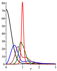
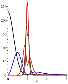
Figure 1: Energy density $T^{00}(r)$ for $r_{0}=1$ : a) (left) $\lambda=10$, $s=0.05$ (black), $s=0.09$ (blue), $s=0.15$ (brown), $s=0.25$ (dark green), $s=0.45$ (red); and b) (right) $\lambda=30$, $s=1/60$ (black), $s=0.03$ (blue), $s=0.1$ (brown), $s=0.2$ (dark green), $s=0.27$ (red).

The energy density of the $2$-dimensional defect is

$$T_{00} = \frac{\left(2\lambda s\right)^{2}}{r^{2}}\mathrm{sech}^{4}\left[2\lambda s\ln\left(\frac{r}{r_{0}}\right)\right]$$

$$~{}\times\left\{1+\left(\frac{1}{s}-2\right)\mathrm{sinh}^{2}\left[2\lambda s\ln\left(\frac{r}{r_{0}}\right)\right]\right\}$$

Here we consider $T_{00}$ finite in $r=0$, which restricts the parameters to satisfy $\lambda s\geq\frac{1}{2}$ when $\lambda>1$. The Figs. 1a-b depict the energy density $T_{00}\left(r\right)$ for fixed $r_{0}=1$ and several values of $\lambda$ and coupling constant $s$. We note that for fixed $\lambda>1$ and $\frac{1}{2\lambda}\leqslant s<\frac{1}{2}$, the behavior of the energy density changes from a lump centered in $r=0$ $\left(s=\frac{1}{2\lambda}\right)$ to a peak centered around $r_{0}$ $\left(s=\frac{1}{2}\right)$. For fixed $s$, the maximum amplitude of $T_{00}$ increases with $\lambda$, so large values of $\lambda$ produce more interesting results. For large values of $\lambda$, there exists a value $s_{0}$ so that for $\frac{1}{2\lambda}<s<s_{0}$, the effects of the field $\chi$ are strong and the defect appears as a thick tube structure whose center is localized between the origin and $r_{0}$. On the other hand, for $s_{0}\lesssim s<\frac{1}{2}$ it is clear the predominance of the field $\phi$ and the defect looks like as a thin tube centered around $r_{0}$.

This means that for larger values of $\lambda$ we can characterize the defect as a ring in the $2$-dimensional $yz$-plane, or as a cylindrical tube in the $3$-dimensional space, oriented along the symmetry $x$ axis. The influence of larger values of $s$ shows that the $\chi$ field is responsible for the process of generating a thicker tube. The total energy in the $yz$-plane is given by $E=8\pi\lambda/3$, which can be identified with the mass of the ring, $M_{ring}$.

III fermion localization

We are interested in the localization of (1,1)-dimensional fermions in an infinite tube whose transversal section is the 2-dimensional ring. Here, the tube in consideration is the one analyzed in the previous section. In considering fermionic states on a tube-like defect, we must remark that the analysis about the existence or not of fermionic zero modes was also considered in the other contexts. One can cite fermions in the field of an abelian and nonabelian string1 ; string2 ; string3 vortex solutions and more specifically neutrino zero modes on electroweak strings Zstring1 ; Zstring2 ; Zstring3 .

In the following we consider the fermionic field coordinates as $(x^{0},x^{1})=(t,x)$ and the ring coordinates as $(x^{2},x^{3})=(y,z)$. Then, after neglecting the backreaction on the tube, we consider the following fermionic action

$$S_{ferm}=\int\!\!dtdxdydz\!\!\left[\frac{{}}{{}}\bar{\Psi}\Gamma^{M}\partial_{M}\Psi-\eta F(\phi,\chi)\bar{\Psi}\Psi\right]\!,$$ (11)

where the $\Gamma^{0},\Gamma^{1}\$matrices are defined as

$$\Gamma^{0}=i\gamma^{0}=i\sigma^{1},~{}\Gamma^{1}=i\gamma^{1}=\sigma^{2},~{}$$ (12)

and $\Gamma^{2},\Gamma^{3}$ are conveniently chosen to provide Schrödinger’s equations in the $yz-$plane whose potentials are supersymmetric partners. Here $F(\phi(r),\chi(r))=F(r)$ is a function of the scalar fields $\phi(r)$ and $\chi(r)$ giving the ring solution in Eqs. (LABEL:solring) and $\eta$ is the coupling constant.

After transforming the $yz-$plane to polar coordinates, the equation of motion for $\Psi$ is found as

$$i\gamma^{\mu}\partial_{\mu}\Psi+\left(\begin{array}[]{cc}\partial_{r}+\frac{i}{r}\partial_{\theta}&0\\ 0&-(\partial_{r}-\frac{i}{r}\partial_{\theta})\end{array}\right)\Psi-\eta F\Psi=0$$ (13)

where Greek letters $\mu,\nu...$ are for the $(t,x)$ coordinates and we have chosen

$$\Gamma^{r}=\sigma^{3}=\left(\begin{array}[]{cc}1&0\\ 0&-1\end{array}\right)~{}\ ,~{}\ \ \Gamma^{\theta}=i\mathbf{1=}\left(\begin{array}[]{cc}i&0\\ 0&i\end{array}\right)\,.$$ (14)

We decouple the coordinates $(t,x)$ from $(r,\theta)$ by making the decomposition

$$\Psi\left(t,x,y,z\right)=\sum_{n}\left(\begin{array}[]{c}R_{n}\left(r,\theta\right)\Psi_{Rn}\left(t,x\right)\\ L_{n}\left(r,\theta\right)\Psi_{Ln}\left(t,x\right)\end{array}\right),$$ (15)

and by imposing that $\Psi_{Rn}$ and $\Psi_{Ln}$ are the chiral components of a fermion satisfying the (1+1)-dimensional Dirac’s equation

$$\left(i\gamma^{\mu}\partial_{\mu}-m\right)\left[\begin{array}[]{c}\Psi_{Rn}\\ \Psi_{Ln}\end{array}\right]=0\,,$$ (16)

we can rewrite Eq. (13) in the following set of equations for the chiral amplitudes $L_{n}(r,\theta)$ and $R_{n}(r,\theta)$:

$$\left(\partial_{r}-\frac{i}{r}\partial_{\theta}\right)L_{n}+\eta FL_{n} = m_{n}R_{n}\,,$$ (17)

$$-\left(\partial_{r}+\frac{i}{r}\partial_{\theta}\right)R_{n}+\eta FR_{n} = m_{n}L_{n}\,$$ (18)

Now we make the useful decomposition

$$L_{n}(r,\theta) = \sum_{\ell}\Lambda_{n\ell}(r)\,e^{i\ell\theta}$$ (19)

$$R_{n}(r,\theta) = \sum_{\ell}\varrho_{n\ell}(r)\,e^{i\ell\theta}$$ (20)

where $\ell\in Z$ and the functions $\Lambda_{n\ell}~{},~{}\varrho_{n\ell}$ are finite in $r=0$. Other decompositions are used in other contexts, see for instance, Refs. oda ; gog ; mello

By combining the Eqs. (17) and (18) we attain the Schrödinger-like equations for the scalar modes $\Lambda_{n\ell}(r)$ and $\varrho_{n}(r)$

$$-\frac{d^{2}\Lambda_{n\ell}}{dr^{2}}+V_{sch}^{L}(r)\Lambda_{n\ell} = \hat{H}_{sch}^{L}\Lambda_{n\ell}=m_{n}^{2}\Lambda_{n\ell}\,,$$ (21)

$$-\frac{d^{2}\varrho_{n\ell}}{dr^{2}}+V_{sch}^{R}(r)\varrho_{n\ell} = \hat{H}_{sch}^{R}\varrho_{n\ell}=m_{n}^{2}\varrho_{n\ell}$$ (22)

where the potentials are given by

$$V_{sch}^{L}(r) = \frac{\ell\left(\ell+1\right)}{r^{2}}+2\eta\ell\frac{F}{r}-\eta\left(\partial_{r}F\right)+\eta^{2}F^{2}\,,$$ (23)

$$V_{sch}^{R}(r) = \frac{\ell\left(\ell-1\right)}{r^{2}}+2\eta\ell\frac{F}{r}+\eta(\partial_{r}F)+\eta^{2}F^{2}\,.$$ (24)

Then, we have transformed the equation for fermions in a set of independent Schrödinger-like equations for the amplitudes $\Lambda_{n\ell}$ and $\varrho_{n\ell}$, allowing to get our goal of finding massive modes and analyzing their localization properties. The equations (21) and (22) allow us to adopt a probabilistic interpretation for finding massive modes of both chiralities in the tube. Here we are mainly interested in resonant states.

The Hamiltonians defining the Schrödinger-like equations, (21) and (22), can be rewritten in terms of the conjugate operators $\hat{A}$ and $\hat{A}^{{}^{{\dagger}}}$

$$\hat{A}=\frac{d}{dr}+\frac{\ell}{r}+\eta F~{}\ ,~{}\ \hat{A}^{{}^{{\dagger}}}=-\frac{d}{dr}+\frac{\ell}{r}+\eta F$$ (25)

as being $\ \hat{H}_{sch}^{L}=\hat{A}^{{}^{{\dagger}}}\hat{A}$ and $\hat{H}_{sch}^{R}=\hat{A}\hat{A}^{{}^{{\dagger}}}$, guaranteeing the eigenvalues $m_{n}^{2}$ to be nonnegative. In this way it is forbidden the existence of tachyonic modes. The eigenfunctions $\Lambda_{n\ell}$ and $\varrho_{n\ell}$ establish a complete set of orthonormal functions satisfying

$$\!\!\int\!\!dr\,\Lambda_{m\ell}\Lambda_{n\ell^{\prime}}=\delta_{mn}\delta_{\ell\ell^{\prime}}=\!\!\int\!\!dr\,\varrho_{m\ell}\varrho_{n\ell^{\prime}}~{},~{}\,\!\!\int\!\!dr\,\Lambda_{m\ell}\varrho_{n\ell^{\prime}}=0\,.$$ (26)

Further note that the action $S_{ferm}$ given by Eq. (11) can be integrated in the $(y,z)$ dimensions in order to obtain a standard action for massive Dirac fermions

$$S_{ferm}=\sum_{n}\int dt\,dx\,{\bar{\Psi}_{n}[\gamma^{\mu}\partial_{\mu}-m_{n}]\Psi_{n}}$$ (27)

Now we consider the issue of existence of the zero-mode $\chi_{0}$ which is obtained from

$$\hat{A}\chi_{0}=0$$ (28)

For fixed $\ell$ the hamiltonian $H_{sch}^{R}$ is a quantum mechanical supersymmetric partner of the hamiltonian $H_{sch}^{L}$  with superpotential

$$\mathcal{W}=\frac{\ell}{r}+\eta F,$$ (29)

hence the solution for the zero mode is

$$\chi_{0}\propto r^{-\ell}\exp\left\{-{\eta}\int_{0}^{r}dr^{\prime}F\left(r^{\prime}\right)\right\}.$$ (30)

In our analysis we are considering the Yukawa coupling, $F(\phi,\chi)=\phi(r)\chi(r)$. Hence, because the integral $\displaystyle{\int_{0}^{r}\!\!\!dr^{\prime}F(r^{\prime})}$ is finite for all $r$ the zero mode in non-normalizable for all $\ell$. Since the zero-mode of $H_{sch}^{L}$ is non-normalizable, we conclude that the spectra of $H_{sch}^{L}$ and $H_{sch}^{R}$ are identical due to the spontaneous breaking of supersymmetry in this quantum-mechanical system gan ; ortiz

IV Numerical Results

For our purposes we consider a simple Yukawa’s coupling, $F(\phi)=\phi\chi$. Interesting considerations for this and other couplings in models of two scalar fields can be found in cdh .

In order to investigate numerically the massive states, firstly we consider the region near the origin ( $r\ll r_{0}$) where

$$F\left(r\right)\sim-2\sqrt{\frac{1}{s}-2}\biggl{(}\frac{r}{r_{0}}\biggr{)}^{2\lambda s}.$$ (31)

Then for $\lambda s\geq 1/2$, the functions $F/r$, $\partial_{r}F$ and $F^{2}$ are finite and the potentials $V_{sch}^{L}(r)$ and$V_{sch}^{L}(r)$ are dominated by the contributions of the angular momentum proportional to $1/r^{2}$. In this way, for left chirality the potential is reduced to

$$\tilde{V}_{sch}^{L}(r)\approx\frac{\ell\left(\ell+1\right)}{r^{2}},$$ (32)

and the solutions finite in $r=0$ are

$$\Lambda_{n\ell}(r) = \sqrt{r}J_{\ell+\frac{1}{2}}(m_{n}r)~{},\ \ \ell\geq 1$$ (33)

$$\Lambda_{n\ell}\left(r\right) = \sqrt{r}Y_{\ell+\frac{1}{2}}\left(m_{n}r\right)\ ,\ \ell\leq-2,$$ (34)

$$\Lambda_{n\ell}(r) = \sqrt{r}Y_{\frac{1}{2}}(m_{n}r)~{},\ \ \ell=0,$$ (35)

$$\Lambda_{n\ell}(r) = \sqrt{r}J_{-\frac{1}{2}}(m_{n}r)~{},\ \ \ell=-1.$$ (36)

For right chirality we have

$$\tilde{V}_{sch}^{R}(r)\approx\frac{\ell^{2}-\ell}{r^{2}},$$ (37)

whose solutions finite in $r=0$ are

$$\varrho_{n\ell}(r) = \sqrt{r}Y_{\ell-\frac{1}{2}}(m_{n}r)~{},\ \ \ell\leq-1$$ (38)

$$\varrho_{n\ell}\left(r\right) = \sqrt{r}J_{\ell-\frac{1}{2}}\left(m_{n}r\right)\ ,\ \ell\geq 2,$$ (39)

$$\varrho_{n\ell}(r) = \sqrt{r}J_{-\frac{1}{2}}(m_{n}r)~{},\ \ \ell=0,$$ (40)

$$\varrho_{n\ell}(r) = \sqrt{r}Y_{\frac{1}{2}}(m_{n}r)~{},\ \ \ell=1.$$ (41)

Hence, for each value of $\ell$, Eqs. (33)-(36) or (38)-(41) are used as an input for the Runge-Kutta-Fehlberg method that produces a fifth order accurate solution.

We now define the probability for finding fermions inside the tube of radius $r_{0}$ as

$$P_{tube}={\frac{\displaystyle\int_{r_{min}}^{r_{0}}\!\!\!\!dr\,|\Psi_{n}(r)|^{2}}{\displaystyle\int_{r_{min}}^{r_{max}}\!\!\!\!dr\,|\Psi_{n}(r)|^{2}}}\,.$$ (42)

Here $r_{min}\ll r_{0}$ is used as the initial condition and $r_{max}$ is the characteristic box length used for the normalization procedure, being a value where the Schrödinger potentials are close to zero and where the massive modes oscillate as plane waves.

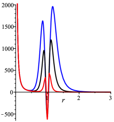
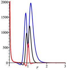
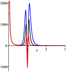
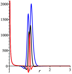
Figure 2: Schrödinger-like potentials $V_{sch}^{L}$ (left) and $V_{sch}^{R}$ (right) for $\ell=2$. We fix $r_{0}=1$, and $\eta=30$. We have a) $\lambda=30$ (upper figures) and b) $\lambda=50$ (lower figures). In all figures $s=0.1$(blue), $s=0.15$(black), $s=0.3$(red).

From the energy density considerations after Figs. 1a-1b, larger values of $\lambda$ favor the existence of a Schrödinger potential with structure similar a tube barrier em $r=r_{0}$.  The Fig. 2 depicts the Schrödinger-like potential $V_{sch}^{L}(r)$ and $V_{sch}^{R}(r)$ for $\ell=2$, $\lambda=30$, $50$, and fixed $\eta=30$ and $r_{0}=1$. The potentials in general diverge in $r\rightarrow 0$, assume a form of a barrier around $r=r_{0}$ and asymptote to zero as $r\rightarrow\infty$, indicating the possible presence of resonances. The increasing of $\eta$ turns the barrier of the potential higher, whereas the increasing of $\lambda$ turns it thinner. We noted that $\ell$ influences on the behavior of the potential for $r<r_{0}$ but has no sensible influence on the barrier and, we also observe that the increasing of $r_{0}$ turns the potential barrier wider.

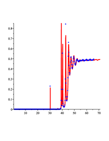
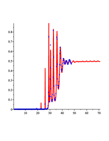
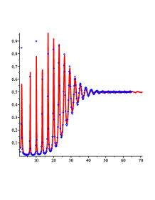
Figure 3: $P_{tube}(r)$ for left-(red line) and right-(dots) chirality fermions with $\ell=2$, $r_{0}=1$ $\eta=30$, $\lambda=30$, a) $s=0.10$, b) $s=0.15$, c) $s=0.30$.

Figs. 3a-c show some results of $P_{tube}(r)$  for left- and right-fermions. The plots are for $\ell=2$, $r_{0}=1$, $\eta=30$ and $\lambda=30$ and for various values of $s$. The plots shows several thin peaks of resonances. The thinner is the peak, the larger is the lifetime of the corresponding resonance. We note for $s\sim 0.10$ there are fewer but longer-lived resonance peaks, in comparison to $s\sim 0.30$. Note also that in general the masses of the resonances $m_{ress}$ increase gradually for lower values of $s$, but the relation $M_{ring}\ll m_{ress}$ was always verified, guaranteeing a condition for no backreaction of the fermions in the ring. The larger lifetime of the modes agrees with the correspondingly larger barrier of the Schrödinger-like potential around $r=r_{0}$ (compare with Figs. 2 ). This property of $V_{sch}$ is also responsible for the presence of resonance modes, in general, more massive for lower values of $s$ $\left(s\rightarrow\frac{1}{2\lambda}\right)$ which are closely related to the larger influence of the $\chi$ field in the internal structure of the defect. However, in this limit the number of the resonances is reduced because the mass values can not be higher than the tube-barrier. In this way, for finding long-lived resonances, there appears to be a physical compromise between a thinner tube (larger values of $s$ which unfavor the presence of the $\chi$ field) and the Yukawa coupling $\phi\chi$ (smaller values of $s$, related to a greater influence of the field $\chi$).

V Remarks and conclusions

We have studied the localization of (1+1)-dimensional fermionic fields in a generalized tube-like topological defect whose cross-section is a ring constructed with two scalar fields. Firstly, we have considered a general coupling between the defect and the fermion field carefully contructed to provide a supersymmetric quantum mechanical description of the chiral amplitudes related to the left- and right-fermionic components.  Consequently, the Hamiltonians describing the chiral amplitudes  are supersymmetric partners forbiding the existence of tachyonic modes. For the Yukawa coupling $F(\phi,\chi)=\eta\phi\chi$ it was shown that the zero-mode is non-normalizable and that the spectra of both chiralities are identical due to the spontaneous breaking of supersymmetry. Such result is corroborate by the numerical analysis of the Hamiltonian spectra.  Also, it was found that larger couplings $\eta$ and $\lambda$ are more effective for finding resonances after a fine-tuning of the contant $s$ characterizing the internal structure of the defect.

As a further comment we would like to point out that the Yukawa coupling is useful for studies of the electromagnetic charge of the ring and some effects like charge fractionalization. These studies are currently under consideration.

References

- (1) K. Akama, Lect. Notes Phys. 176, 267 (1982).
- (2) V. A. Rubakov and M. E. Shaposhnikov, Phys. Lett. B 125, 136 (1983).
- (3) V. A. Rubakov and M. E. Shaposhnikov, Phys. Lett. B 125, 139 (1983).
- (4) K. Akama, Gauge Theory and Gravitation, Proceedings, edited by K. Kikkawa, N. Nakanishi, and H. Nariai, Springer-Verlag, Nara, Japan (1983).
- (5) M. Visser, Phys. Lett. B 159, 22 (1985).
- (6) L. Randall and R. Sundrum, Phys. Rev. Lett. 83, 3370 (1999).
- (7) O. DeWolfe, D. Z. Freedman, S. S. Gubser and A. Karch, Phys. Rev. D 62, 046008 (2000).
- (8) M. Gremm, Phys. Lett. B 478, 434 (2000).
- (9) M. Gremm, Phys. Rev. D 62, 044017 (2000).
- (10) A. Kehagias and K. Tamvakis, Mod. Phys. Lett. A 17, 1767 (2002).
- (11) C. Csaki, J. Erlich, T. Hollowood and Y. Shirman, Nucl. Phys. B 581, 309 (2000).
- (12) A. Campos, Phys. Rev. Lett. 88, 141602 (2002).
- (13) R. Guerrero, A. Melfo and N. Pantoja, Phys. Rev. D 65, 125010 (2002).
- (14) D. Bazeia, C. Furtado and A. R. Gomes, J. Cosmol. Astropart. Phys. 0402 (2004) 002.
- (15) D. Bazeia and A. R. Gomes, J. High Energy Phys. 05 (2004) 012.
- (16) D. Bazeia, F. A. Brito and A. R. Gomes, J. High Energy Phys. 0411 (2004) 070.
- (17) V. Dzhunushaliev, V. Folomeev and M. Mina- mitsuji, Rep. Prog. Phys. 73, 066901 (2010).
- (18) R. Jackiw and C. Rebbi, Phys. Rev. D 13, 3398 (1976).
- (19) C. Ringeval, P. Peter, and J.-P. Uzan, Phys. Rev. D 65, 044016 (2002).
- (20) R. Davies and D. P. George, Phys. Rev. D 76, 104010 (2007).
- (21) Y.-X. Liu, Chun-E Fu, L. Zhao, and Y.-S. Duan, Phys. Rev. D 80, 065020 (2009).
- (22) S. L. Dubovsky, V. A. Rubakov, and P. G. Tinyakov, Phys. Rev. D 62, 105011 (2000).
- (23) C. A. S. Almeida, R. Casana, M. M. Ferreira, Jr., and A. R. Gomes, Phys. Rev. D 79, 125022 (2009).
- (24) Y.-X. Liu, J. Yang, Z.-H. Zhao, Chun-E Fu, and Y.-S. Duan, Phys. Rev. D 80, 065019 (2009).
- (25) Y.-X. Liu, H.-T. Li, Z.-H. Zhao, J.-X. Li, and J.-R. Ren, J. High Energy Phys. 10, 091 (2009).
- (26) Y.-X. Liu, Chun-E Fu, H. Guo, S.-W. Wei, and Z.-H. Zhao, JCAP 1012 (2010) 031.
- (27) W.T. Cruz, A.R. Gomes, C.A.S. Almeida, Eur.Phys.J. C71, 1790 (2011).
- (28) Chun-E Fu, Yu-Xiao Liu, Heng Guo, Phys. Rev. D 84, 044036 (2011).
- (29) Yu-Xiao Liu, Heng Guo, Chun-E Fu and Ji-Rong Ren, JHEP 02 (2010) 080.
- (30) D. Bazeia, J. Menezes, and R. Menezes, Phys. Rev. Lett. 91, 241601 (2003).
- (31) D. Bazeia, J. Menezes, R. Menezes, Mod. Phys. Lett. B19, 801 (2005).
- (32) R. Hobart, Proc. Phys. Soc. Lond.82, 201(1963).
- (33) G. H. Derrick J. Math. Phys. 5, 1252 (1964).
- (34) R. Rajaraman, “Solitons and Instantons”, North-Holland, Amsterdan, 1982.
- (35) M. Alford, J.A. Bowers, and K. Rajagopal, Phys. Rev. D 63, 074016 (2001).
- (36) M. G. Alford, K. Rajagopal, T. Schaefer, A. Schmitt, Rev.Mod.Phys.80, 1455 (2008).
- (37) R.Casalbuoni, R. Gatto, M. Mannarelli and G. Nardulli, Phys. Lett. B 511, 218 (2001);
- (38) R.Casalbuoni, R. Gatto, M. Mannarelli and G. Nardulli, Phys.Rev. D66 (2002) 014006.
- (39) F. Sannino, N. Marchal, W. Schäfer, Phys.Rev. D66 (2002) 016007.
- (40) N. Arkani-Hamed, S. Dimopoulos, G. Dvali, and N. Kaloper, Phys. Rev. Lett. 84, 586 (2000);
- (41) N. Kaloper, Phys. Lett. B 474, 269 (2000).
- (42) P.-M. Ho and Y.-T. Yeh, Phys. Rev. Lett. 85, 5523 (2000).
- (43) O. Bertolami and L. Guisado, J. High Energy Phys. 12, 013 (2003).
- (44) R.L. Dobrushin, Theor. Prob. Appl.17, 582 (1972).
- (45) C. Borgs, Commun. Math. Phys.96, 251 (1984)
- (46) D. Bazeia, M.J. dos Santos and R.F. Ribeiro, Phys. Lett. A208, 84 (1995).
- (47) M.A. Shifman and M.B. Voloshin, Phys. Rev. D 57, 2590 (1998).
- (48) A. Alonso Izquierdo, M.A. Gonzalez Leon, J. Mateos Guilarte, Phys. Rev. D 65, 085012 (2002).
- (49) A. de Souza Dutra, A. C. Amaro de Faria Jr, and M. Hott, Phys. Rev. D 78, 043526 (2008).
- (50) C. Nohl, Phys. Rev. D12, 1840 (1975).
- (51) H. deVega, Phys. Rev. D18, 2932 (1978).
- (52) R. Jackiw and P. Rossi, Nucl. Phys. B190, 681 (1981).
- (53) G. D. Starkman, D. Stojkovic, T. Vachaspati, Phys.Rev.D63, 085011 (2001).
- (54) D. Stojkovic, Int. J. Mod. Phys. A16, 1034 (2001).
- (55) G. Starkman, D. Stojkovic, T. Vachaspati, Phys.Rev.D65, 065003 (2002).
- (56) I. Oda, Phys.Rev. D62 (2000) 126009.
- (57) M. Gogberashvili, D. Singleton, Phys.Rev. D69 (2004) 026004.
- (58) E. R. Bezerra de Mello, J. High Energy Phys. 06 (2004) 016.
- (59) A. Gangopadhyaya, J. V. Mallow, C. Rasinariu, Supersymmetric Quantum Mechanis, World Scient. Publ., Singapore, 2011.
- (60) N. Fern´andez-Garc´ıa, O. Rosas-Ortiz, Int. J. Theor. Phys. 50, 2057 (2011).
- (61) R. A. C. Correa, A. de Souza Dutra, M. B. Hott, Class.Quant.Grav. 28, 155012 (2011).