Constraint on Heavy Element Production in Inhomogeneous Big-Bang Nucleosynthesis from The Light-Element Observations

Abstract

We investigate the observational constraints on the inhomogeneous big-bang nucleosynthesis that Matsuura et al [1] suggested the possibility of the heavy element production beyond ⁷Li in the early universe. From the observational constraints on light elements of ⁴He and D, possible regions are found on the plane of the volume fraction of the high density region against the ratio between high- and low-density regions. In these allowed regions, we have confirmed that the heavy elements beyond Ni can be produced appreciably, where $p$- and/or $r$-process elements are produced well simultaneously.

1 INTRODUCTION

Big-bang nucleosynthesis (BBN) has been investigated to explain the origin of the light elements, such as ⁴He, D, ³He, and ⁷Li, during the first few minutes [2, 3, 4]. Standard model of BBN (SBBN) can succeed to explain the observation of those elements,  ⁴He [5, 6, 34, 35], D [7, 8, 9, 36], and ³He [10, 11], except for ⁷Li. The study of SBBN has been done under the assumption of the homogeneous universe, where the model has only one parameter, the baryon-to-photon ratio $\eta$. If the present value of $\eta$ is determined, SBBN can be calculated from the thermodynamical history with use of the nuclear reaction network. We can obtain the reasonable value of $\eta$ by comparing the calculated abundances with observations. In the meanwhile, the value of $\eta$ is obtained as $\eta=\left(5.1-6.5\right)\times 10^{-10}$ [2] from the observations of ⁴He and D. This values agrees well with the observation of the cosmic microwave background: $\eta=\left(6.19\pm 0.14\right)\times 10^{-10}$ [12].

On the other hand, BBN with the inhomogeneous baryon distribution also has been investigated. The model is called as inhomogeneous BBN (IBBN). IBBN relies on the inhomogeneity of baryon concentrations that could be induced by baryogenesis (e.g. Ref. [13]) or phase transitions such as QCD or electro-weak phase transition [14, 15, 16] during the expansion of the universe. Although a large scale inhomogeneity is inhibited by many observations [12, 17], small scale one has been advocated within the present accuracy of the observations. Therefore, it remains a possibility for IBBN to occur in some degree during the early era. In IBBN, the heavy element nucleosynthesis beyond the mass number $A=8$ has been proposed [13, 14, 18, 19, 20, 21, 22, 23, 24]. In addition, peculiar observations of abundances for heavy elements and/or ⁴He could be understood in the way of IBBN. For example, the quasar metallicity of C, N, and Si could have been explained from IBBN [25]. Furthermore, from recent observations of globular clusters, possibility of inhomogeneous helium distribution is pointed out [26], where some separate groups of different main sequences in blue band of low mass stars are assumed due to high primordial helium abundances compared to the standard value [27, 28]. Although baryogenesis could be the origin of the inhomogeneity, the mechanism of it has not been clarified due to unknown properties of the supersymmetric Grand Unified Theory [29].

Despite a negative opinion against IBBN due to insufficient consideration of the scale of the inhomogeneity [30], Matsuura et al. have found that the heavy element synthesis for both $p$- and $r$-processes is possible if $\eta>10^{-4}$ [1], where they have also shown that the high $\eta$ regions are compatible with the observations of the light elements, ⁴He and D [31]. However, their analysis is only limited to a parameter of a specific baryon number concentration. In this paper, we extend the investigations of Matsuura et al. [1, 31] to check the validity of their conclusion from a wide parameter space of the IBBN model.

In §2, we review and give the adopted model of IBBN which is the same one as that of Matsuura et al. [31]. Constraints on the critical parameters of IBBN due to light element observations are shown in §III, and the possible heavy element nucleosynthesis are presented in §IV. Finally, §5 are devoted to the summary and discussion.

2 Model

In this section, we introduce the model of IBBN. We adopt the two-zone model for the inhomogeneous BBN. In IBBN model, we assume the existence of spherical high-density region inside the horizon. For simplicity, we ignore in the present study the diffusion effects before $\left(10^{10}{\rm K}<T<10^{11}{\rm K}\right)$ and during the primordial nucleosynthesis $\left(10^{7}{\rm K}<T<10^{10}{\rm K}\right)$, because the timescale of the neutron diffusion is longer than that of the cosmic expansion [18, 26].

To find the parameters compatible with the observations, we consider the averaged abundances between the high- and low-density regions. We get at least parameters for the extreme case by averaging the abundances in two regions. Let us define the notations, $n_{ave},n_{high}$, and $n_{low}$ as averaged-, high-, and low- baryon number densities. $f_{v}$ is the volume fraction of the high baryon density region. $X^{ave}_{i},X^{high}_{i}$ and $X^{low}_{i}$ are mass fractions of each element $i$ in averaged-, high- and low-density regions, respectively, Then, basic relations are written as follows [31]:

$$n_{ave} = f_{v}n_{high}+\left(1-f_{v}\right)n_{low},$$ (1)

$$n_{ave}X^{ave}_{i} = f_{v}n_{high}X^{high}_{i}+\left(1-f_{v}\right)n_{low}X^{low}_{i}.$$ (2)

Here we assume the baryon fluctuation to be isothermal as was done in previous studies (e.g., Refs. [14, 15, 20]). Under that assumption, since the baryon-to-photon ratio is defined by the number density of photon in standard BBN, Eqs. (1) and (2) are rewritten as follows:

$$\eta_{ave} = f_{v}\eta_{high}+(1-f_{v})\eta_{low},$$ (3)

$$\eta_{ave}X^{ave}_{i} = f_{v}X^{high}_{i}\eta_{high}+(1-f_{v})X^{low}_{i}\eta_{low},$$ (4)

where $\eta$s with subscripts are the baryon-to-photon ratios in each region. In the present paper, we fix $\eta_{ave}=6.19\times 10^{-10}$ from the cosmic microwave background observation [12]. The values of $\eta_{high}$ and $\eta_{low}$ are obtained from both $f_{v}$ and the density ratio between high- and low-density region: $R\equiv n_{high}/n_{low}=\eta_{high}/\eta_{low}$.

To calculate the evolution of the universe, we solve the following Friedmann equation,

$$\left(\frac{\dot{x}}{x}\right)^{2}=\frac{8\pi G}{3}\rho,$$ (5)

where $x$ is the cosmic scale factor and $G$ is the gravitational constant. The total energy density $\rho$ in Eq. (5) is the sum of decomposed parts:

$$\rho=\rho_{\gamma}+\rho_{\nu}+\rho_{e^{\pm}}+\rho_{b}.$$ (6)

Here the subscripts $\gamma,\nu$, and $e^{\pm}$ indicate photons, neutrino, and electrons/positrons, respectively. The final term is the baryon density obtained as $\rho_{b}\simeq m_{p}n_{ave}$.

We should note about the energy density of baryon. To get the time evolution of the baryon density in both regions, the energy conservation law is used:

$$\frac{d}{dt}(\rho x^{3})+p\frac{d}{dt}(x^{3})=0,$$ (7)

where $p$ is the pressure of the fluid. When we solve Eq. (7), initial values in both regions are obtained from Eq. (3) with $f_{v}$ and $R$ fixed. For $\eta_{high}\geq 2\times 10^{-4}$, the baryon density in the high-density region, $\rho_{high}$, is larger than the radiation component at $T>10^{9}$ K. However, we note that the contribute to eq. (6) is not $\rho_{high}$, but $f_{v}\rho_{high}$. In our research, the ratio of $f_{v}\rho_{high}$ to $\rho_{\gamma}$ is about $10^{-7}$ at BBN epoch. Therefore, we can neglect the final term of eq. (6) in the same way as has been done in SBBN during the calculation of eq.(5).

3 Constraints from light-element observations

In this section, we calculate the nucleosynthesis in high- and low-density regions with use of the BBN code [32] which includes 24 nuclei from neutron to ¹⁶O. We adopt the reaction rates of Descouvemont et al. [33], the neutron lifetime $\tau_{N}=885.7$ sec [2], and consider three massless neutrinos.

Let us consider the range of $f_{v}$. For $f_{v}\ll 0.1$, the heavier elements can be synthesized in the high-density regions as discussed in Ref. [22]. For $f_{v}>0.1$, contribution of the low-density region to $\eta_{ave}$ can be neglected and therefore to be consistent with observations of light elements, we need to impose the condition of $f_{v}<0.1$.

Figure 1 illustrates the light element synthesis in the high- and low-density regions with $f_{v}=10^{-6}$ and $R=10^{6}$ that corresponds to $\eta_{high}=3.05\times 10^{-4}$ and $\eta_{low}=3.05\times 10^{-10}$. Light elements synthesized in these calculations are shown in Table 1. In the low-density region the evolution of the elements is almost the same as the case of SBBN. In the high-density region, while ⁴He is more abundant than that in the low-density region, ⁷Li (or ⁷Be) is much less produced. In this case, we can see that average values such as ⁴He and D are overproduced as shown in Table 1. However, this overproduction can be saved by choosing the parameters carefully; We need to find the reasonable parameter ranges for both $f_{v}$ and $R$ by comparing with the observation of the light elements.

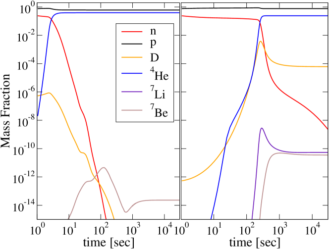
Fig. 1: Illustration of the nucleosynthesis in the two-zone IBBN model with $f_{v}=10^{-6}$ and $R=10^{6}$. The baryon-to-photon ratios in the high- (left panel) and low- (right panel) density regions are $\eta_{high}=3.05\times 10^{-4}$ and $\eta_{low}=3.05\times 10^{-10}$, respectively.

Table. 1: The numerical abundances of light elements synthesized as shown in Figure 1.

Elements	$X^{high}_{i}$	$X^{low}_{i}$	$X_{i}$
p	$0.608$	$0.759$	$0.684$
D	$3.07\times 10^{-18}$	$1.19\times 10^{-4}$	$5.95\times 10^{-5}$
T +3He	$1.15\times 10^{-13}$	$3.41\times 10^{-5}$	$1.71\times 10^{-5}$
4He	$0.392$	$0.241$	$0.316$
7Li + 7Be	$8.2\times 10^{-13}$	$6.29\times 10^{-10}$	$3.14\times 10^{-10}$

Now, we put constraints on $f_{v}$ and $R$ by comparing the average values of ⁴He and D obtained from Eq. (4) with the following observational values. First we consider the primordial ⁴He abundance reported in Ref.[34]:

$$Y_{p}=0.2565\pm 0.0010\pm 0.0050,$$

and Ref.[35]:

$$Y_{p}=0.2534\pm 0.0083.$$

We adopt ⁴He abundances as follows:

$$0.2415<Y_{p}<0.2617.$$ (8)

Next, we take the primordial abundance from the D/H observation reported in Ref. [9]:

$$\text{D/H}=\left(2.84\pm 0.26\right)\times 10^{-5},$$

and Ref. [36]:

D/H $$= \left(2.535\pm 0.05\right)\times 10^{-5},$$

D/H $$= \left(2.48\pm 0.12\right)\times 10^{-5}.$$

Considering those observations with errors, we adopt the primordial D/H abundance as follows:

$$2.36<\text{D/H}\times 10^{5}<3.02.$$ (9)

Figure 2 illustrates the constraints on the $f_{v}-R$ plane from the above light-element observations with contours of constant $\eta_{high}$. The solid and dashed lines indicate the upper limits from Eqs. (8) and (9), respectively. As the results, we can obtain approximately the following relations between $f_{v}$ and $R$ :

$$R\leq\begin{cases}10^{4}\times f_{v}^{-0.3}&\text{~{}for~{}}f_{v}>7.4\times 10^{-6},\\ 0.13\times f_{v}^{-0.98}&\text{~{}for~{}}f_{v}\leq 7.4\times 10^{-6}.\end{cases}$$ (10)

The ⁴He observation (8) gives the upper bound for $f_{v}<7.4\times 10^{-6}$, and the limit for $f_{v}>7.4\times 10^{-6}$ is obtained from D observation (9). As shown in Figure 2, we can find the allowed regions which include the very high-density region such as $\eta_{high}=10^{-3}$.

We should note that $\eta_{high}$ takes larger value, nuclei which are heavier than ⁷Li are synthesized more and more. Then we can estimate the amount of total CNO elements in the allowed region. Figure 3 illustrates the contours of the summation of the average values of the heavier nuclei ($A>7$), which correspond to Figure 2 and are drawn using the constraint from ⁴He and D/H observations . As a consequence, we get the upper limit of total mass fractions for heavier nuclei as follows:

$$X(A>7)\leq 10^{-5}.$$

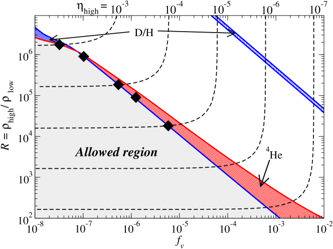
Fig. 2: Constraints on the $f_{v}-R$ plane from the observations of light element abundances. The region below the red line is allowable one obtained from ⁴He observation (8). Constraints from the D/H observation (9) are shown by the region below the blue line. The gray region corresponds to the allowable parameters determined from the two observations of ⁴He and D/H. There is another region which is still consistent with only D/H in the upper right direction. This is the contribution of the low density region with $\eta_{low}\sim 10^{-12}$; The D abundance tends to decrease against the baryon density for $\eta>10^{-12}$. The dotted lines show the contours of the baryon-to-photon ratio in the high-density region. Filled squares indicate the parameters for heavy element nucleosynthesis adopted in §4.

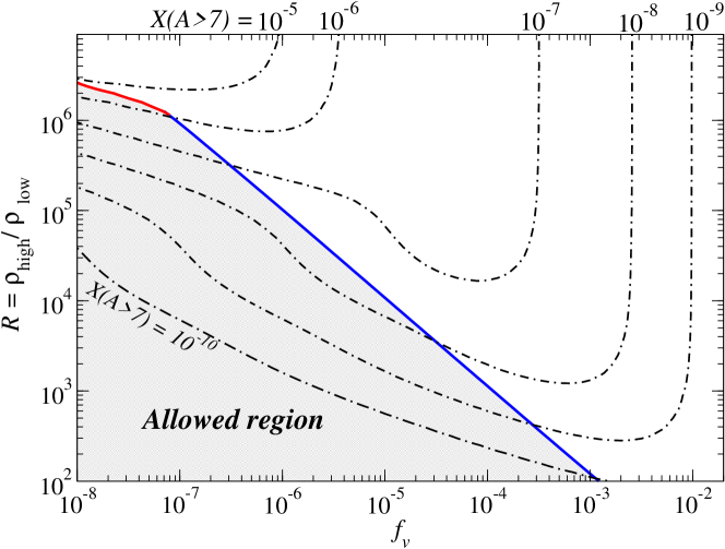
Fig. 3: Contours of the averaged total mass fractions which are the sum of nuclei heavier than ⁷Li, where we find consistent region of the produced elements with ⁴He and D observations.

4 Heavy element Production

In the previous section, we have obtained the amount of CNO elements produced in the two-zone IBBN model. However, it is not enough to examine the nuclear production beyond $A>8$ because the baryon density in the high-density region becomes so high that elements beyond CNO isotopes can be produced [1, 13, 21, 23]. In this section, we investigate the heavy element nucleosynthesis in the high-density region considering the constraints shown in Figure 2. Abundance change is calculated with a large nuclear reaction network, which includes 4463 nuclei from neutron $(n)$, proton $(p)$ to Americium (Z = 95 and A = 292). Nuclear data, such as reaction rates, nuclear masses, and partition functions, are the same as used in [37] except for the neutron-proton interaction; We use the weak interaction of Kawano code [38], which is adequate for the high temperature epoch of $T>10^{10}$ K.

As seen in Figure 3, heavy elements of $X(A>7)>10^{-9}$ are produced nearly along the upper limit of $R$. Therefore, to examine the efficiency of the heavy element production, we select five models with the following parameters: $\eta_{high}=10^{-3},5.1\times 10^{-4},10^{-4},5.0\times 10^{-5}$ , and $10^{-5}$ corresponded to $\left(f_{v},R\right)=\left(3.24\times 10^{-8},1.74\times 10^{6}\right)$ , $\left(1.03\times 10^{-8},9.00\times 10^{5}\right)$ , $\left(5.41\times 10^{-7},1.84\times 10^{5}\right)$ , $\left(1.50\times 10^{-6},9.20\times 10^{4}\right)$ , and $\left(5.87\times 10^{-6},1.82\times 10^{4}\right)$. Adopted parameters are indicated by filled squares in Figure 2.

First, we evaluate the validity of the nucleosynthesis code with $4463$ nuclei. Table 2 shows the results of the light elements, p, D, ⁴He, ³He, and ⁷Li. The results of the high-density region is calculated by the extended nucleosynthesis code, and the abundances in the low-density region is obtained by BBN code.The averaged abundances is obtained by Eq. (4). Since the averaged values of ⁴He and D are consistent with the observations, there is no difference between BBN code and the extended nucleosynthesis code in regard to the averaged abundances of light elements.

Table. 2: Mass fractions of light elements for the four cases : $\eta_{high}\simeq 10^{-3}$, $\eta_{high}=5\times 10^{-4}$, $\eta_{high}\simeq 10^{-4}$, and $\eta_{high}=10^{-5}$. $t_{fin}$ and $T_{fin}$ is the time and temperature at the final stage of the calculations.

$f_{v},R$	$3.23\times 10^{-8},1.74\times 10^{6}$			$1.03\times 10^{-7},9.00\times 10^{5}$
$(\eta_{high},\eta_{low})$	($1.02\times 10^{-3}$, $5.86\times 10^{-10}$)			($5.10\times 10^{-4}$, $5.67\times 10^{-10}$)
$\left(t_{fin},T_{fin}\right)$	$1.0\times 10^{5}$sec, $4.2\times 10^{7}$ K			$1.1\times 10^{5}$sec, $4.9\times 10^{7}$ K
elements	high	low	average	high	low	average
p	$0.586$	$0.753$	$0.744$	$0.600$	$0.753$	$0.740$
D	$1.76\times 10^{-21}$	$4.50\times 10^{-5}$	$4.26\times 10^{-5}$	$3.43\times 10^{-21}$	$4.75\times 10^{-5}$	$4.34\times 10^{-5}$
3He+T	$2.91\times 10^{-14}$	$2.18\times 10^{-5}$	$2.07\times 10^{-5}$	$2.77\times 10^{-14}$	$2.23\times 10^{-5}$	$2.04\times 10^{-5}$
4He	$0.413$	$0.247$	$0.256$	$0.400$	$0.247$	$0.260$
7Li+7Be	$1.63\times 10^{-13}$	$1.78\times 10^{-9}$	$1.68\times 10^{-9}$	$6.80\times 10^{-14}$	$1.65\times 10^{-9}$	$1.52\times 10^{-9}$

(a) For cases of $\eta_{high}=10^{-3}$ and $\eta_{high}=5\times 10^{-4}$.

$f_{v},R$	$5.41\times 10^{-7},1.84\times 10^{5}$			$5.87\times 10^{-6},1.82\times 10^{4}$
$(\eta_{high},\eta_{low})$	($1.04\times 10^{-4}$, $5.62\times 10^{-10}$)			($1.02\times 10^{-5}$, $5.59\times 10^{-10}$)
$\left(t_{fin},T_{fin}\right)$	$1.2\times 10^{5}$sec, $4.3\times 10^{7}$ K			$1.2\times 10^{5}$sec, $4.5\times 10^{7}$ K
elements	high	low	average	high	low	average
p	$0.638$	$0.753$	$0.742$	$0.670$	$0.753$	$0.745$
D	$6.84\times 10^{-22}$	$4.79\times 10^{-5}$	$4.36\times 10^{-5}$	$1.12\times 10^{-22}$	$4.48\times 10^{-5}$	$4.37\times 10^{-5}$
3He+T	$1.63\times 10^{-13}$	$2.23\times 10^{-5}$	$2.04\times 10^{-5}$	$1.49\times 10^{-9}$	$2.25\times 10^{-5}$	$2.03\times 10^{-5}$
4He	$0.362$	$0.247$	$0.258$	$0.330$	$0.247$	$0.254$
7Li+7Be	$7.42\times 10^{-13}$	$1.64\times 10^{-9}$	$1.49\times 10^{-9}$	$6.73\times 10^{-8}$	$1.62\times 10^{-9}$	$7.96\times 10^{-9}$

(b) For cases of $\eta_{high}=10^{-4}$ and $\eta_{high}=10^{-5}$.

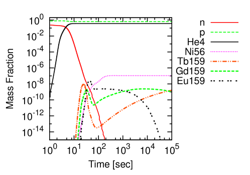
(a) $\eta_{high}=1.02\times 10^{-4}$

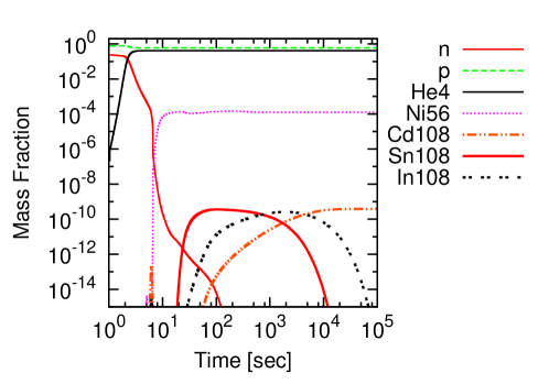
(b) $\eta_{high}=1.06\times 10^{-3}$

Fig. 4: Time evolution of the mass fractions in high-density regions of (a) $\eta_{high}=1.02\times 10^{-4}$ and (b) $\eta_{high}=1.06\times 10^{-3}$.

Figure 4 shows the results of nucleosynthesis in the high-density regions with $\eta_{high}\simeq 10^{-4}$ and $10^{-3}$. In Figure 4(a), we see the time evolution of the abundances of Gd and Eu for the mass number 159. First ¹⁵⁹Tb (stable $r$-element) is synthesized and later ¹⁵⁹Gd and ¹⁵⁹Eu are synthesized through the neutron captures. After $t=10^{3}$ sec, ¹⁵⁹Eu decays to nuclei by way of ¹⁵⁹Eu $\rightarrow{}^{159}$Gd$\rightarrow{}^{159}$Tb, where the half-life of ¹⁵⁹Eu and ¹⁵⁹Gd are $26.1$ min and $18.479$ h, respectively.

For $\eta_{high}\simeq 10^{-3}$, the result is seen in Figure 4(b). ¹⁰⁸Sn which is proton-rich nuclei is synthesized. After that, stable nuclei ¹⁰⁸Cd is synthesized by way of ¹⁰⁸Sn $\rightarrow{}^{108}$In $\rightarrow{}^{108}$Cd, where the half-life of ¹⁰⁸Sn and ¹⁰⁸In are $10.3$ min and $58.0$ min, respectively. These results are qualitatively the same as Matsuura et al. [1].

In addition, we notice the production of radioactive nuclei of ⁵⁶Ni and ⁵⁷Co, where ⁵⁶Ni is produced at early times, just after the formation of ⁴He. Usually, nuclei such as ⁵⁶Ni and ⁵⁷Co are produced in supernova explosions, which are assumed to be the events after the first star formation (e.g. Ref. [40]). In IBBN model, however, this production can be found to occur at extremely high density region of $\eta_{high}\geq 10^{-3}$ as the primary elements without supernova events in the early universe.

Final results ($T=4\times 10^{7}$ K) of nucleosynthesis calculations are shown in Table. 3. When we calculate the average values, we set the abundances of $A>16$ to be zero for low-density side. For $\eta_{high}\simeq 10^{-4}$, a lot of nuclei of $A>7$ are synthesized whose amounts are comparable to that of ⁷Li. Produced elements in this case include both $s$-element (i.e., ¹³⁸Ba) and $r$-elements (for instance, ¹⁴²Ce and ¹⁴⁸Nd). For $\eta_{high}\simeq 10^{-3}$, there are few $r$-elements while both $s$-elements (i.e., ⁸²Kr and ⁸⁹Y) and $p$-elements (i.e., ⁷⁴Se and ⁷⁸Kr) are synthesized such as the case of supernova explosions. For $\eta_{high}=10^{-3}$ the heavy elements are produced slightly more than the total mass fraction (shown in Figure 3) derived from the BBN code calculations. This is because our BBN code used in §3 includes the elements up to $A=16$ and the actual abundance flow proceeds to much heavier elements.

Figure 5 shows the abundances averaged between high- and low-density region using eq. (4) comparing with the solar system abundances [39]. For $\eta_{high}\simeq 10^{-4}$, abundance productions of $120<A<180$ are comparable to the solar values. For $\eta_{high}\simeq 10^{-3}$, those of $50<A<100$ have been synthesized well. In the case of $\eta_{high}=5\times 10^{-4}$, there are outstanding two peaks; one is around $A=56~{}(N=28)$ and the other can be found around $A=140$. Abundance patterns are very different from that of the solar system ones, because IBBN occurs under the condition of significant amount of abundances of both neutrons and protons.

Table. 3: Mass fractions of heavy elements $(A~{}>~{}7)$ for three cases of $\eta_{high}\simeq 10^{-3},\eta_{high}=5.33\times 10^{-4}$, and $\eta_{high}\simeq 10^{-4}$.

$f_{v}=3.23\times 10^{-8},R=1.74\times 10^{6}$			$f_{v}=1.03\times 10^{-7},R=9.00\times 10^{5}$			$f_{v}=5.41\times 10^{-7},R=1.84\times 10^{5}$
$\left(\eta_{high}=1.06\times 10^{-3}\right)$			$\left(\eta_{high}=5.33\times 10^{-4}\right)$			$\left(\eta_{high}=1.02\times 10^{-4}\right)$
element	high	average	element	high	average	element	high	average
Ni56	$1.247\times 10^{-4}$	$6.658\times 10^{-6}$	Nd142	$2.051\times 10^{-5}$	$1.738\times 10^{-6}$	Nd145	$3.692\times 10^{-7}$	$3.342\times 10^{-8}$
Co57	$1.590\times 10^{-5}$	$8.487\times 10^{-7}$	Ni56	$1.270\times 10^{-5}$	$1.077\times 10^{-6}$	Ca40	$2.706\times 10^{-7}$	$2.450\times 10^{-8}$
Sr86	$1.061\times 10^{-5}$	$5.662\times 10^{-7}$	Sm148	$1.059\times 10^{-5}$	$8.976\times 10^{-7}$	Mn52	$2.417\times 10^{-7}$	$2.188\times 10^{-8}$
Sr87	$9.772\times 10^{-6}$	$5.214\times 10^{-7}$	Pm147	$6.996\times 10^{-6}$	$5.930\times 10^{-7}$	Eu155	$2.374\times 10^{-7}$	$2.149\times 10^{-8}$
Se74	$9.745\times 10^{-6}$	$5.200\times 10^{-7}$	Pm145	$6.559\times 10^{-6}$	$5.559\times 10^{-7}$	Ce140	$1.931\times 10^{-7}$	$1.748\times 10^{-8}$
Sr84	$9.172\times 10^{-6}$	$4.894\times 10^{-7}$	Sm146	$6.539\times 10^{-6}$	$5.542\times 10^{-7}$	Cr51	$1.546\times 10^{-7}$	$1.400\times 10^{-8}$
Kr82	$8.910\times 10^{-6}$	$4.754\times 10^{-7}$	Nd143	$4.146\times 10^{-6}$	$3.514\times 10^{-7}$	Ce142	$1.114\times 10^{-7}$	$1.008\times 10^{-8}$
Kr81	$7.797\times 10^{-6}$	$4.160\times 10^{-7}$	Pr141	$3.957\times 10^{-6}$	$3.354\times 10^{-7}$	Ni56	$1.100\times 10^{-7}$	$9.964\times 10^{-9}$
Ge72	$7.674\times 10^{-6}$	$4.095\times 10^{-7}$	Nd144	$3.952\times 10^{-6}$	$3.350\times 10^{-7}$	Nd146	$1.049\times 10^{-7}$	$9.501\times 10^{-9}$
Kr78	$7.602\times 10^{-6}$	$4.057\times 10^{-7}$	Sm147	$3.752\times 10^{-6}$	$3.180\times 10^{-7}$	Eu156	$9.436\times 10^{-8}$	$8.542\times 10^{-9}$
Kr80	$7.063\times 10^{-6}$	$3.769\times 10^{-7}$	Sm149	$3.322\times 10^{-6}$	$2.815\times 10^{-7}$	Nd148	$9.361\times 10^{-8}$	$8.474\times 10^{-9}$
Kr83	$6.252\times 10^{-6}$	$3.336\times 10^{-7}$	Pm146	$2.629\times 10^{-6}$	$2.228\times 10^{-7}$	Fe52	$8.974\times 10^{-8}$	$8.124\times 10^{-9}$
Ge73	$6.144\times 10^{-6}$	$3.278\times 10^{-7}$	Sm144	$2.207\times 10^{-6}$	$1.870\times 10^{-7}$	Tb161	$8.956\times 10^{-8}$	$8.108\times 10^{-9}$
Se76	$5.929\times 10^{-6}$	$3.164\times 10^{-7}$	Sm150	$1.683\times 10^{-6}$	$1.426\times 10^{-7}$	La139	$8.804\times 10^{-8}$	$7.971\times 10^{-9}$
Br79	$5.904\times 10^{-6}$	$3.150\times 10^{-7}$	Pm144	$1.581\times 10^{-6}$	$1.340\times 10^{-7}$	N14	$8.736\times 10^{-8}$	$7.909\times 10^{-9}$
Se77	$5.345\times 10^{-6}$	$2.852\times 10^{-7}$	Pm143	$1.575\times 10^{-6}$	$1.335\times 10^{-7}$	Cr48	$8.561\times 10^{-8}$	$7.750\times 10^{-9}$
Y89	$4.759\times 10^{-6}$	$2.539\times 10^{-7}$	Sm145	$1.010\times 10^{-6}$	$8.568\times 10^{-8}$	Ba138	$7.955\times 10^{-8}$	$7.202\times 10^{-9}$
Zr90	$4.412\times 10^{-6}$	$2.354\times 10^{-7}$	Co57	$8.643\times 10^{-7}$	$7.326\times 10^{-8}$	C12	$7.672\times 10^{-8}$	$6.945\times 10^{-9}$
Rb85	$4.324\times 10^{-6}$	$2.307\times 10^{-7}$	Eu153	$5.563\times 10^{-7}$	$4.715\times 10^{-8}$	Dy162	$6.835\times 10^{-8}$	$6.188\times 10^{-9}$
Rb83	$4.082\times 10^{-6}$	$2.178\times 10^{-7}$	Ce140	$4.944\times 10^{-7}$	$4.191\times 10^{-8}$	C13	$6.428\times 10^{-8}$	$5.819\times 10^{-9}$
Y88	$3.845\times 10^{-6}$	$2.052\times 10^{-7}$	Nd145	$4.376\times 10^{-7}$	$3.709\times 10^{-8}$	O16	$6.301\times 10^{-8}$	$5.704\times 10^{-9}$
Zr88	$3.546\times 10^{-6}$	$1.892\times 10^{-7}$	Eu155	$4.224\times 10^{-7}$	$3.581\times 10^{-8}$	Gd158	$5.845\times 10^{-8}$	$5.292\times 10^{-9}$
As73	$3.519\times 10^{-6}$	$1.878\times 10^{-7}$	Eu151	$4.106\times 10^{-7}$	$3.480\times 10^{-8}$	Cs137	$5.559\times 10^{-8}$	$5.033\times 10^{-9}$
Ga71	$3.388\times 10^{-6}$	$1.808\times 10^{-7}$	Cr52	$4.071\times 10^{-7}$	$3.450\times 10^{-8}$	Nd147	$3.962\times 10^{-8}$	$3.587\times 10^{-9}$
Se75	$2.933\times 10^{-6}$	$1.565\times 10^{-7}$	Cd108	$3.596\times 10^{-7}$	$3.048\times 10^{-8}$	Ho165	$3.770\times 10^{-8}$	$3.413\times 10^{-9}$
Nb91	$2.896\times 10^{-6}$	$1.545\times 10^{-7}$	Gd156	$3.368\times 10^{-7}$	$2.854\times 10^{-8}$	Pr143	$3.111\times 10^{-8}$	$2.817\times 10^{-9}$
As75	$2.856\times 10^{-6}$	$1.524\times 10^{-7}$	Cd110	$3.103\times 10^{-7}$	$2.630\times 10^{-8}$	Ce141	$2.998\times 10^{-8}$	$2.714\times 10^{-9}$
Mo92	$2.442\times 10^{-6}$	$1.303\times 10^{-7}$	Eu152	$2.809\times 10^{-7}$	$2.381\times 10^{-8}$	Gd160	$2.950\times 10^{-8}$	$2.670\times 10^{-9}$
Ge70	$2.318\times 10^{-6}$	$1.237\times 10^{-7}$	Sm151	$2.795\times 10^{-7}$	$2.369\times 10^{-8}$	Xe136	$2.771\times 10^{-8}$	$2.509\times 10^{-9}$
Sr88	$2.021\times 10^{-6}$	$1.078\times 10^{-7}$	Eu154	$2.759\times 10^{-7}$	$2.339\times 10^{-8}$	Xe134	$2.238\times 10^{-8}$	$2.026\times 10^{-9}$
$\displaystyle\sum_{A>7}{X(A)}$	$3.010\times 10^{-4}$	$1.652\times 10^{-5}$	$\displaystyle\sum_{A>7}{X(A)}$	$1.062\times 10^{-4}$	$9.006\times 10^{-6}$	$\displaystyle\sum_{A>7}{X(A)}$	$3.850\times 10^{-6}$	$3.485\times 10^{-7}$

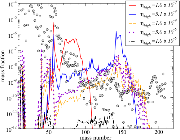
Fig. 5: Comparison of the averaged mass fractions in the two-zone model with the solar system abundances [39] (indicated by dots).

5 Summary and Discussion

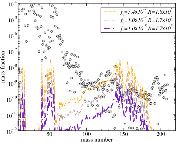
Fig. 6: Same as Fig. 5, but $\eta_{high}$ is fixed as $10^{-4}$.

We extend previous studies of Matsuura et al. [1, 31] and investigate the consistency between the light-element abundances in the IBBN model and the observation of ⁴He and D/H.

First, we have done the nucleosynthesis calculation using the BBN code with 24 nuclei for the both regions. The time evolution of the light-elements at the high-density region differs significantly from that at the low-density region; The nucleosynthesis begins faster and ⁴He is more abundant than that in the low density region. By comparing the average abundances with ⁴He and D/H observations, we can get the allowable parameters of the two-zone model: the volume fraction $f_{v}$ of the high-density region and the density ratio $R$ between the two regions.

Second, we calculate the nucleosynthesis that includes 4463 nuclei in the high-density regions. Qualitatively, results of nucleosynthesis are the same as those in Ref. [1]. In the present results, we showed that $p$- and $r$-elements are synthesized simultaneously at high-density region with $\eta_{high}\simeq 10^{-4}$.

We find that the average mass fractions in IBBN amount to as much as the solar system abundances. As see from Figure 5, there are over-produced elements around $A=150$ (for $\eta_{high}=10^{-4}$) and $A=80$ (for $\eta_{high}=10^{-3}$). Although it seems to conflict with the chemical evolution in the universe, this problem could be solved by the careful choice of $f_{v}$ and/or $R$. Figure 6 illustrates the mass fractions with $\eta_{high}=1.0\times 10^{-4}$ for three sets of $f_{v}-R$. It is shown that the abundances can become lower than the solar system abundances. If we put constraint on the $f_{v}-R$ plane from the heavy element observations [45, 46, 47, 48], the parameters in IBBN model should be tightly determined.

In the meanwhile, we would like to touch on the consistency against the primordial ⁷Li. We have obtained interesting results about ⁷Li abundances in our model. For the recent study of ⁷Li, the lithium problem arises from the discrepancy among ⁷Li abundance predicted by SBBN theory, the baryon density of WMAP, and abundance inferred from observations of metal-poor stars (see Refs. [42, 43]). As seen in Table 2, ⁷Li is clearly overproduced such as ⁷Li/H$|_{ave}=1.52\times 10^{-9}$ for $\eta_{high}=10^{-5}$, although we adopt the highest observational value ⁷Li/H$=\left(2.75-4.17\right)\times 10^{-10}$ [44]. However, for cases of $\eta_{high}=10^{-3},5\times 10^{-4}$, and $10^{-4}$, the values of ⁷Li/H$|_{ave}$ agree with the observation. Usually, the consistency with BBN has been checked using observations of ⁴He, D/H, and ⁷Li/H. Then the parameters such as $\eta_{high}=10^{-5}$ ought to be excluded. However the abundance of ⁷Li/H$|_{ave}$ is sensitive to the values of both $\eta_{high}$ and $\eta_{low}$. As the future work of IBBN, we will study in detail the ⁷Li production. In addition, recent ⁴He observation could suggest the need of non-standard BBN model [34]. IBBN may also give a clue to the problems.

Acknowledgement     This work has been supported in part by a Grant-in-Aid for Scientific Research (24540278) of the Ministry of Education, Culture, Sports, Science and Technology of Japan, and in part by a grant for Basic Science Research Projects from the Sumitomo Foundation (No. 080933).

References

- [1] S. Matsuura, S. I. Fujimoto, S. Nishimura, M. A. Hashimoto and K. Sato, Phys. Rev. D 72, 123505 (2005)
- [2] J. Beringer et al. [Particle Data Group], Phys. Rev. D 86, 010001 (2012).
-
[3]
G. Steigman,
Ann. Rev. Nucl. Part. Sci. 57, 463 (2007);
F. Iocco, G. Mangano, G. Miele, O. Pisanti and P. D. Serpico, Phys. Rept. 472, 1 (2009) - [4] Coc, A., Goriely, S., Xu, Y., Saimpert, M., & Vangioni, E. 2012, Astrophys. J. , 744, 158
- [5] V. Luridiana,A. Peimbert, M. Peimbert, & M. Cervino, Astrophys. J. 592, 846 (2003)
- [6] Olive & Skillman, Astrophys. J., 617, 29–40, (2004) Astrophys. J. 662, 15 (2007)
- [7] D. Kirkman, D. Tytler, N. Suzuki, J. M. O’Meara and D. Lubin, Astrophys. J. Suppl. 149, 1 (2003) [arXiv:astro-ph/0302006].
- [8] J. M. O’Meara, S. Burles, J. X. Prochaska, G. E. Prochter, R. A. Bernstein and K. M. Burgess, Astrophys. J. 649, L61 (2006)
- [9] M. Pettini, B. J. Zych, M. T. Murphy, A. Lewis, & C. C. Steidel, Mon. Not. R. Astron. Soc. 391, 1499, (2008)
- [10] T. M. Bania, R. T. Rood and D. S. Balser, 3He+ in the Milky Way,” Nature 415, 54 (2002).
- [11] Vangioni-Flam, E., Olive, K. A., Fields, B. D., & Cassé, M. 2003, Astrophys. J. , 585, 611
- [12] C. L. Bennett, et al., et al., arXive:1212.5225 [astro-ph.CO]
- [13] S. Matsuura, A. D. Dolgov, S. Nagataki and K. Sato, Prog. Theor. Phys. 112, 971 (2004)
- [14] C. Alcock, G.M. Fuller, and G.J. Mathews, Astrophys. J. 320, 439 (1987)
- [15] G. M. Fuller, G. J. Mathews and C. R. Alcock, Phys. Rev. D 37, 1380 (1988);
-
[16]
H. Kurki-Suonio and R. A. Matzner, Phys.Rev. D39, 1046 (1989);
H. Kurki-Suonio and R. A. Matzner, Phys.Rev. D42, 1047 (1990); -
[17]
C. L. Bennett, et al., Astrophys. J. Suppl. 148, 1 (2003)
D. N. Spergel et al., Astrophys. J. Suppl. 170, 377 (2007)
J. Dunkley et al. Astrophys. J. Suppl. 180, 306 (2009) - [18] J. H. Applegate, C. J. Hogan, and R. J. Scherrer, Phys. Rev. D35, 1151 (1987)
-
[19]
R. M. Malaney and W. A. Fowler, Astrophys. J 333, 14 (1988);
J. H. Applegate, C. J. Hogan, R. J. Scherrer, Astrophys. J. 329, 572 (1988);
N. Terasawa and K. Sato, Astrophys. J. 362, L.47 (1990);
D. Thomas, D. N. Schramm, K.A. Olive, G. J. Mathews, B. S. Meyer, and B. D. Fields, Astrophys. J. 430, 291 (1994); - [20] N. Terasawa and K. Sato, Phys. Rev. D 39, 2893 (1989)
-
[21]
K. Jedamzik, and J.B. Rehm, Phys. Rev. D64, 023510 (2001)[astro-ph/0101292];
T. Rauscher, H. Applegate, J. Cowan, F. Thielmann, and M. Wiescher, Astrophys. J. 429, 499 (1994). - [22] K. Jedamzik, G. M. Fuller, G. J. Mathews, and T. Kajino, Astrophys. J. 422, 423 (1994);
- [23] R. V. Wagoner, W. A. Fowler, & F. Hoyle, Astrophys. J. , 148, 3 (1967)
- [24] R. V. Wagoner, “Big Bang Nucleosynthesis Revisited,” Astrophys. J. 179, 343 (1973).
- [25] Y. Juarez, R. Maiolino, R. Mujica, M. Pedani, S. Marinoni, T. Nagao, A. Marconi, & E. Oliva, Astron. & Astrophys., 494, L25, (2009)
- [26] T. Moriya and T. Shigeyama, Phys. Rev. D 81, 043004 (2010)
- [27] L. R. Bedin et al., Astrophys. J., 605, L125 (2004);
- [28] G. Piotto et al., Astrophys. J., 661 L53, (2007)
- [29] I. Affleck, and M. Dine, Nucl. Phys. B249, 361 (1985).
- [30] T. Rauscher, Phys. Rev. D 75, 068301 (2007)
- [31] S. Matsuura, S. I. Fujimoto, M. A. Hashimoto and K. Sato, nucleosynthesis”,” Phys. Rev. D 75, 068302 (2007).
- [32] M. Hashimoto & K. Arai, Physics Reports of Kumamoto University, 7, 47, (1985).
- [33] P. Descouvemont, A. Adahchour, C. Angulo, A. Coc, & E. Vangioni-Flam, Atomic Data and Nuclear Data Tables, 88, 203 (2004)
- [34] Y. Izotov and T. X. Thuan, Astrophys. J. , 710, L67 (2010)
- [35] E. Aver, K. A. Olive, & E. D. Skillman, JCAP, 04, 004 (2012)
- [36] M. Pettini,& R. Cooke, Mon. Not. R. Astron. Soc. 425, 2447, (2012)
-
[37]
S. Fujimoto,M. Hashimoto, O. Koike,K. Arai, & R. Matsuba, Astrophys. J. 585, 418 (2003),
O. Koike, M. Hashimoto, R. Kuromizu, & S. Fujimoto, Astrophys. J. 603, 592 (2004),
S. Fujimoto, M. Hashimoto, K. Arai, & R. Matsuba, Astrophys. J. , 614, 847 (2004),
S. Nishimura, K. Kotake, M. Hashimoto, S. Yamada, N. Nishimura, S. Fujimoto and K. Sato, Astrophys. J. 642, 410 (2006). - [38] L. Kawano, FERMILAB-Pub-92/04-A
- [39] E. Anders and N. Grevesse, Geochim. Cosmochim. Acta 53, 197 (1989).
- [40] M. Hashimoto, Progress of Theoretical Physics, 94, 663, (1995).
- [41] M. E. Anderson, J. N. Bregman, S. C. Butler and C. R. Mullis, Astrophys. J. 698, 317 (2009)
- [42] A. Coc, E. Vangioni-Flam, P. Descouvemont, A. Adahchour and C. Angulo, Astrophys. J. 600, 544 (2004)
- [43] R. H. Cyburt, B. D. Fields and K. A. Olive, JCAP 0811 012, (2008)
- [44] A. J. Korn et al., Nature 442 (2006) 657 [arXiv:astro-ph/0608201].
- [45] Frebel, A., Christlieb, N., Norris, J. E., et al. 2007, Astrophys. J. , 660, L117
- [46] Frebel, A., Norris, J. E., Aoki, W., et al. 2007, Astrophys. J. , 658, 534
- [47] Siqueira Mello, C., Spite, M., Barbuy, B., et al. 2013, Astron. Astrophys. , 550, A122
- [48] Worley, C. C., Hill, V., Sobeck, J., & Carretta, E. 2013, Astron. Astrophys. , 553, A47