Screening-induced negative differential conductance in the Franck-Condon blockade regime

Abstract

Screening effects in nanoscale junctions with strong electron-phonon coupling open new physical scenarios. We propose an accurate many-body approach to deal with the simultaneous occurrence of the Franck-Condon blockade and the screening-induced enhancement of the polaron mobility. We derive a transparent analytic expression for the electrical current: transient and steady-state features are directly interpreted and explained. Moreover, the interplay between phononic and electronic excitations gives rise to a novel mechanism of negative differential conductance. Experimental setup to observe this phenomenon are discussed.

Introduction.— The excitation of quantized vibrational modes due to passage of electrons in a molecular junction is at the origin of a variety of intriguing transport phenomena troisi . In the polaronic (strong coupling) regime electrons are blocked by the Franck-Condon effect and tunneling occurs via excitations of coherent many-phonon states fcb . This remarkable charge-transfer process engenders vibrational sidebands in the differential conductance $dI/dV$, as recently observed in state-of-the-art experiments on carbon nanotube quantum dots (QD) vonoppen . A proper treatment of Coulomb charging and nuclear trapping already explains several features of the measured $dI/dV$. Nevertheless, low-dimensional leads screen a charged QD by accumulating holes in a considerably extended portion nearby the contacts, thus enhancing the electrical current to a large extent (Coulomb deblocking) mahan ; borda ; goldstein ; irlm . A quantitave assessment of screening effects in polaronic transport is therefore necessary before an exhaustive interpretation of the experimental outcomes can be given.

This Letter contains methodological and conceptual advances on the transport properties of screened polarons. We put forward an accurate and still simple method to calculate the relaxation dynamics as well as the steady-state characteristics of biased and/or gated QDs. The key quantity is the polaron decay rate for which we derive a transparent analytic expression, highlighting the impact of the electron-electron (ee) interaction on systems with electron-phonon (ep) coupling. So far numerical simulations have been limited to ep interacting systems and, for all available data, we find excellent agreement rabani ; albrecht ; wilner ; thossexact . In particular the extraordinary long-transient dynamics recently discovered in Ref. albrecht is faithfully reproduced. The simultaneous presence of ee and ep interactions opens new scenarios. Relaxation still occurs through a long-lasting sequence of blocking-deblocking events but the distinctive spikes in the transient current become much more pronounced. Noteworthily, the Coulomb deblocking has unexpected repercussions on the steady-state. Besides a substantial raising of the phonon-assisted current steps, regions of Negative Differential Conductance (NDC) are found in the $dI/dV$. The NDC is neither related to the asymmetry of the junction sassetti ; thoss , nor to the finite bandwith of the leads nitzan or range of the tunneling amplitude zazunov , and disappears if the ep and ee interactions are considered separately. This novel mechanism, which is of interest on its own, complements the current understanding sassetti of NDC observed in QDs vonoppen .

Model.— We consider a single-level QD symmetrically connected to two semi-infinite one-dimensional leads of length $\mathcal{L}$. Electrons on the QD are coupled to a vibrational mode and, at the same time, to electrons in the leads. The Hamiltonian (in standard notation) reads

$$\hat{H} = t_{w}\sum_{\alpha,x=0}^{\infty}(\hat{c}^{\dagger}_{\alpha x}\hat{c}_{\alpha x+1}+\mathrm{h.c.})+T_{l}\sum_{\alpha}(\hat{c}^{{\dagger}}_{\alpha 0}\hat{d}+\mathrm{h.c.})$$ (1)

$$+ \epsilon_{d}\hat{n}_{d}+\omega_{0}\hat{a}^{\dagger}\hat{a}+\lambda\hat{n}_{d}(\hat{a}^{{\dagger}}+\hat{a})+U\hat{n}_{d}\sum_{\alpha}\hat{n}_{\alpha 0},\;\;\;\;$$

where $\alpha=L,R$ labels the left and right lead, $\hat{n}_{d}=\hat{d}^{{\dagger}}\hat{d}$ and $\hat{n}_{\alpha 0}=\hat{c}^{\dagger}_{\alpha 0}\hat{c}_{\alpha 0}$. The system is driven out of equilibrium by the sudden switch-on of an external bias $\hat{H}_{V}=\sum_{\alpha}V_{\alpha}\hat{N}_{\alpha}$, with $\hat{N}_{\alpha}=\sum_{x}\hat{n}_{\alpha x}$ and $V=V_{L}-V_{R}$ the voltage drop.

At half-filling and for $V$ much smaller than the bandwidth we can make the wide band limit approximation and consider the continuum version of $\hat{H}$ with a frequency independent tunneling rate $\Gamma=2T_{l}^{2}/t_{w}$. Electrons close to the Fermi energy have linear dispersion $\epsilon_{k}=v_{F}k$, with $v_{F}=2t_{w}a$ the Fermi velocity and $a$ the lattice spacing. Since $k$ can be either positive or negative the first term of Eq. (1) takes the Dirac-like form boulat $-\sum_{\alpha}i\alpha v_{F}\int dx\,\hat{\psi}^{\dagger}_{\alpha}(x)\partial_{x}\hat{\psi}_{\alpha}(x)$, where $\hat{\psi}_{\alpha}(x)$ destroys an electron in position $x$ of lead $\alpha$. In a similar way one can work out the other terms. The continuum model is obtained by replacing $\hat{c}_{\alpha x}\to\hat{\psi}_{\alpha}(x)$, $\sum_{x}\to\int dx$, and by rescaling the model parameters according to $U\to u\equiv aU$ and $T_{l}\to t_{l}\equiv T_{l}\sqrt{2v_{F}/t_{w}}$. We then bosonize the field operators as giamarchi $\hat{\psi}_{\alpha}(x)=\eta_{\alpha}Fe^{-2\sqrt{\pi}\,i\alpha\hat{\phi}_{\alpha}(x)},$ with $\eta_{\alpha}$ the anticommuting Klein factor, $F=(\Lambda/2\pi v_{F})^{1/2}$ ($\Lambda$ is a high-energy cutoff nota ) and boson field

$$\hat{\phi}_{\alpha}(x)=i\alpha\sum_{q>0}\zeta_{q}(\hat{b}^{\dagger}_{\alpha q}e^{-i\alpha qx}-\mathrm{h.c.})-\sqrt{\pi}x\hat{N}_{\alpha}/\mathcal{L}.$$ (2)

In Eq. (2) the quantity $\zeta_{q}=e^{-\frac{v_{F}q}{2\Lambda}}/\sqrt{2\mathcal{L}q}$. Pursuant to the bosonization the lead density reads $\hat{n}_{\alpha}(x)=-\partial_{x}\hat{\phi}_{\alpha}(x)/\sqrt{\pi}$, and the continuum Hamiltonian becomes (up to a renormalization of $\epsilon_{d}$ that vanishes when $\mathcal{L}\to\infty$ irlm )

$$\hat{H} = \sum_{\alpha,q>0}v_{F}q\hat{b}^{\dagger}_{\alpha q}\hat{b}_{\alpha q}+\epsilon_{d}\hat{n}_{d}+\omega_{0}\hat{a}^{\dagger}\hat{a}$$ (3)

$$+ t_{l}\sum_{\alpha}\left[\frac{\eta^{\dagger}_{\alpha}}{\sqrt{2\pi}}e^{-2\sqrt{\pi}\sum_{q>0}\zeta_{q}(\hat{b}^{\dagger}_{\alpha q}-\hat{b}_{\alpha q})}\hat{d}+\mathrm{h.c.}\right]$$

$$+ \hat{n}_{d}\left[\lambda(\hat{a}^{{\dagger}}+\hat{a})-u\sum_{\alpha,q>0}\frac{\zeta_{q}q}{\sqrt{\pi}}\,(\hat{b}^{\dagger}_{\alpha q}+\hat{b}_{\alpha q})\right].$$

Next we perform a Lang-Firsov transformation $\hat{H}^{\prime}=\hat{\mathcal{U}}^{\dagger}\hat{H}\hat{\mathcal{U}}$ to eliminate the ep and ee coupling (third line of Eq. (3)). This is achieved by the unitary operator (from now on sums are over $q>0$)

$$\hat{\mathcal{U}}=\mathrm{exp}[-\frac{\lambda}{\omega_{0}}(\hat{a}^{{\dagger}}-\hat{a})+2\sqrt{\pi}u\sum_{\alpha q}\frac{\zeta_{q}}{2\pi v}(\hat{b}^{\dagger}_{\alpha q}-\hat{b}_{\alpha q})]\hat{n}_{d}.$$ (4)

In the explicit form of the transformed Hamiltonian

$$\hat{H}^{\prime}=\sum_{\alpha q}v_{F}q\hat{b}^{\dagger}_{\alpha q}\hat{b}_{\alpha q}+\omega_{0}\hat{a}^{\dagger}\hat{a}+\tilde{\epsilon}_{d}\hat{n}_{d}+t_{l}\sum_{\alpha}\left[\hat{f}^{{\dagger}}_{\alpha 0}\hat{d}+\mathrm{h.c.}\right]$$ (5)

the screened polaron field

$$\hat{f}_{\alpha x}=\eta_{\alpha}Fe^{-\frac{\lambda}{\omega_{0}}(\hat{a}^{{\dagger}}-\hat{a})+2\sqrt{\pi}\sum_{\beta q}\zeta_{q}W_{\alpha\beta}(\hat{b}^{\dagger}_{\beta q}e^{-i\alpha qx}-\hat{b}_{\beta q}e^{i\alpha qx})}$$ (6)

evaluated in $x=0$ appears. In these equations $\tilde{\epsilon}_{d}=\epsilon_{d}-\frac{\lambda^{2}}{\omega_{0}}-u^{2}\sum_{q}\frac{e^{-v_{F}q/\Lambda}}{\pi v_{F}\mathcal{L}}$, $W_{RR}=W_{LL}=1-u/(2\pi v_{F})$ and $W_{RL}=W_{LR}=-u/(2\pi v_{F})$. For $t_{l}=0$ we have two eigenstates with zero bosons, $|n_{d}=0,1\rangle$, corresponding to QD occupation $n_{d}$. For $\tilde{\epsilon}_{d}<0$ ($\tilde{\epsilon}_{d}>0$) the one with $n_{d}=1$ ($n_{d}=0$) is the ground state. In the following we consider the system initially uncontacted ($t_{l}=0$) and then switch on contacts and bias.

Equations of motion.— The advantage of working with $\hat{H}^{\prime}$ is that ep and ee correlations are included through a calculable, transparent self-energy. We define the QD Green’s function on the Keldysh contour svlbook as $G(z,z^{\prime})=\frac{1}{i}\langle{\cal T}{\hat{d}(z)\hat{d}^{{\dagger}}(z^{\prime})}\rangle$, where ${\cal T}$ is the contour ordering and operators are in the Heisenberg picture with respect to $\hat{H}+\hat{H}_{V}$ ($\hat{H}_{V}$ does not change after the Lang-Firsov transformation); the average is taken over $|n_{d}\rangle$. The QD Green’s function satisfies the equation of motion

$$(i\partial_{z}-\tilde{\epsilon}_{d})G(z,z^{\prime})=\delta(z,z^{\prime})+t_{l}\sum_{\alpha}G_{\alpha 0}(z,z^{\prime}),$$ (7)

where $G_{\alpha x}(z,z^{\prime})=\frac{1}{i}\langle{\cal T}{\hat{f}_{\alpha x}(z)\hat{d}^{{\dagger}}(z^{\prime})}\rangle$ is the QD-lead Green’s function which in turn satisfies

$$\left(i\partial_{z}+i\alpha v_{F}\partial_{x}-i\omega_{0}\lambda\partial_{\lambda}-V_{\alpha}\right)G_{\alpha x}(z,z^{\prime})$$

$$=t_{l}\sum_{\beta}\frac{1}{i}\langle{\cal T}\left[\hat{f}_{\beta 0}^{{\dagger}}\hat{d}+\mathrm{h.c.},\hat{f}_{\alpha x}\right](z)\hat{d}^{{\dagger}}(z^{\prime})\rangle.\quad\,$$ (8)

The central approximation of our truncation scheme consists in replacing the average on the r.h.s. of Eq. (8) with $\langle\left(\hat{f}_{\alpha 0}^{{\dagger}}\hat{f}_{\alpha x}+\hat{f}_{\alpha x}\hat{f}_{\alpha 0}^{{\dagger}}\right)(z)\rangle_{0}G(z,z^{\prime})$ where $\langle\ldots\rangle_{0}$ signifies that operators are in the Heisenberg picture with respect to the uncontacted but biased Hamiltonian. This approximation corresponds to discard virtual tunneling processes between two consecutive ep or ee scatterings and, therefore, becomes exact for $t_{l}=0$. Unlike other truncation schemes nota4 , however, also the noninteracting case ($\lambda=U=0$) is exactly recovered.

We define $g_{\alpha x\alpha x^{\prime}}(z,z^{\prime})=\frac{1}{i}\langle{\cal T}{\hat{f}_{\alpha x}(z)\hat{f}_{\alpha x^{\prime}}^{{\dagger}}(z^{\prime})}\rangle_{0}$ and solve the equation of motion for $G_{\alpha x}$. Inserting this $G_{\alpha x}$ into Eq. (7) yields

$$(i\partial_{z}-\tilde{\epsilon}_{d})G(z,z^{\prime})-\int d\bar{z}\sum_{\alpha}\Sigma_{\alpha}(z,\bar{z})G(\bar{z},z^{\prime})=\delta(z,z^{\prime}),$$ (9)

where $\Sigma_{\alpha}(z,z^{\prime})=t_{l}^{2}g_{\alpha 0\alpha 0}(z,z^{\prime})$ is a correlated embedding self-energy whose greater/lesser components are related to the decay rate for an added/removed polaron. In fact, $\Sigma^{>}_{\alpha}(t,t^{\prime})$ is proportional to the amplitude for an electron in the QD to tunnel in lead $\alpha$ at time $t^{\prime}$, explore virtually the lead for a time $t-t^{\prime}$, and tunnel back to the QD at time $t$. A similar intepretation applies to $\Sigma^{<}_{\alpha}$. Using the Langreth rules svlbook we convert Eq. (9) into a coupled system of Kadanoff-Baym equations dvl.2007 ; mssvl.2009 which can be solved numerically once an expression for $\Sigma_{\alpha}$ is given. Remarkably the greater/lesser components of $\Sigma_{\alpha}$ have a simple analytic form

$$\Sigma^{\lessgtr}_{\alpha}(t-t^{\prime})=\pm\frac{i\Lambda\Gamma e^{-g}}{4\pi}\frac{e^{ge^{\pm i\omega_{0}(t-t^{\prime})}}}{[1\mp\Lambda(t-t^{\prime})]^{\beta}}e^{-iV_{\alpha}(t-t^{\prime})},$$ (10)

with ratio $g=(\lambda/\omega_{0})^{2}$ and $u$-dependent exponent $\beta=1+\frac{u(u-2\pi v_{F})}{2\pi^{2}v_{F}^{2}}$. Equation (10) is our first main result.

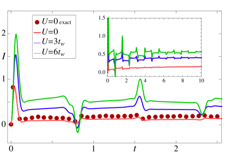
Figure 1: TD current for different $U$ at fixed $\lambda$, and initial QD occupancy $n_{d}=1$. For $U=0$, exact data from Ref. albrecht are also displayed (circles). The parameters are $\lambda=16$, $\omega_{0}=8$, $V=26$, $\tilde{\epsilon}_{d}=-10$, $\Lambda=100$. Units: $10^{-1}\Gamma/2$ for energies and $(\Gamma/2)^{-1}$ for times. Inset: $I(t)$ for long propagation times (no within reach of current numerical techniques).

Transient regime.— From the solution of Eq. (9) we can extract the time-dependent (TD) QD density as well as the TD current $I_{\alpha}(t)$ at the $\alpha$ interface

$$I_{\alpha}(z)=\int d\bar{z}\,\Sigma_{\alpha}(z,\bar{z})G(\bar{z},z)+\mathrm{h.c.}\quad$$ (11)

We apply a symmetric bias $V_{L}=-V_{R}=V/2$ and calculate $I(t)=[I_{L}(t)+I_{R}(t)]/2$ for the parameters of Fig. 1. As anticipated the $U=0$ curve is almost on top of the diagrammatic Monte Carlo simulation albrecht . The TD current displays quasi-stationary plateaus between two consecutive times $2n\pi/\omega_{0}$; around these times we see sharp spikes. For $U>0$ we observe a significant enhancement of the current; the plateaus bend and the amplitude of the spikes increases. We understand this peculiar transient behavior by inspecting the self-energy in Eq. (10). In the top panel of Fig. (2) we plot $|\Sigma^{<}(t)|$ for increasing $\lambda$ at $U=0$. The effect of the ep interaction is twofold: an overall suppression proportional to $e^{-g}$ and a modulation of period $2\pi/\omega_{0}$ (coming from the double exponential $e^{e^{i\omega_{0}t}}$). Physically (see cartoon in the top panel of Fig. 2), if we start at time $t=T$ with one electron on the QD the phonon cloud is centered around the minumum at $x\simeq\lambda/\omega_{0}^{2}$ of the harmonic potential. The large $|\Sigma^{<}(T)|$ favors the transfer of the electron from the QD to the leads causing a sudden shift of the minumum to $x=0$. At this point the polaron (electron+cloud) cannot hop back to the QD since the overlap between the shifted phonon-cloud wavefunctions is negligible (small $|\Sigma^{<}(t)|$). Only after a dwelling time of order $2\pi/\omega_{0}$ this overlap is again sizable, the electron returns to the QD (large $|\Sigma^{<}(T+2\pi/\omega_{0})|$) and the cycle restarts. The physical interpretation offered by Eq. (10) enables us to explain the structure of the transient, how the system approaches the Franck-Condon blockade (FCB) regime and how screening effects change the picture.

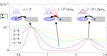
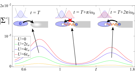
Figure 2: Modulus of the TD self-energy $|\Sigma^{<}_{\alpha}(t)|$ for different $\lambda$ at $U=0$ (top panel), and for different $U$ at $\lambda=8$ (bottom panel). The parameters are $\omega_{0}=8$, $\tilde{\epsilon}_{d}=0$ and $\Lambda=100$. Units: $\Lambda\Gamma$ for $|\Sigma^{<}|$, $\Gamma$ for energies and $\Gamma^{-1}$ for times.

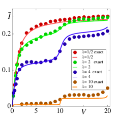
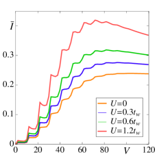
Figure 3: I-V curve for different $\lambda$ at $U=0$ (left panel), and for different $U$ at $\lambda=10$ (right panel). The parameters are $\omega_{0}=5$, $\tilde{\epsilon}_{d}=0$ and $\Lambda=1000$. For $U=0$ (left panel), exact data from Ref. rabani are also displayed (circles). All energies in units of $\Gamma$.

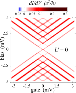
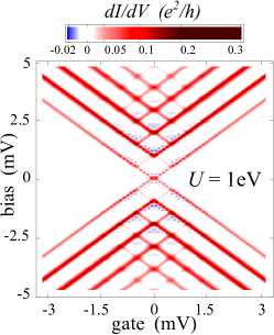
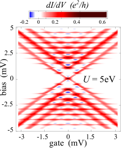
Figure 4: Contour plot of the differential conductance $dI/dV$ as a function of the gate $\tilde{\epsilon}_{d}$ and bias $V$, for three different the dot-lead repulsion: $U=0$ (left panel), $U=1$ eV (middle panel), $U=5$ eV (right panel). The rest of the parameters are specified in the text.

Indeed, a nonvanishing $U$ modifies the envelope of $|\Sigma^{<}|$ from the noninteracting power-law $1/t$ to $1/t^{\beta}$, see bottom panel of Fig. 2. According to the cartoon an electron in the QD causes a depletion of charge in the vicinity of the interface, thus facilitating the tunneling mahan ; borda ; goldstein ; irlm . Similarly, when the electron is in the leads the hole left on the QD acts as an attractive potential and the probability to tunnel back increases. This explains the enhancement of $I(t)$ in Fig. 1.

Steady-state.— In the steady-state regime $G$ and $\Sigma_{\alpha}$ depend only on the time difference and can be Fourier transformed. The steady current $\bar{I}$ is given by a Meir-Wingreen-like formula irlm ; wingreen

$$\bar{I}=\int\frac{d\omega}{2\pi}\frac{\Sigma^{>}_{L}(\omega)\Sigma^{<}_{R}(\omega)-\Sigma^{<}_{L}(\omega)\Sigma^{>}_{R}(\omega)}{|\omega-\tilde{\epsilon}_{d}-\sum_{\alpha}\Sigma_{\alpha}^{\rm R}(\omega)|^{2}},$$ (12)

where the explicit expression for the self-energy in frequency space is

$$\Sigma^{\lessgtr}_{\alpha}(\omega)=\pm i\frac{\Gamma e^{-g}}{2\Gamma(\beta)}\sum_{n=0}^{\infty}\frac{g^{n}}{n!}|\omega^{\lessgtr}_{\alpha n}/\Lambda|^{\beta-1}\theta(\pm\omega^{\lessgtr}_{\alpha n}),$$ (13)

with $\omega^{\lessgtr}_{\alpha n}=\omega\pm n\omega_{0}-V_{\alpha}$, $\Gamma(\beta)$ the Euler-Gamma function and $\theta$ the Heavyside step function nota2 .

In Fig. 3 we show the I-V curve for different $\lambda$ at $U=0$ (left panel), and for different $U$ at fixed $\lambda=10$ (right panel). The former is benchmarked against real-time path-integral Monte Carlo results rabani . Again we find good quantitative agreement from weak to strong coupling. The FCB suppression of $\bar{I}$ at large $\lambda$ as well as the phonon-assisted current steps at $V=2\omega_{0}$ are correctly reproduced. Turning on the ee interaction the Coulomb deblocking takes place and $\bar{I}$ increases for all $V$. We still observe phonon-assisted steps but, unexpectedly, they bend downward giving rise to regions of NDC. This phenomenon is our second main finding and is driven by the competition between ee and ep interactions (no NDC for $U=0$ or $\lambda=0$). By further increasing the bias a crossover occurs: the steps are attenuated and the current acquires a power-law decay $\bar{I}\sim V^{\beta-1}$. In this region the system behaves as if the ep coupling were zero boulat ; irlm .

NDC.— We investigate further the NDC aspect by calculating the $dI/dV$ as a function of voltage $V$ and gate $\tilde{\epsilon}_{d}$. NDC regions have been observed in QDs formed between the defects of a carbon nanotube (CNT) vonoppen . Even though theoretical studies have so far been focussed on the ep coupling vonoppen ; sassetti , the left/right portion of the CNT screens the charge accumulated on the QD. Our Hamiltonian represents the simplest generalization of previous models to include this screening effect. We use parameters from the literature: $\omega_{0}=1$ meV, $\lambda=1.82$ meV, $a=2.46$ Å, $v_{F}=8.1\times 10^{5}$ m/s, $\Gamma=0.1$ meV, and $\Lambda=0.1$ eV cntu . For the ee coupling we take $U<5$ eV, since in CNTs the on-site repulsion is $\sim 5$ eV auger . In Fig. 4 we show the contour plot of the $dI/dV$ for three different $U$s. The $U=0$ case accurately reproduces the FCB diamonds obtained within the rate equations approach fcb and later observed in experiments vonoppen . However, no signatures of NDC are found. For $U=1$ eV, instead, spots of NDC appear inside the diamonds, in qualitative agreeement with the experiment. Increasing $U$ even further the NDC regions expand, and horizontal stripes of large conductance emerge. However, these stripes should be suppressed by the strong, local repulsion (not considered here) responsible for the standard Coulomb blockade.

Conclusions.— We derived an approximate, yet accurate, formula for the electrical current through a QD with ep and ee coupling. Screening and polaronic features are transparently incorporated, rendering the physical interpretation direct and intuitive. The competition between FCB and Coulomb deblocking leads to the novel effect of NDC regions in the $dI/dV$. This mechanism occurs in QD weakly coupled to low-dimensional leads, like those recently realized with CNT.

We acknowledges funding by MIUR FIRB grant No. RBFR12SW0J.

References

- (1) M. Galperin, M.A. Ratner, A. Nitzan, and A. Troisi, Science 319, 1056 (2008).
- (2) J. Koch and F. J. von Oppen, Phys. Rev. Lett. 94, 206804 (2005).
- (3) R. Leturcq, C. Stampfer, K. Inderbitzin, L. Durrer, C. Hierold, E. Mariani, F. von Oppen and K. Ensslin, Nature Phys. 5, 327 (2009).
- (4) G. D. Mahan, Phys. Rev. Lett. 18, 448 (1967); P. Nozières, C.T. De Dominicis, Phys. Rev. 178 1097 (1969).
- (5) L. Borda, K. Vladár, and A. Zawadowski, Phys. Rev. B 70, 125107 (2007).
- (6) M. Goldstein, R. Berkovits, and Y. Gefen, Phys. Rev. Lett. 104, 226805 (2010).
- (7) E. Perfetto, G. Stefanucci and M. Cini, Phys. Rev. B 85, 165437 (2012).
- (8) L. Mühlbacher and E. Rabani, Phys. Rev. Lett. 100, 176403 (2008).
- (9) K. F. Albrecht, A. Martin-Rodero, R. C. Monreal, L. Mühlbacher, and A. Levy Yeyati, Phys. Rev. B 87, 085127 (2013).
- (10) E.Y. Wilner, H. Wang, G. Cohen, M. Thoss, E. Rabani, arXiv:1301.7681.
- (11) H. Wang and M. Thoss, J. Chem. Phys. 138, 134704 (2013).
- (12) F. Cavaliere, E. Mariani, R. Leturcq, C. Stampfer, and Maura Sassetti, Phys. Rev. B 81, 201303(R) (2010).
- (13) R. Härtle and M. Thoss, Phys. Rev. B 83, 115414 (2011).
- (14) M. Galperin, M.A. Ratner and A. Nitzan, NanoLett. 5, 125 (2005).
- (15) A. Zazunov, D. Feinberg, and T. Martin, Phys. Rev. B 73, 115405 (2006).
- (16) E. Boulat, H. Saleur, and P. Schmitteckert, Phys. Rev. Lett. 101, 140601 (2008).
- (17) T. Giamarchi, Quantum Physics in One Dimension (Clarendon, Oxford, 2004).
- (18) For the discrete and continuum version of yield the same results which, therefore, are independent of psc.2010 ; irlm .
- (19) E. Perfetto, G. Stefanucci and M. Cini, Phys. Rev. Lett. 105, 156802 (2010).
- (20) G. Stefanucci and R. van Leeuwen, Nonequilibrium Many- Body Theory of Quantum Systems: A Modern Introduction (Cambridge University Press, 2013).
- (21) We briefly discuss the differences with an alternative approach to deal with ep interactions () galperin . Our correlator between the fields is not dressed by virtual tunneling processes whereas in Ref. galperin this dressing is accounted for up to second-order in a self-consistent manner. However, in Ref. galperin the Green’s function satisfies Eq. (9) in which the under the integral sign is replaced by the noninteracting . Consequently the noninteracting case () is not recovered.
- (22) M. Galperin, A. Nitzan, and M.A. Ratner, Phys. Rev. B 73, 045314 (2006).
- (23) N. E. Dahlen and R. van Leeuwen, Phys. Rev. Lett. 98, 153004 (2007).
- (24) P. Myöhänen, A. Stan, G. Stefanucci and R. van Leeuwen, Phys. Rev. B 80, 115107 (2009).
- (25) N. S. Wingreen, K. W. Jacobsen, and J. W. Wilkins, Phys. Rev. B 40, 11834 (1989).
- (26) The retarded component of in Eq. (12) is extracted from .
- (27) J. González and E. Perfetto Phys. Rev. B 72, 205406 (2005); E. Perfetto and J. González, Phys. Rev. B 74, 201403 (2006).
- (28) E. Perfetto, M. Cini, S. Ugenti, P. Castrucci, M. Scarselli, M. De Crescenzi, F. Rosei, and M. A. El Khakani, Phys. Rev. B 76, 233408 (2007).