Quadrangulations with no pendant vertices

Abstract

We prove that the metric space associated with a uniformly distributed planar quadrangulation with $n$ faces and no pendant vertices converges modulo a suitable rescaling to the Brownian map. This is a first step towards the extension of recent convergence results for random planar maps to the case of graphs satisfying local constraints.

and

1 Introduction

Much recent work has been devoted to studying the convergence of rescaled planar graphs, viewed as metric spaces for the graph distance, towards the universal limiting object called the Brownian map. In the present article, we establish such a limit theorem in a particular instance of planar maps satisfying local constraints, namely quadrangulations with no pendant vertices, or equivalently with no vertices of degree $1$.

Recall that a planar map is a proper embedding of a finite connected graph in the two-dimensional sphere, considered up to orientation-preserving homeomorphisms of the sphere. Loops and multiple edges are a priori allowed (however in the case of bipartite graphs that we will consider, there cannot be any loop). The faces of the map are the connected components of the complement of edges, and the degree of a face counts the number of edges that are incident to it, with the convention that if both sides of an edge are incident to the same face, this edge is counted twice in the degree of the face (alternatively, the degree of a face may be defined as the number of corners to which it is incident). Let $p\geq 3$ be an integer. Special cases of planar maps are $p$-angulations (triangulations if $p=3$, or quadrangulations if $p=4$) where each face has degree $p$. For technical reasons, one often considers rooted planar maps, meaning that there is a distinguished oriented edge, whose tail vertex is called the root vertex. Planar maps have been studied thoroughly in combinatorics, and they also arise in other areas of mathematics. Large random planar graphs are of interest in theoretical physics, where they serve as models of random geometry [2], in particular in the theory of two-dimensional quantum gravity.

The recent paper [10] has established a general convergence theorem for rescaled random planar maps viewed as metric spaces. Let $p\geq 3$ be such that either $p=3$ or $p$ is even. For every integer $n\geq 1$, let ${\mathbf{m}}_{n}$ be a random planar map that is uniformly distributed over the set of all rooted $p$-angulations with $n$ faces (when $p=3$ we need to restrict our attention to even values of $n$ so that this set is not empty). We denote the vertex set of ${{\mathbf{m}}}_{n}$ by $V({\mathbf{m}}_{n})$. We equip $V({\mathbf{m}}_{n})$ with the graph distance ${\mathrm{d}}^{{\mathbf{m}}_{n}}_{\mathrm{gr}}$, and we view $(V({\mathbf{m}}_{n}),{\mathrm{d}}^{{\mathbf{m}}_{n}}_{\mathrm{gr}})$ as a random variable taking values in the space ${\mathbb{K}}$ of isometry classes of compact metric spaces. We equip ${\mathbb{K}}$ with the Gromov–Hausdorff distance $d_{GH}$ (see, e.g., [4]) and note that $({\mathbb{K}},d_{GH})$ is a Polish space. The main result of [10] states that there exists a random compact metric space $({\mathbf{m}}_{\infty},D^{*})$ called the Brownian map, which does not depend on $p$, and a constant $c_{p}>0$ depending on $p$, such that

$$\bigl{(}V({\mathbf{m}}_{n}),c_{p}n^{-1/4}{\mathrm{d}}^{{\mathbf{m}}_{n}}_{\mathrm{gr}}\bigr{)}\,\mathop{\longrightarrow}\limits_{n\to\infty}\limits^{(\mathrm{d})}\,\bigl{(}{\mathbf{m}}_{\infty},D^{*}\bigr{)}$$ (1)

where the convergence holds in distribution in the space $({\mathbb{K}},d_{GH})$. A precise description of the Brownian map is given below at the beginning of Section 3. The constants $c_{p}$ are known explicitly (see [10]) and in particular $c_{4}=(\frac{9}{8})^{1/4}$. We observe that the case $p=4$ of (1) has been obtained independently by Miermont [14], and that the case $p=3$ solves a question raised by Schramm [15]. Note that the first limit theorem involving the Brownian map was given in the case of quadrangulations by Marckert and Mokkadem [13], but in a weaker form than stated in (1).

In this work, we are interested in planar maps that satisfy additional local regularity properties. Under such constraints, one may ask whether the scaling limit is still the Brownian map, and, if it is, one expects to get different scaling constants $c_{p}$. Note that the general strategy for proving limiting results such as (1) involves coding the planar maps by certain labeled trees and deriving asymptotics for these trees. If the map is subject to local constraints, say concerning the degree of vertices, or the absence of multiple edges or of loops (in the case of triangulations), this leads to certain conditionings of the trees, which often make the desired asymptotics much harder to handle. In the present work, we consider quadrangulations with no pendant vertices, or equivalently with no vertices of degree $1$, which we call nice quadrangulations (see Figure 1). We let ${\mathcal{Q}}_{n}^{\mathrm{nice}}$ be the set of all rooted nice quadrangulations with $n$ faces. This set is nonempty for every $n\geq 2$.

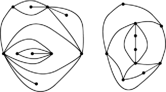
Figure 1: Two quadrangulations with $8$ faces. The one on the right is nice.

Theorem 1.1

For every $n\geq 2$, let ${\mathbf{q}}_{n}$ be uniformly distributed over the set ${\mathcal{Q}}_{n}^{\mathrm{nice}}$. Let $V({\mathbf{q}}_{n})$ be the vertex set of ${\mathbf{q}}_{n}$ and let ${\mathrm{d}}^{{\mathbf{q}}_{n}}_{\mathrm{gr}}$ be the graph distance on $V({\mathbf{q}}_{n})$. Then,

$$\bigl{(}V({\mathbf{q}}_{n}),\bigl{(}{\textstyle\frac{3}{4}}\bigr{)}^{3/8}n^{-1/4}{\mathrm{d}}^{{\mathbf{q}}_{n}}_{\mathrm{gr}}\bigr{)}\,\mathop{\longrightarrow}\limits_{n\to\infty}\limits^{(\mathrm{d})}\,\bigl{(}{\mathbf{m}}_{\infty},D^{*}\bigr{)}$$

where $({\mathbf{m}}_{\infty},D^{*})$ is the Brownian map, and the convergence holds in distribution in the space $({\mathbb{K}},d_{GH})$.

We observe that the limiting space is again the Brownian map, and so one may say that nice quadrangulations have asymptotically the same “shape” as ordinary quadrangulations. On the other hand, the scaling constant is different: Since $(\frac{3}{4})^{3/8}<(\frac{9}{8})^{1/4}$, distances are typically larger in nice quadrangulations, as one might have expected.

In relation with Theorem 1.1, we mention the recent work of Bouttier and Guitter [3], which obtains detailed information about distances in large quadrangulations with no multiple edges. Note that a quadrangulation with no multiple edges is always nice in our sense, but the converse is not true (see the nice quadrangulation on the right side of Figure 1).

We view Theorem 1.1 as a first step towards the derivation of similar results in more difficult cases. A particularly interesting problem is to derive the analog of (1) for triangulations without loops or multiple edges (type III triangulations in the terminology of [2]). It is known that such a triangulation can be represented as the tangency graph of a circle packing of the sphere, and that this representation is unique up to the conformal transformations of the sphere (the Möbius transformations). So assuming that the analog of (1) holds for type III triangulations, one might expect to be able to pass to the limit $n\to\infty$ in the associated circle packings, and to get a canonical embedding of the Brownian map in the sphere that would satisfy remarkable conformal invariance properties. One also conjectures that this canonical embedding would be related to the recent approach to two-dimensional quantum gravity which has been developed by Duplantier and Sheffield [6] via the Gaussian free field. The previous questions are among the most fascinating open problems in the area.

As a final remark, our proofs rely on Schaeffer’s bijection between rooted quadrangulations and well-labeled trees. One may be tempted to use the version of this bijection for rooted and pointed quadrangulations, which avoids the positivity condition on labels (see, e.g., [11]). However, the use of this other version of the bijection in our setting would lead to certain conditionings (involving the event that the minimal label on the tree is attained at two different corners), which seem difficult to handle.

The paper is organized as follows. In Section 2, we recall Schaeffer’s bijection (we refer to [5] for more details) and we identify those trees that correspond to nice triangulations. We then state the key limit theorem for the coding functions of the random tree associated with a uniformly distributed nice quadrangulation with $n$ faces. This limit theorem is the main ingredient of our proof of Theorem 1.1 in Section 3, which also uses some ideas introduced in [10] to deal with triangulations. The proof of the limit theorem for coding functions is given in Section 4, which is the most technical part of the paper.

2 Trees and quadrangulations

2.1 Labeled trees

We set ${\mathbb{N}}=\{1,2,\ldots\}$ and by convention ${\mathbb{N}}^{0}=\{\varnothing\}$. We introduce the set

$${\mathbb{V}}=\bigcup_{n=0}^{\infty}{\mathbb{N}}^{n}.$$

An element of ${\mathbb{V}}$ is thus a sequence $u=(u^{1},\ldots,u^{n})$ of elements of ${\mathbb{N}}$, and we set $|u|=n$, so that $|u|$ represents the “generation” of $u$. If $u=(u^{1},\ldots,u^{m})$ and $v=(v^{1},\ldots,v^{n})$ belong to $\mathcal{U}$, we write $uv=(u^{1},\ldots,u^{m},v^{1},\ldots,v^{n})$ for the concatenation of $u$ and $v$. In particular, $u\varnothing=\varnothing u=u$.

If $w\in{\mathbb{V}}$, we write ${\mathbb{V}}_{(w)}$ for the set of all elements $u\in{\mathbb{V}}$ of the form $u=wv$ for some $v\in{\mathbb{V}}$. We then set ${\mathbb{V}}^{(w)}=({\mathbb{V}}\setminus{\mathbb{V}}_{(w)})\cup\{w\}$.

The mapping $\pi:{\mathbb{V}}\setminus\{\varnothing\}\longrightarrow{\mathbb{V}}$ is defined by $\pi((u^{1},\ldots,u^{n}))=(u^{1},\ldots,u^{n-1})$ ($\pi(u)$ is the “parent” of $u$).

A plane tree $\tau$ is a finite subset of ${\mathbb{V}}$ such that:

1. [(iii)]

2. $\varnothing\in\tau$.

3. $u\in\tau\setminus\{\varnothing\}\Rightarrow\pi(u)\in\tau$.

4. For every $u\in\tau$, there exists an integer $k_{u}(\tau)\geq 0$ such that, for every $j\in{\mathbb{N}}$, $uj\in\tau$ if and only if $1\leq j\leq k_{u}(\tau)$.

Edges of $\tau$ are all pairs $(u,v)$ where $v\in\tau\setminus\{\varnothing\}$ and $u=\pi(v)$. We write $E(\tau)$ for the set of all edges of $\tau$. Every $e\in E(\tau)$ can therefore be written as $e=(e_{-},e_{+})$ where $e_{-}=\pi(e_{+})$. By definition, the size $|\tau|$ of $\tau$ is the number of edges of $\tau$, $|\tau|=\#E(\tau)=\#\tau-1$.

In what follows, we see each vertex of the tree $\tau$ as an individual of a population whose family tree is the tree $\tau$. In (iii) above, the individuals of the form $uj$, with $j\in{\mathbb{N}}$, are interpreted as the “children” of $u$, and they are ordered in the obvious way. The number $k_{u}(\tau)$ is the number of children of $u$ in $\tau$. The notions of an ancestor and a descendant of a vertex $u$ are defined similarly.

Let $\tau$ be a plane tree and $n=|\tau|$. The contour exploration sequence of $\tau$ is the finite sequence $v_{0},v_{1},\ldots,v_{2n}$ which is defined inductively as follows. First $v_{0}=\varnothing$, and then, for every $i\in\{0,\ldots,2n-1\}$, $v_{i+1}$ is either the first child of $v_{i}$ that does not appear among $v_{0},v_{1},\ldots,v_{i}$, or, if there is no such child, the parent of $v_{i}$. Informally, if the tree is embedded in the plane as suggested in Figure 2, we imagine the motion of a particle that starts from the root and traverses the tree from the left to the right, in the way explained by the arrows of Figure 2, until all edges have been explored and the particle has come back to the root. Then $v_{0},v_{1},\ldots,v_{2n}$ are the successive vertices visited by the particle. The contour function of the tree is defined by $C_{i}=|v_{i}|$ for every $i\in\{0,1,\ldots,2n\}$. We extend the function $C_{t}$ to the real interval $[0,2n]$ by linear interpolation, and by convention we set $C_{t}=0$ for $t\geq 2n$. Clearly the tree $\tau$ is determined by its contour function $(C_{t})_{t\geq 0}$.

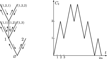
Figure 2: A plane tree with $n=7$ edges and its contour function.

A labeled tree is a pair $(\tau,(U(v))_{v\in\tau})$ that consists of a plane tree $\tau$ and a collection $(U(v))_{v\in\tau}$ of integer labels assigned to the vertices of $\tau$ – in our formalism for plane trees, the tree $\tau$ coincides with the set of all its vertices. We assume that labels satisfy the following three properties:

1. [(iii)]

2. for every $v\in\tau$, $U(v)\in{\mathbb{Z}}$;

3. $U(\varnothing)=0$;

4. for every $v\in\tau\setminus\{\varnothing\}$, $U(v)-U({\pi(v)})\in\{-1,0,1\}$,

where we recall that $\pi(v)$ denotes the parent of $v$. Condition (iii) just means that when crossing an edge of $\tau$ the label can change by at most $1$ in absolute value. We write ${\mathcal{W}}$ for the set of all labeled trees.

Let $(\tau,(U(v))_{v\in\tau})$ be a labeled tree with $n$ edges. As we have just seen, the plane tree $\tau$ is coded by its contour function $(C_{t})_{t\geq 0}$. We can similarly encode the labels by another function $(V_{t})_{t\geq 0}$, which is defined as follows. As above, let $v_{0},v_{1},v_{2},\ldots,v_{2n}$ be the contour exploration sequence of $\tau$. We set

$$V_{i}=U({v_{i}})\quad\mbox{for every }i=0,1,\ldots,2n.$$

Notice that $V_{0}=V_{2n}=0$. We extend the function $V_{t}$ to the real interval $[0,2n]$ by linear interpolation, and we set $V_{t}=0$ for $t\geq 2n$. We will call $(V_{t})_{t\geq 0}$ the “label function” of the labeled tree $(\tau,(U(v))_{v\in\tau})$. Clearly $(\tau,(U(v))_{v\in\tau})$ is determined by the pair $(C_{t},V_{t})_{t\geq 0}$.

We write ${\mathcal{W}}^{+}$ for the set of all labeled trees with nonnegative labels (these are sometimes called well-labeled trees), and for every $n\geq 0$, we write ${\mathcal{W}}^{+}_{n}$ for the set of all labeled trees with $n$ edges in ${\mathcal{W}}^{+}$.

2.2 Schaeffer’s bijection

In this section, we fix $n\geq 1$ and we briefly recall Schaeffer’s bijection between the set ${\mathcal{Q}}_{n}$ of all rooted quadrangulations with $n$ faces and the set ${\mathcal{W}}^{+}_{n}$. We refer to [5] for more details. We then characterize those labeled trees that correspond to nice quadrangulations in this bijection.

To describe Schaeffer’s bijection, start from a labeled tree $(\tau,(U(v))_{v\in\tau})\in{\mathcal{W}}^{+}_{n}$, and as above write $v_{0},v_{1},v_{2},\ldots,v_{2n}$ for the contour exploration sequence of the vertices of $\tau$. Notice that each index $i\in\{0,1,\ldots,2n-1\}$ corresponds to exactly one corner of the vertex $v_{i}$ (a corner of a vertex $v$ of $\tau$ is an angular sector between two successive edges of $\tau$ around the vertex $v$). This corner will be called the corner $i$ in the tree $\tau$.

We extend the contour exploration sequence periodically, in such a way that $v_{i+2n}=v_{i}$ for every integer $i\geq 0$. Then, for every $i\in\{0,1,\ldots,2n-1\}$, we define the successor of $i$ by setting

$${\mathrm{succ}}(i)=\cases{\min\bigl{\{}j\geq i:U(v_{j})=U(v_{i})-1\bigr{\}},&if $U(v_{i})>0$,\cr\infty,&otherwise.}$$

To construct the edges of the quadrangulation associated with $(\tau,(U(v))_{v\in\tau})$, we proceed in the following way. We suppose that the tree $\tau$ is drawn in the plane in the way suggested in Figure 2, and we add an extra vertex $\partial$ (outside the tree). Then, for every $i\in\{0,1,\ldots,2n-1\}$,

1. Either $U(v_{i})=0$, and we draw an edge between $v_{i}$ and $\partial$, that starts from the corner $i$.

2. Or $U(v_{i})>0$, and we draw an edge between $v_{i}$ and $v_{{\mathrm{succ}}(i)}$, that starts from the corner $i$ and ends at the corner ${\mathrm{succ}}(i)$.

The construction can be made in such a way that the edges do not intersect, and do not intersect the edges of the tree (see Figure 3 for an example). The resulting graph, whose vertex set consists of all vertices of $\tau$ and the vertex $\partial$, is a quadrangulation with $n$ faces. It is rooted at the edge drawn between the vertex $\varnothing$ of $\tau$ and the vertex $\partial$, which is oriented in such a way that $\partial$ is the root vertex. We have thus obtained a rooted quadrangulation with $n$ faces, which is denoted by ${\mathbf{q}}=\Phi_{n}(\tau,(U(v))_{v\in\tau})$. The mapping $\Phi_{n}$ is Schaeffer’s bijection from ${\mathcal{W}}^{+}_{n}$ onto ${\mathcal{Q}}_{n}$. A key property of this bijection is the fact that labels on the tree $\tau$ become distances from the root vertex $\partial$ in the quadrangulation: If ${\mathrm{d}}^{\mathbf{q}}_{\mathrm{gr}}$ stands for the graph distance on the vertex set of ${\mathbf{q}}$, we have

$${\mathrm{d}}^{\mathbf{q}}_{\mathrm{gr}}(\partial,v)=U(v)+1,$$

for every vertex $v$ of $\tau$ or equivalently for every vertex $v$ of ${\mathbf{q}}$ other than the root vertex.

Figure 3: Illustration of Schaeffer’s bijection. The thin lines represent the edges of the tree, and the numbers $0,1,\ldots$ are the labels assigned to the different vertices. The thick curves represent the edges of the associated quadrangulation. The two pendant vertices are the leaves $v$ such that $U(v)\geq U(\pi(v))$.

A leaf of the tree $\tau$ is a vertex with degree $1$. If $v\in\tau\setminus\{\varnothing\}$, $v$ is a leaf if and only if $k_{v}(\tau)=0$, and $\varnothing$ is a leaf if and only if $k_{\varnothing}(\tau)=1$.

Proposition 2.1

Let $(\tau,(U(v))_{v\in\tau})\in{\mathcal{W}}^{+}_{n}$, and let $v_{0},v_{1},\ldots,v_{2n}$ be the contour exploration sequence of $\tau$. Then the quadrangulation $\Phi_{n}(\tau,(U(v))_{v\in\tau})$ is nice if and only if the following two conditions hold.

1. [(ii)]

2. For every leaf $v$ of $\tau$, if $w$ is the (unique) vertex adjacent to $v$ in the tree $\tau$, we have $U(v)=U(w)-1$.

3. There exists at least one index $i\in\{1,\ldots,2n-1\}$ such that $U(v_{i})=0$.

Notice that we have always $U(v_{0})=U(\varnothing)=0$. Condition (ii) can be restated by saying that there are at least two corners of the tree $\tau$ with label $0$. In particular this condition holds if $k_{\varnothing}(\tau)\geq 2$.

Proof of Proposition 2.1 Let us explain why conditions (i) and (ii) are necessary. If (ii) does not hold, there is only one edge incident to $\partial$. If there exists a leaf $v$ for which the property stated in (i) fails, then the only edge incident to $v$ will be the edge connecting the unique corner of $v$ to its successor. Conversely, it is also very easy to check that if conditions (i) and (ii) hold then every vertex of $\tau$ will be incident to at least $2$ edges in the quadrangulation $\Phi_{n}(\tau,(U(v))_{v\in\tau})$: In particular if $v$ is a leaf of $\tau$ and if $w$ is the vertex adjacent to $v$, then the successor of one of the corners of $w$ will be the (unique) corner of $v$. We leave the details to the reader.

Remark 2.2.

For a general quadrangulation, each leaf $v\neq\varnothing$ of the associated labeled tree such that $U(v)\geq U(\pi(v))$ corresponds to a pendant vertex (see Figure 3). Using this observation, it is not hard to prove that a quadrangulation with $n$ faces has typically about $n/3$ pendant vertices.

We write ${\mathcal{W}}^{\mathrm{nice}}_{n}$ for the set of all labeled trees in ${\mathcal{W}}^{+}_{n}$ that satisfy both conditions in Proposition 2.1.

2.3 Scaling limits for coding functions

In this section, we state the key theorem giving scaling limits for the contour and label functions of the labeled tree associated with a uniformly distributed nice quadrangulation with $n$ faces. We first need to introduce the limiting processes that will appear in this theorem.

We let ${\mathbf{e}}=({\mathbf{e}}_{t})_{t\in[0,1]}$ denote a normalized Brownian excursion. The process ${\mathbf{e}}$ is defined on a probability space $(\Omega,\mathcal{A},{\mathbb{P}})$. We consider another real-valued process $Z=(Z_{t})_{t\in[0,1]}$ defined on the same probability space and such that, conditionally on ${\mathbf{e}}$, $Z$ is a centered Gaussian process with covariance

$${{\mathbb{E}}}[Z_{s}Z_{t}\mid{\mathbf{e}}]=\min_{r\in[s\wedge t,s\vee t]}{\mathbf{e}}_{r}.$$

We may and will assume that $Z$ has continuous sample paths. The process $Z$ can be interpreted as the head of the standard Brownian snake driven by ${\mathbf{e}}$.

It is not hard to verify that the distribution of

$$\min_{t\in[0,1]}Z_{t}$$

has no atoms, and that the topological support of this distribution is $(-\infty,0]$. Consequently, we can consider for every $r>0$ a process $({\mathbf{e}}^{(r)},Z^{(r)})$ whose distribution is the conditional distribution of $({\mathbf{e}},Z)$ knowing that

$$\min_{t\in[0,1]}Z_{t}>-r,$$

and the distribution of $({\mathbf{e}}^{(r)},Z^{(r)})$ depends continuously on $r>0$. Here the distribution of $({\mathbf{e}}^{(r)},Z^{(r)})$ is a probability measure on the space $C([0,1],{\mathbb{R}}^{2})$ of all continuous functions from $[0,1]$ into ${\mathbb{R}}^{2}$, and “continuously” refers to the usual weak convergence of probability measures. It is proved in [12], Theorem 1.1, that we can define a process $({\mathbf{e}}^{(0)},Z^{(0)})$ such that

$$\bigl{(}{\mathbf{e}}^{(r)},Z^{(r)}\bigr{)}\,\mathop{\longrightarrow}\limits_{r\to 0}\limits^{(\mathrm{d})}\,\bigl{(}{\mathbf{e}}^{(0)},Z^{(0)}\bigr{)}$$

where the convergence holds in distribution in the space $C([0,1],{\mathbb{R}}^{2})$.

The following theorem is the key ingredient of the proof of our main result.

Theorem 2.3

Let $C^{(n)}$ and $V^{(n)}$ be, respectively, the contour function and the label function of a random labeled tree distributed uniformly over ${\mathcal{W}}^{\mathrm{nice}}_{n}$. Then,

$$\bigl{(}12^{-1/4}n^{-1/2}C^{(n)}_{2nt},\bigl{(}{\textstyle\frac{3}{4}}\bigr{)}^{3/8}n^{-1/4}V^{(n)}_{2nt}\bigr{)}_{0\leq t\leq 1}\,\mathop{\longrightarrow}\limits_{n\to\infty}\limits^{(\mathrm{d})}\,\bigl{(}{\mathbf{e}}^{(0)}_{t},Z^{(0)}_{t}\bigr{)}_{0\leq t\leq 1},$$

where the convergence holds in distribution in $C([0,1],{\mathbb{R}}^{2})$.

The proof of Theorem 2.3 is given in Section 4 below.

3 Proof of the main theorem

In this section, we explain how to derive Theorem 1.1 from the convergence of coding functions stated in Theorem 2.3. Much of what follows is similar to the arguments of [9], Section 3, or of [11], Section 6.2, but we will provide some details for the sake of completeness.

We start by recalling the definition of the Brownian map. The first ingredient is the Continuum Random Tree or CRT, which is conveniently defined as the tree coded by the Brownian excursion (Aldous [1]). Recall that if $g:[0,1]\longrightarrow{\mathbb{R}}_{+}$ is a continuous function such that $g(0)=g(1)=0$, one introduces the equivalence relation on $[0,1]$ defined by

$$s\sim_{g}t\quad\mbox{if and only if}\quad g(s)=g(t)=m_{g}(s,t),$$

where $m_{g}(s,t)=\min\{g(r):s\wedge t\leq r\leq s\vee t\}$, and the tree coded by $g$ is the quotient space ${\mathcal{T}}_{g}:=[0,1]/\sim_{g}$, which is equipped with the distance induced by the pseudo-metric

$$\delta_{g}(s,t)=g(s)+g(t)-2m_{g}(s,t),\quad s,t\in[0,1].$$

We write $p_{g}:[0,1]\longrightarrow{\mathcal{T}}_{g}$ for the canonical projection. By convention, ${\mathcal{T}}_{g}$ is rooted at $p_{g}(0)=p_{g}(1)$. The CRT ${\mathcal{T}}_{\mathbf{e}}$ is then the (random) tree coded by the normalized Brownian excursion ${\mathbf{e}}$.

From the definition of the process $Z$, one easily checks that ${\mathbb{E}}[(Z_{s}-Z_{t})^{2}\mid{\mathbf{e}}]=\delta_{\mathbf{e}}(s,t)$, and it follows that we have $Z_{s}=Z_{t}$ for every $s,t\in[0,1]$ such that $s\sim_{\mathbf{e}}t$, a.s. Hence we may and sometimes will view $Z$ as indexed by ${\mathcal{T}}_{\mathbf{e}}$ rather than by $[0,1]$. For $a\in{\mathcal{T}}_{\mathbf{e}}$, we interpret $Z_{a}$ as the “label” of the vertex $a$.

We now explain how a trajectorial transformation of $({\mathbf{e}},Z)$ yields a pair $(\overline{\mathbf{e}},\overline{Z})$ having the same distribution as $({\mathbf{e}}^{(0)},Z^{(0)})$. By [12], Proposition 2.5 (and an obvious scaling argument) there exists an a.s. unique time $s_{*}\in[0,1]$ such that $Z_{s_{*}}=\min\{Z_{s}:s\in[0,1]\}$. We then set, for every $t\in[0,1]$,

$$\overline{\mathbf{e}}_{t} = \delta_{\mathbf{e}}(s_{*},s_{*}\oplus t)={\mathbf{e}}_{s_{*}}+{\mathbf{e}}_{s_{*}\oplus t}-2m_{\mathbf{e}}(s_{*},s_{*}\oplus t),$$

$$\overline{Z}_{t} = Z_{s_{*}\oplus t}-Z_{s_{*}},$$

where $s_{*}\oplus t=s+t$ if $s_{*}+t\leq 1$ and $s_{*}\oplus t=s+t-1$ otherwise. By [12], Theorem 1.2, the pair $(\overline{\mathbf{e}},\overline{Z})$ has the same distribution as $({\mathbf{e}}^{(0)},Z^{(0)})$.

One easily verifies that the property $s_{*}\oplus t\sim_{{\mathbf{e}}}s_{*}\oplus t^{\prime}$ holds if and only if $t\sim_{\overline{\mathbf{e}}}t^{\prime}$, for every $t,t^{\prime}\in[0,1]$, a.s., and it follows that we have $\overline{Z}_{t}=\overline{Z}_{t^{\prime}}$ if $t\sim_{\overline{\mathbf{e}}}t^{\prime}$. Hence, we may again view $\overline{Z}$ as indexed by the tree ${\mathcal{T}}_{\overline{\mathbf{e}}}$.

The mapping $t\longrightarrow s_{*}\oplus t$ induces an isometry $\mathcal{I}$ from ${\mathcal{T}}_{\overline{\mathbf{e}}}$ onto ${\mathcal{T}}_{\mathbf{e}}$, that maps the root of ${\mathcal{T}}_{\overline{\mathbf{e}}}$ to the vertex $p_{\mathbf{e}}(s_{*})$ with minimal label in ${\mathcal{T}}_{\mathbf{e}}$. Furthermore, we have $\overline{Z}_{a}=Z_{\mathcal{I}(a)}-\min Z$ for every $a\in{\mathcal{T}}_{\overline{\mathbf{e}}}$. To summarize the preceding discussion, ${\mathcal{T}}_{\overline{\mathbf{e}}}$ can be viewed as ${\mathcal{T}}_{\mathbf{e}}$ “re-rooted” at the vertex with minimal label, and the labels $\overline{Z}$ on ${\mathcal{T}}_{\overline{\mathbf{e}}}$ are derived from the labels $Z$ on ${\mathcal{T}}_{\mathbf{e}}$ by subtracting the minimal label.

Next, for every $s,t\in[0,1]$, we set

$$D^{\circ}(s,t):=\overline{Z}_{s}+\overline{Z}_{t}-2\min_{s\wedge t\leq r\leq s\vee t}\overline{Z}_{r}$$

and, for every $a,b\in{\mathcal{T}}_{\overline{\mathbf{e}}}$,

$$D^{\circ}(a,b):=\inf\bigl{\{}D^{\circ}(s,t):s,t\in[0,1],p_{\overline{\mathbf{e}}}(s)=a,p_{\overline{\mathbf{e}}}(t)=b\bigr{\}}.$$

Finally, we define a pseudo-metric $D^{*}$ on ${\mathcal{T}}_{\overline{\mathbf{e}}}$ by setting

$$D^{*}(a,b):=\inf\Biggl{\{}\sum_{i=1}^{k}D^{\circ}(a_{i-1},a_{i})\Biggr{\}}$$

where the infimum is over all choices of the integer $k\geq 1$ and of the finite sequence $a_{0},a_{1},\ldots,a_{k}$ such that $a_{0}=a$ and $a_{k}=b$. We set $a\approx b$ if and only if $D^{*}(a,b)=0$ (according to [9], Theorem 3.4, this holds if and only if $D^{\circ}(a,b)=0$).

The Brownian map is the quotient space ${\mathbf{m}}_{\infty}:={\mathcal{T}}_{\overline{\mathbf{e}}}/\approx$, which is equipped with the distance induced by $D^{*}$. The reader may have noticed that our presentation is consistent with [9], but slightly differs from the introduction of [10], where the Brownian map is constructed directly from the pair $({\mathbf{e}},Z)$, rather than from $(\overline{\mathbf{e}},\overline{Z})$. The previous discussion about the relations between the trees ${\mathcal{T}}_{\mathbf{e}}$ and ${\mathcal{T}}_{\overline{\mathbf{e}}}$, and the labels on these trees, however shows that both presentations are equivalent. In the present work, because our limit theorem for the coding functions of discrete objects involves a pair distributed as $(\overline{\mathbf{e}},\overline{Z})$, it will be more convenient to use the presentation above.

Let us turn to the proof of Theorem 1.1. We let $(\tau_{n},(U_{n}(v))_{v\in{\mathbf{q}}_{n}})$ be the labeled tree associated with ${\mathbf{q}}_{n}$, which is uniformly distributed over ${\mathcal{W}}_{n}^{\mathrm{nice}}$. As in Theorem 2.3, we denote the contour function and the label function of $(\tau_{n},(U_{n}(v))_{v\in{\mathbf{q}}_{n}})$ by $C^{(n)}$ and $V^{(n)}$, respectively. We also write $u^{n}_{0},u^{n}_{1},\ldots,u^{n}_{2n}$ for the contour exploration sequence of $\tau_{n}$. We then set, for every $i,j\in\{0,1,\ldots,2n\}$,

$${\mathrm{d}}_{n}(i,j)={\mathrm{d}}^{{\mathbf{q}}_{n}}_{\mathrm{gr}}\bigl{(}u^{n}_{i},u^{n}_{j}\bigr{)}$$

where ${\mathrm{d}}^{{\mathbf{q}}_{n}}_{\mathrm{gr}}$ stands for the graph distance on $V({\mathbf{q}}_{n})$ (here and in what follows, we use Schaeffer’s bijection to view the vertices of $\tau_{n}$ as vertices of ${\mathbf{q}}_{n}$). We extend the definition of ${\mathrm{d}}_{n}(i,j)$ to noninteger values of $i$ and $j$ by setting, for every $s,t\in[0,2n]$,

$${\mathrm{d}}_{n}(s,t) = \bigl{(}s-\lfloor s\rfloor\bigr{)}\bigl{(}t-\lfloor t\rfloor\bigr{)}{\mathrm{d}}_{n}\bigl{(}\lceil s\rceil,\lceil t\rceil\bigr{)}+\bigl{(}s-\lfloor s\rfloor\bigr{)}\bigl{(}\lceil t\rceil-t\bigr{)}{\mathrm{d}}_{n}\bigl{(}\lceil s\rceil,\lfloor t\rfloor\bigr{)}$$

$${}+\bigl{(}\lceil s\rceil-s\bigr{)}\bigl{(}t-\lfloor t\rfloor\bigr{)}{\mathrm{d}}_{n}\bigl{(}\lfloor s\rfloor,\lceil t\rceil\bigr{)}+\bigl{(}\lceil s\rceil-s\bigr{)}\bigl{(}\lceil t\rceil-t\bigr{)}{\mathrm{d}}_{n}\bigl{(}\lfloor s\rfloor,\lfloor t\rfloor\bigr{)},$$

where $\lceil t\rceil:=\min\{k\in{\mathbb{Z}}:k>t\}$. The same arguments as in [9], Proposition 3.2, relying on the bound

$${\mathrm{d}}_{n}(i,j)\leq V^{(n)}_{i}+V^{(n)}_{i}-2\min_{i\wedge i\leq k\leq i\vee j}V^{(n)}_{k}+2$$ (2)

(see [9], Lemma 3.1) and on Theorem 2.3 show that the sequence of the laws of the processes $(n^{-1/4}{\mathrm{d}}_{n}(2ns,2nt))_{0\leq s,t\leq 1}$ is tight in the space of all probability measures on $C([0,1]^{2},{\mathbb{R}}_{+})$. Using this tightness property and Theorem 2.3, we can find a sequence of integers $(n_{k})_{k\geq 1}$ converging to $+\infty$ and a continuous random process $(D(s,t))_{0\leq s\leq t}$ such that, along the sequence $(n_{k})_{k\geq 1}$, we have the joint convergence in distribution in $C([0,1]^{2},{\mathbb{R}}^{3})$,

$$\bigl{(}12^{-1/4}n^{-1/2}C^{(n)}_{2nt},\bigl{(}{\textstyle\frac{3}{4}}\bigr{)}^{3/8}n^{-1/4}V^{(n)}_{2nt},\bigl{(}{\textstyle\frac{3}{4}}\bigr{)}^{3/8}n^{-1/4}{\mathrm{d}}_{n}(2ns,2nt)\bigr{)}_{0\leq s,t\leq 1}$$ (3)

$$\quad\,\mathop{\longrightarrow}\limits_{n\to\infty}\limits^{(\mathrm{d})}\,\bigl{(}\overline{\mathbf{e}}_{t},\overline{Z}_{t},D(s,t)\bigr{)}_{0\leq s,t\leq 1}.$$

By Skorokhod’s representation theorem, we may assume that this convergence holds a.s. Passing to the limit $n\to\infty$ in (2), we get that $D(s,t)\leq D^{\circ}(s,t)$ for every $s,t\in[0,1]$, a.s. Also, from the fact that ${\mathrm{d}}^{{\mathbf{q}}_{n}}_{\mathrm{gr}}(\partial,u^{n}_{i})=U(u^{n}_{i})+1=V^{(n)}_{i}+1$ we immediately obtain that $D(0,t)=\overline{Z}_{t}$ for every $t\in[0,1]$, a.s.

Clearly, the function $(s,t)\longrightarrow D(s,t)$ is symmetric, and it also satisfies the triangle inequality because ${\mathrm{d}}_{n}$ does. Furthermore, the fact that ${\mathrm{d}}_{n}(i,j)=0$ if $u^{n}_{i}=u^{n}_{j}$ easily implies that $D(s,t)=0$ for every $s,t\in[0,1]$ such that $s\sim_{\overline{\mathbf{e}}}t$, a.s. (see the proof of Proposition 3.3(iii) in [9]). Hence, we may view $D$ as a random pseudo-metric on ${\mathcal{T}}_{\overline{\mathbf{e}}}$. Since $D\leq D^{\circ}$ and $D$ satisfies the triangle inequality, the definition of $D^{*}$ immediately shows that $D(a,b)\leq D^{*}(a,b)$ for every $a,b\in{\mathcal{T}}_{\overline{\mathbf{e}}}$, a.s.

Lemma 3.1

We have $D(a,b)=D^{*}(a,b)$ for every $a,b\in{\mathcal{T}}_{\overline{\mathbf{e}}}$, a.s.

We postpone the proof of Lemma 3.1 to the end of the section and complete the proof of Theorem 1.1. We define a correspondence between the metric spaces $(V({\mathbf{q}}_{n})\setminus\{\partial\},(\frac{3}{4})^{3/8}n^{-1/4}{\mathrm{d}}^{{\mathbf{q}}_{n}}_{\mathrm{gr}})$ and $({\mathbf{m}}_{\infty},D^{*})$ by setting

$${{\mathcal{R}}}_{n}:=\bigl{\{}\bigl{(}u^{n}_{\lfloor 2nt\rfloor},\Pi\bigl{(}p_{\overline{\mathbf{e}}}(t)\bigr{)}\bigr{)}:t\in[0,1]\bigr{\}}$$

where $\Pi$ stands for the canonical projection from ${\mathcal{T}}_{\overline{\mathbf{e}}}$ onto ${\mathbf{m}}_{\infty}$. The distortion of this correspondence is

$$\sup_{0\leq s,t\leq 1}\biggl{|}\biggl{(}\frac{3}{4}\biggr{)}^{3/8}n^{-1/4}{\mathrm{d}}^{{\mathbf{q}}_{n}}_{\mathrm{gr}}\bigl{(}u^{n}_{\lfloor 2ns\rfloor},u^{n}_{\lfloor 2nt\rfloor}\bigr{)}-D^{*}\bigl{(}p_{\overline{\mathbf{e}}}(s),p_{\overline{\mathbf{e}}}(t)\bigr{)}\biggr{|}$$

$$\quad=\sup_{0\leq s,t\leq 1}\biggl{|}\biggl{(}\frac{3}{4}\biggr{)}^{3/8}n^{-1/4}{\mathrm{d}}_{n}\bigl{(}\lfloor 2ns\rfloor,\lfloor 2nt\rfloor\bigr{)}-D(s,t)\biggr{|}$$

using Lemma 3.1 to write $D^{*}(p_{\overline{\mathbf{e}}}(s),p_{\overline{\mathbf{e}}}(t))=D(p_{\overline{\mathbf{e}}}(s),p_{\overline{\mathbf{e}}}(t))=D(s,t)$. From the (almost sure) convergence (3), the quantity in the last display tends to $0$ as $n\to\infty$ along the sequence $(n_{k})_{k\geq 1}$. From the expression of the Gromov–Hausdorff distance in terms of correspondences [4], Theorem 7.3.25, we conclude that

$$\bigl{(}V({\mathbf{q}}_{n})\setminus\{\partial\},\bigl{(}{\textstyle\frac{3}{4}}\bigr{)}^{3/8}n^{-1/4}{\mathrm{d}}^{{\mathbf{q}}_{n}}_{\mathrm{gr}}\bigr{)}\,\mathop{\longrightarrow}\limits\limits^{\mathrm{a.s.}}\,\bigl{(}{\mathbf{m}}_{\infty},D^{*}\bigr{)}$$

as $n\to\infty$ along the sequence $(n_{k})_{k\geq 1}$. Clearly, the latter convergence also holds if we replace $V({\mathbf{q}}_{n})\setminus\{\partial\}$ by $V({\mathbf{q}}_{n})$.

The preceding arguments show that from any sequence of integers converging to $\infty$ we can extract a subsequence along which the convergence of Theorem 1.1 holds. This is enough to prove Theorem 1.1.

Proof of Lemma 3.1 Here we follow the ideas of the treatment of triangulations in [10], Section 8. By a continuity argument, it is enough to prove that if $X$ and $Y$ are independent and uniformly distributed over $[0,1]$, and independent of the sequence $({\mathbf{q}}_{n})_{n\geq 1}$ (and therefore also of $({\mathbf{e}},Z,D)$), we have

$$D\bigl{(}p_{\overline{\mathbf{e}}}(X),p_{\overline{\mathbf{e}}}(Y)\bigr{)}=D^{*}\bigl{(}p_{\overline{\mathbf{e}}}(X),p_{\overline{\mathbf{e}}}(Y)\bigr{)}\quad\mbox{a.s.}$$

As we already know that $D(p_{\overline{\mathbf{e}}}(X),p_{\overline{\mathbf{e}}}(Y))\leq D^{*}(p_{\overline{\mathbf{e}}}(X),p_{\overline{\mathbf{e}}}(Y))$, it will be sufficient to prove that these two random variables have the same distribution. The distribution of $D^{*}(p_{\overline{\mathbf{e}}}(X),p_{\overline{\mathbf{e}}}(Y))$ is identified in Corollary 7.3 of [10]:

$$D^{*}\bigl{(}p_{\overline{\mathbf{e}}}(X),p_{\overline{\mathbf{e}}}(Y)\bigr{)}\,\mathop{=}\limits\limits^{(\mathrm{d})}\,Z_{X}-\min Z\,\mathop{=}\limits\limits^{(\mathrm{d})}\,\overline{Z}_{X}.$$

On the other hand, we can also derive the distribution of $D(p_{\overline{\mathbf{e}}}(X),p_{\overline{\mathbf{e}}}(Y))=D(X,Y)$. For every $n\geq 1$, we set

$$i_{n}=\lfloor 2nX\rfloor,\quad j_{n}=\lfloor 2nY\rfloor,$$

so that $i_{n}$ and $j_{n}$ are independent (and independent of ${\mathbf{q}}_{n}$) and uniformly distributed over $\{0,1,\ldots,2n-1\}$. Recall that every integer $i\in\{0,1,\ldots,2n-1\}$ corresponds to a corner of the tree $\tau_{n}$ and therefore via Schaeffer’s bijection to an edge of ${\mathbf{q}}_{n}$. We define $\widetilde{\mathbf{q}}_{n}$ by saying that $\widetilde{\mathbf{q}}_{n}$ is the same planar map as ${\mathbf{q}}_{n}$ but re-rooted at the edge associated with $i_{n}$, with each of the two possible orientations chosen with probability $\frac{1}{2}$. Then $\widetilde{\mathbf{q}}_{n}$ is also uniformly distributed over ${\mathcal{Q}}_{n}^{\mathrm{nice}}$, and we let $\widetilde{\tau}_{n}$ be the associated tree in Schaeffer’s bijection. Write $\widetilde{\mathrm{d}}_{n}$ for the analog of ${\mathrm{d}}_{n}$ when ${\mathbf{q}}_{n}$ is replaced by $\widetilde{\mathbf{q}}_{n}$.

Let $k_{n}\in\{0,1,\ldots,2n-1\}$ be the index of the corner of the tree $\widetilde{\tau}_{n}$ corresponding to the edge of ${\mathbf{q}}_{n}$ that starts from the corner $j_{n}$ of $\tau_{n}$ in Schaeffer’s bijection. Note that, conditionally on the pair $({\mathbf{q}}_{n},\widetilde{\mathbf{q}}_{n})$, the latter edge is uniformly distributed over all edges of ${\mathbf{q}}_{n}$, and is thus also uniformly distributed over all edges of $\widetilde{\mathbf{q}}_{n}$ (recall that $\widetilde{\mathbf{q}}_{n}$ is the same quadrangulation as ${\mathbf{q}}_{n}$ with a different root). Hence, conditionally on the pair $({\mathbf{q}}_{n},\widetilde{\mathbf{q}}_{n})$, $k_{n}$ is uniformly distributed over $\{0,1,\ldots,2n-1\}$, and in particular the random variable $k_{n}$ is independent of $\widetilde{\mathbf{q}}_{n}$. We next observe that

$$\bigl{|}{\mathrm{d}}_{n}(i_{n},j_{n})-\widetilde{\mathrm{d}}_{n}(0,k_{n})\bigr{|}\leq 2,$$ (4)

because, with an obvious notation, the vertex $u^{n}_{i_{n}}$ is either equal or adjacent to $\widetilde{u}^{n}_{0}$, and similarly $u^{n}_{j_{n}}$ is either equal or adjacent to $\widetilde{u}^{n}_{k_{n}}$.

Now we have $\widetilde{\mathrm{d}}_{n}(0,k_{n})\,\mathop{=}\limits\limits^{(\mathrm{d})}\,{\mathrm{d}}_{n}(0,i_{n})$ and by (3),

$$\bigl{(}{\textstyle\frac{3}{4}}\bigr{)}^{3/8}n^{-1/4}{\mathrm{d}}_{n}(0,i_{n})\,\mathop{\longrightarrow}\limits_{n\to\infty}\limits^{\mathrm{a.s.}}\,D(0,X)=\overline{Z}_{X}$$

where the convergence holds a.s. along the sequence $(n_{k})_{k\geq 1}$. Similarly, (3) implies that, along the same sequence,

$$\bigl{(}{\textstyle\frac{3}{4}}\bigr{)}^{3/8}n^{-1/4}{\mathrm{d}}_{n}(i_{n},j_{n})\,\mathop{\longrightarrow}\limits_{n\to\infty}\limits^{\mathrm{a.s.}}\,D(X,Y).$$

From the last two convergences and (4), we obtain that $D(X,Y)$ has the same distribution as $\overline{Z}_{X}$. Since we already observed that this is also the distribution of $D^{*}(p_{\overline{\mathbf{e}}}(X),p_{\overline{\mathbf{e}}}(Y))$, the proof of the lemma is complete.

4 The convergence of coding functions

In this section, we prove our main technical result Theorem 2.3. We start by deriving an intermediate convergence theorem.

4.1 A preliminary convergence

If $\tau$ is a plane tree, we let $\partial\tau$ stand for the set of all leaves of $\tau$ different from the root vertex (which may or may not be a leaf). Then, for every integer $n\geq 0$, we define ${\mathcal{W}}_{n}^{\circ}$ as the set of all labeled trees $(\tau,U)$ such that $|\tau|=n$ and the property $U(e_{+})=U(e_{-})-1$ holds for every edge $e\in E(\tau)$ such that $e_{+}\in\partial\tau$. We also set

$${\mathcal{W}}^{\circ}=\bigcup_{n=0}^{\infty}{\mathcal{W}}_{n}^{\circ}.$$

Let $\beta:=\frac{1}{2}(\sqrt{3}-1)$ and let $\mu$ be the probability measure on $\{0,1,2,\ldots\}$ defined by

$$\mu(0):=\frac{1}{z_{\beta}}\frac{1}{3},\quad\mu(k):=\frac{1}{z_{\beta}}\beta^{k}\quad\mbox{for every }k\geq 1,$$

where $z_{\beta}$ is the appropriate normalizing constant:

$$z_{\beta}=\frac{1}{3}+\sum_{k=1}^{\infty}\beta^{k}=\frac{\sqrt{3}+1}{3}.$$

An easy calculation shows that $\mu$ is critical, meaning that

$$\sum_{k=0}^{\infty}k\mu(k)=1.$$

In fact, the value of $\beta$ has been chosen so that this criticality property holds. We can also compute the variance of $\mu$,

$$\sigma^{2}:=\sum_{k=0}^{\infty}(k-1)^{2}\mu(k)=\frac{2}{\sqrt{3}}.$$

Next, let ${\mathcal{T}}$ be a Galton–Watson tree with offspring distribution $\mu$. Since $\mu$ is critical, ${\mathcal{T}}$ is almost surely finite, and we can view ${\mathcal{T}}$ as a random variable with values in the space of all plane trees. We then define random labels $\widetilde{\mathcal{U}}(v)$, $v\in{\mathcal{T}}$ in the following way. We set $\widetilde{\mathcal{U}}(\varnothing)=0$ and conditionally on ${\mathcal{T}}$, we choose the other labels $\widetilde{\mathcal{U}}(v)$, $v\in{\mathcal{T}}\setminus\{\varnothing\}$ in such a way that the random variables $\widetilde{\mathcal{U}}(e_{+})-\widetilde{\mathcal{U}}(e_{-})$, $e\in E({\mathcal{T}})$, are independent and uniformly distributed over $\{-1,0,1\}$. In this way, we obtain a (random) labeled tree $({\mathcal{T}},\widetilde{\mathcal{U}})$, and we may assume that $({\mathcal{T}},\widetilde{\mathcal{U}})$ is also defined on the probability space $(\Omega,\mathcal{A},{\mathbb{P}})$.

There is of course no reason why the labeled tree $({\mathcal{T}},\widetilde{\mathcal{U}})$ should belong to ${\mathcal{W}}^{\circ}$, and so we modify it in the following way. We set ${\mathcal{U}}(v)=\widetilde{\mathcal{U}}(v)$ for every vertex $v\in{\mathcal{T}}\setminus\partial{\mathcal{T}}$. On the other hand, for every edge $e\in E({\mathcal{T}})$ such that $e_{+}\in\partial{\mathcal{T}}$, we set ${\mathcal{U}}(e_{+})=\widetilde{\mathcal{U}}(e_{-})-1$. Then $({\mathcal{T}},{\mathcal{U}})$ is a random element of ${\mathcal{W}}^{\circ}$.

The motivation for the preceding construction comes from the following lemma.

Lemma 4.1

The conditional distribution of $({\mathcal{T}},{\mathcal{U}})$ knowing that $|{\mathcal{T}}|=n$ is the uniform probability measure on ${\mathcal{W}}^{\circ}_{n}$.

Proof.

The case $n=0$ is trivial and we exclude it in the following argument. Let $(\tau,U)\in{\mathcal{W}}^{\circ}_{n}$. We have

$${{\mathbb{P}}}\bigl{(}({\mathcal{T}},{\mathcal{U}})=(\tau,U)\bigr{)}={{\mathbb{P}}}({\mathcal{T}}=\tau)\times\bigl{(}{\textstyle\frac{1}{3}}\bigr{)}^{|\tau|-\#\partial\tau}$$

since $|\tau|-\#\partial\tau$ is the number of edges $e\in E(\tau)$ such that $e_{+}\notin\partial\tau$. On the other hand,

$${{\mathbb{P}}}({\mathcal{T}}=\tau)=\prod_{v\in\tau}\mu\bigl{(}k_{v}(\tau)\bigr{)}=\biggl{(}\frac{1}{z_{\beta}}\biggr{)}^{|\tau|+1}\times\biggl{(}\frac{1}{3}\biggr{)}^{\#\partial\tau}\times\prod_{v\in\tau\setminus\partial\tau}\beta^{k_{v}(\tau)}.$$

Since $\sum_{v\in\tau\setminus\partial\tau}k_{v}(\tau)=|\tau|=n$, we arrive at

$${{\mathbb{P}}}\bigl{(}({\mathcal{T}},{\mathcal{U}})=(\tau,U)\bigr{)}=\biggl{(}\biggl{(}\frac{1}{z_{\beta}}\biggr{)}^{n+1}\times\biggl{(}\frac{1}{3}\biggr{)}^{\#\partial\tau}\times\beta^{n}\biggr{)}\times\biggl{(}\frac{1}{3}\biggr{)}^{n-\#\partial\tau}=\biggl{(}\frac{1}{z_{\beta}}\biggr{)}^{n+1}\times\biggl{(}\frac{\beta}{3}\biggr{)}^{n}.$$

This quantity does not depend on the choice of $(\tau,U)\in{\mathcal{W}}^{\circ}_{n}$, and the statement of the lemma follows. ∎

We write ${\mathcal{C}}=({\mathcal{C}}_{t})_{t\geq 0}$ and ${\mathcal{V}}=({\mathcal{V}}_{t})_{t\geq 0}$ for the contour function and the label function of the labeled tree $({\mathcal{T}},{\mathcal{U}})$. We define rescaled versions of ${\mathcal{C}}$ and ${\mathcal{V}}$ by setting for every $n\geq 1$ and $t\in[0,1]$,

$${\mathcal{C}}^{n}_{t}:=\frac{\sigma}{2}n^{-1/2}{\mathcal{C}}_{2nt},\quad{\mathcal{V}}^{n}_{t}=\biggl{(}\frac{2}{3}\biggr{)}^{-1/2}\biggl{(}\frac{\sigma}{2}\biggr{)}^{1/2}n^{-1/4}{\mathcal{V}}_{2nt}$$ (5)

where we recall that $\sigma^{2}=2/\sqrt{3}$ is the variance of $\mu$ (in the previous display, $\frac{2}{3}$ corresponds to the variance of the uniform distribution on $\{-1,0,1\}$). Note that

$$\frac{\sigma}{2}=12^{-1/4},\quad\biggl{(}\frac{2}{3}\biggr{)}^{-1/2}\biggl{(}\frac{\sigma}{2}\biggr{)}^{1/2}=\biggl{(}\frac{3}{4}\biggr{)}^{3/8}.$$

We write ${{\mathbb{P}}}_{n}={{\mathbb{P}}}(\cdot\mid|{\mathcal{T}}|=n)$ for the conditional probability knowing that $|{\mathcal{T}}|=n$, and ${{\mathbb{E}}}_{n}$ for the expectation under ${{\mathbb{P}}}_{n}$.

Proposition 4.2

The law of $({\mathcal{C}}^{n}_{t},{\mathcal{V}}^{n}_{t})_{0\leq t\leq 1}$ under ${{\mathbb{P}}}_{n}$ converges as $n\to\infty$ to the distribution of $({\mathbf{e}}_{t},Z_{t})_{0\leq t\leq 1}$.

Proof.

Let $\widetilde{{\mathcal{V}}}$ stand for the label function of the labeled tree $({\mathcal{T}},\widetilde{\mathcal{U}})$. By construction, we have $|{\mathcal{U}}(v)-\widetilde{\mathcal{U}}(v)|\leq 2$ for every $v\in{\mathcal{T}}$, and it follows that for every $t\geq 0$,

$$|\widetilde{{\mathcal{V}}}_{t}-{\mathcal{V}}_{t}|\leq 2.$$

Let $\widetilde{{\mathcal{V}}}^{n}$ be defined from $\widetilde{{\mathcal{V}}}$ by the same scaling operation we used to define ${\mathcal{V}}^{n}$ from ${\mathcal{V}}$. From the preceding bound, we have also, for every $t\geq 0$,

$$\bigl{|}\widetilde{{\mathcal{V}}}^{n}_{t}-{\mathcal{V}}^{n}_{t}\bigr{|}\leq\sqrt{3}\sigma^{1/2}n^{-1/4}.$$ (6)

By known results about the convergence of discrete snakes [7] (see Theorem 2.1 in [8]), we know that the law of $({\mathcal{C}}^{n}_{t},\widetilde{{\mathcal{V}}}^{n}_{t})_{0\leq t\leq 1}$ under ${{\mathbb{P}}}_{n}$ converges as $n\to\infty$ to the distribution of $({\mathbf{e}}_{t},Z_{t})_{0\leq t\leq 1}$. The statement of the proposition immediately follows from this convergence and the bound (6). ∎

We will be interested in conditional versions of the convergence of Proposition 4.2. Let us start by discussing a simple case. For every real $x\geq 0$, we write $\overline{{\mathbb{P}}}{}^{x}_{n}$ for the conditional probability measure

$$\overline{{\mathbb{P}}}{}^{x}_{n}={{\mathbb{P}}}_{n}\bigl{(}\cdot\mid{\mathcal{U}}(v)\geq-x\mbox{ for every }v\in{\mathcal{T}}\bigr{)}.$$

We write $\overline{{\mathbb{P}}}_{n}=\overline{{\mathbb{P}}}{}^{0}_{n}$ to simplify notation. We denote the expectation under $\overline{{\mathbb{P}}}{}^{x}_{n}$, respectively, under $\overline{{\mathbb{P}}}_{n}$, by $\overline{{\mathbb{E}}}{}^{x}_{n}$, respectively, $\overline{{\mathbb{E}}}_{n}$.

Let $(r_{n})_{n\geq 1}$ be a sequence of positive real numbers converging to $r>0$, and let $F$ be a bounded continuous function on $C([0,1],{\mathbb{R}}^{2})$. It follows from the preceding proposition (together with the fact that the law of $\min_{0\leq t\leq 1}Z_{t}$ has no atoms) that

$$\lim_{n\to\infty}{{\mathbb{E}}}_{n}\bigl{[}F\bigl{(}{\mathcal{C}}^{n},{\mathcal{V}}^{n}\bigr{)}{\mathbf{1}}_{\{\min_{0\leq t\leq 1}{\mathcal{V}}^{n}_{t}\geq-r_{n}\}}\bigr{]}={{\mathbb{E}}}\bigl{[}F({\mathbf{e}},Z){\mathbf{1}}_{\{\min_{0\leq t\leq 1}Z_{t}\geq-r\}}\bigr{]}.$$

Let $\kappa_{n}:=\frac{2}{\sqrt{3}}\sigma^{-1/2}n^{1/4}$ be the inverse of the scaling factor in the definition of ${\mathcal{V}}^{n}$. The preceding convergence implies that

$$\lim_{n\to\infty}\overline{{\mathbb{E}}}{}^{\kappa_{n}r_{n}}_{n}\bigl{[}F\bigl{(}{\mathcal{C}}^{n},{\mathcal{V}}^{n}\bigr{)}\bigr{]}={{\mathbb{E}}}\bigl{[}F\bigl{(}{\mathbf{e}}^{(r)},Z^{(r)}\bigr{)}\bigr{]}.$$

Since this holds for any sequence $(r_{n})$ converging to $r>0$, we get that, for any compact subinterval $I$ of $(0,\infty)$, we have also

$$\lim_{n\to\infty}\sup_{r\in I}\bigl{|}\overline{{\mathbb{E}}}{}^{\kappa_{n}r}_{n}\bigl{[}F\bigl{(}{\mathcal{C}}^{n},{\mathcal{V}}^{n}\bigr{)}\bigr{]}-{{\mathbb{E}}}\bigl{[}F\bigl{(}{\mathbf{e}}^{(r)},Z^{(r)}\bigr{)}\bigr{]}\bigr{|}=0.$$ (7)

A labeled tree codes a nice quadrangulation with $n$ faces if and only if it is a tree of ${\mathcal{W}}_{n}^{\circ}$ with nonnegative labels, and, in the case when the root is a leaf, if the label of the only child of the root is $1$ and if there is another vertex with label $0$. Recalling Lemma 4.1, we see that scaling limits for the contour and label functions of a labeled tree uniformly distributed over ${\mathcal{W}}_{n}^{\circ}$ are given by the preceding proposition. As in the previous discussion, Theorem 2.3 can thus be seen as a conditional version of Proposition 4.2. Closely related conditionings are discussed in [8], but we shall not be able to apply directly the results of [8] (though we use certain ideas of the latter paper).

Let $H$ be the set of all labeled trees $(\tau,U)$ such that:

1. either $k_{\varnothing}(\tau)\geq 2$;

2. or $k_{\varnothing}(\tau)=1$, $U(1)=1$, and there exists $v\in\tau\setminus\{\varnothing\}$ such that $U(v)=0$.

By Proposition 2.1, the set of all labeled trees associated with nice quadrangulations with $n$ faces (in Schaeffer’s bijection) is

$${\mathcal{W}}^{\mathrm{nice}}_{n}={\mathcal{W}}_{n}^{\circ}\cap{\mathcal{W}}_{n}^{+}\cap H.$$ (8)

We write ${\mathcal{H}}$ for the event ${\mathcal{H}}:=\{({\mathcal{T}},{\mathcal{U}})\in H\}$.

4.2 A spatial Markov property

We consider again the random labeled tree $({\mathcal{T}},{\mathcal{U}})$ introduced in the previous subsection. A major difficulty in the proof of Theorem 2.3 comes from the fact that conditioning the tree on having nonnegative labels is not easy to handle. To remedy this problem, we will introduce a (large) subtree of ${\mathcal{T}}$, which in a sense will approximate ${\mathcal{T}}$, but whose distribution will involve a less degenerate conditioning (see Proposition 4.5 below).

Recall the notation ${\mathbb{V}},{\mathbb{V}}^{(w)},{\mathbb{V}}_{(w)}$ introduced in Section 2. Let $w\in{\mathbb{V}}$, and first argue on the event $\{w\in{\mathcal{T}}\}$. We let

$${\mathcal{T}}^{(w)}:={\mathcal{T}}\cap{\mathbb{V}}^{(w)}$$

be the set of all vertices of ${\mathcal{T}}$ that are not strict descendants of $w$. Clearly, ${\mathcal{T}}^{(w)}$ is a tree and we equip it with labels by setting ${\mathcal{U}}^{(w)}(v)={\mathcal{U}}(v)$ for every $v\in{\mathcal{T}}^{(w)}$. We similarly define $\widetilde{\mathcal{U}}^{(w)}(v)=\widetilde{\mathcal{U}}(v)$ for every $v\in{\mathcal{T}}^{(w)}$. If $w\notin{\mathcal{T}}$, we just put ${\mathcal{T}}^{(w)}=\{\varnothing\}$ and $\widetilde{\mathcal{U}}^{(w)}(\varnothing)={\mathcal{U}}^{(w)}(\varnothing)=0$.

Next, on the event $\{w\in{\mathcal{T}}\}$, we define

$${\mathcal{T}}_{(w)}=\{v\in{\mathbb{V}}:wv\in{\mathcal{T}}\}.$$

Then ${\mathcal{T}}_{(w)}$ is a tree (we may view it as the subtree of descendants of $w$). We assign labels to the vertices of ${\mathcal{T}}_{(w)}$ by setting, for $v\in{\mathcal{T}}_{(w)}$,

$${\mathcal{U}}_{(w)}(v)={\mathcal{U}}(wv)-{\mathcal{U}}(w).$$

On the event $\{w\notin{\mathcal{T}}\}$ we set ${\mathcal{T}}_{(w)}=\{\varnothing\}$ and ${\mathcal{U}}_{(w)}(\varnothing)=0$.

For every $w\in{\mathbb{V}}$, let $\Sigma^{(w)}$ be the $\sigma$-field generated by $({\mathcal{T}}^{(w)},\widetilde{\mathcal{U}}^{(w)})$.

Lemma 4.3

For every nonnegative function $G$ on the space of all labeled trees, for every $w\in{\mathbb{V}}$,

$${{\mathbb{E}}}\bigl{[}{\mathbf{1}}_{\{w\in{\mathcal{T}}\}}G({\mathcal{T}}_{(w)},{\mathcal{U}}_{(w)})\mid\Sigma^{(w)}\bigr{]}={\mathbf{1}}_{\{w\in{\mathcal{T}}\}}{{\mathbb{E}}}\bigl{[}G({\mathcal{T}},{\mathcal{U}})\bigr{]}.$$

Remark 4.4.

It is essential that we define $\Sigma^{(w)}$ as the $\sigma$-field generated by the pair $({\mathcal{T}}^{(w)},\widetilde{\mathcal{U}}^{(w)})$, and not by the pair $({\mathcal{T}}^{(w)},{\mathcal{U}}^{(w)})$: The knowledge of $({\mathcal{T}}^{(w)},{\mathcal{U}}^{(w)})$ provides information about the fact that $w$ is or is not a leaf of ${\mathcal{T}}$, and the statement of the lemma would not hold with this alternative definition.

The proof of Lemma 4.3 is a simple application of properties of Galton–Watson trees and the way labels are generated. We omit the details.

Let us introduce some notation. We fix an integer $x\geq 1$ and define a subset $\ell_{x}$ of ${\mathcal{T}}$ by setting

$$\ell_{x}=\bigl{\{}w\in{\mathcal{T}}:{\mathcal{U}}(w)\geq x\mbox{ and }{\mathcal{U}}(v)<x\mbox{ for every }v\in[\varnothing,w]\setminus\{w\}\bigr{\}},$$

where $[\varnothing,w]=\{v\in{\mathbb{V}}:w\in{\mathbb{V}}_{(v)}\}$ stands for the set of all ancestors of $w$. Define $\widetilde{\ell}^{x}$ similarly by replacing ${\mathcal{U}}$ by $\widetilde{\mathcal{U}}$.

Next fix $r\in(1/2,1)$ and for every $n\geq 1$, consider the event

$$F^{r,x}_{n}:=\bigl{\{}|{\mathcal{T}}|=n\mbox{ and there exists }w\in\ell_{x}\mbox{ such that }|{\mathcal{T}}_{(w)}|\geq rn\bigr{\}}.$$

If $F^{r,x}_{n}$ holds, the vertex $w\in\ell_{x}$ such that $|{\mathcal{T}}_{(w)}|\geq rn$ is clearly unique, and we denote it by $w_{n}$. We also set $m_{n}=|{\mathcal{T}}_{(w_{n})}|=n-|{\mathcal{T}}^{(w_{n})}|$ on the same event. If $F^{r,x}_{n}$ does not hold, we set $w_{n}=\varnothing$ and $m_{n}=n$ for definiteness.

The following technical result plays a major role in our proof of Theorem 2.3. Roughly speaking, this result identifies the distribution, under the probability measure $\overline{{\mathbb{P}}}_{n}$ restricted to the event $F^{r,x}_{n}$, of the “large” subtree of ${\mathcal{T}}$ rooted at the vertex $w_{n}$.

Proposition 4.5

Let $G_{1},G_{2}$ be nonnegative functions on the space ${\mathcal{W}}$. Then,

$$\overline{{\mathbb{E}}}_{n}\bigl{[}{\mathbf{1}}_{F^{r,x}_{n}}G_{1}\bigl{(}{\mathcal{T}}^{(w_{n})},{\mathcal{U}}^{(w_{n})}\bigr{)}G_{2}({\mathcal{T}}_{(w_{n})},{\mathcal{U}}_{(w_{n})})\bigr{]}$$

$$\quad=\overline{{\mathbb{E}}}_{n}\bigl{[}{\mathbf{1}}_{F^{r,x}_{n}}G_{1}\bigl{(}{\mathcal{T}}^{(w_{n})},{\mathcal{U}}^{(w_{n})}\bigr{)}\overline{{\mathbb{E}}}{}^{x}_{m_{n}}\bigl{[}G_{2}({\mathcal{T}},{\mathcal{U}})\bigr{]}\bigr{]}.$$

Proof.

We fix $w\in{\mathbb{V}}\setminus\{\varnothing\}$ and $m\in[rn,n]\cap{\mathbb{Z}}$. On the event $\{w\in{\mathcal{T}}\}$, we also set $\overline{\mathcal{U}}{}^{(w)}(v)={\mathcal{U}}^{(w)}(v)$ if $v\in{\mathcal{T}}^{(w)}\setminus\{w\}$ and $\overline{\mathcal{U}}{}^{(w)}(w)=\widetilde{\mathcal{U}}^{(w)}(w)$. Then the quantity

$${\mathbf{1}}_{F^{r,x}_{n}\cap\{{\mathcal{U}}(v)\geq 0,\forall v\in{\mathcal{T}}\}\cap\{(w_{n},m_{n})=(w,m)\}}G_{1}\bigl{(}{\mathcal{T}}^{(w)},{\mathcal{U}}^{(w)}\bigr{)}G_{2}({\mathcal{T}}_{(w)},{\mathcal{U}}_{(w)})$$

is equal to the product of

$$R:={\mathbf{1}}_{\{w\in\widetilde{\ell}_{x}\}\cap\{|{\mathcal{T}}^{(w)}|=n-m\}\cap\{{\mathcal{U}}(v)\geq 0,\forall v\in{\mathcal{T}}^{(w)}\setminus\{w\}\}}G_{1}\bigl{(}{\mathcal{T}}^{(w)},\overline{\mathcal{U}}{}^{(w)}\bigr{)}$$

with

$$S:={\mathbf{1}}_{\{|{\mathcal{T}}_{(w)}|=m\}\cap\{{\mathcal{U}}(v)\geq 0,\forall v\in{\mathcal{T}}\cap{\mathbb{V}}_{(w)}\}}G_{2}({\mathcal{T}}_{(w)},{\mathcal{U}}_{(w)}).$$

The point is that if $|{\mathcal{T}}_{(w)}|=m>0$, $w$ is a vertex of ${\mathcal{T}}$ that is not a leaf, so that $\widetilde{\mathcal{U}}^{(w)}(w)={\mathcal{U}}^{(w)}(w)$, implying that $G_{1}({\mathcal{T}}^{(w)},\overline{\mathcal{U}}{}^{(w)})=G_{1}({\mathcal{T}}^{(w)},{\mathcal{U}}^{(w)})$ and that the property $w\in\ell_{x}$ holds if and only if $w\in\widetilde{\ell}_{x}$.

It is easy to verify that $R$ is $\Sigma^{(w)}$-measurable. Notice that ${\mathbf{1}}_{\{w\in{\mathcal{T}}\}}G_{1}({\mathcal{T}}^{(w)},\overline{\mathcal{U}}{}^{(w)})$ is $\Sigma^{(w)}$-measurable, which would not be the case for ${\mathbf{1}}_{\{w\in{\mathcal{T}}\}}G_{1}({\mathcal{T}}^{(w)},{\mathcal{U}}^{(w)})$.

Next, notice that on the event $\{w\in\widetilde{\ell}_{x}\}\cap\{|{\mathcal{T}}_{(w)}|=m\}=\{w\in\ell_{x}\}\cap\{|{\mathcal{T}}_{(w)}|=m\}$, we have necessarily ${\mathcal{U}}(w)=x$ and the property

$${\mathcal{U}}(v)\geq 0\quad\forall v\in{\mathcal{T}}\cap{\mathbb{V}}_{(w)}$$

holds if and only if

$${\mathcal{U}}_{(w)}(v)\geq-x\quad\forall v\in{\mathcal{T}}_{(w)}.$$

This shows that, on the event $\{w\in\widetilde{\ell}_{x}\}$, $S$ coincides with the variable

$${\mathbf{1}}_{\{|{\mathcal{T}}_{(w)}|=m\}\cap\{{\mathcal{U}}_{(w)}(v)\geq-x,\forall v\in{\mathcal{T}}_{(w)}\}}G_{2}({\mathcal{T}}_{(w)},{\mathcal{U}}_{(w)})$$

which is a function of the pair $({\mathcal{T}}_{(w)},{\mathcal{U}}_{(w)})$.

Recalling that $R$ is $\Sigma^{(w)}$-measurable and using Lemma 4.3, we get

$${{\mathbb{E}}}[RS] = {{\mathbb{E}}}\bigl{[}R{\mathbf{1}}_{\{|{\mathcal{T}}_{(w)}|=m\}\cap\{{\mathcal{U}}_{(w)}(v)\geq-x,\forall v\in{\mathcal{T}}_{(w)}\}}G_{2}({\mathcal{T}}_{(w)},{\mathcal{U}}_{(w)})\bigr{]}$$

$$= {{\mathbb{E}}}[R]\times{{\mathbb{E}}}\bigl{[}{\mathbf{1}}_{\{|{\mathcal{T}}|=m\}\cap\{{\mathcal{U}}(v)\geq-x,\forall v\in{\mathcal{T}}\}}G_{2}({\mathcal{T}},{\mathcal{U}})\bigr{]}$$

$$= {{\mathbb{E}}}[R]\times{{\mathbb{P}}}\bigl{[}\bigl{\{}|{\mathcal{T}}|=m\bigr{\}}\cap\bigl{\{}{\mathcal{U}}(v)\geq-x,\forall v\in{\mathcal{T}}\bigr{\}}\bigr{]}\times\overline{{\mathbb{E}}}{}^{x}_{m}\bigl{[}G_{2}({\mathcal{T}},{\mathcal{U}})\bigr{]}$$

by the definition of the conditional measure $\overline{{\mathbb{P}}}{}^{x}_{m}$.

From the case $G_{2}=1$ in the equality between the two ends of the last display, we have also

$${{\mathbb{E}}}[R]\times{{\mathbb{P}}}\bigl{[}\bigl{\{}|{\mathcal{T}}|=m\bigr{\}}\cap\bigl{\{}{\mathcal{U}}(v)\geq-x,\forall v\in{\mathcal{T}}\bigr{\}}\bigr{]}$$

$$\quad={{\mathbb{E}}}\bigl{[}{\mathbf{1}}_{F^{r,x}_{n}\cap\{{\mathcal{U}}(v)\geq 0,\forall v\in{\mathcal{T}}\}\cap\{(w_{n},m_{n})=(w,m)\}}G_{1}\bigl{(}{\mathcal{T}}^{(w)},{\mathcal{U}}^{(w)}\bigr{)}\bigr{]}.$$

By substituting this into the preceding display, we arrive at

$${{\mathbb{E}}}\bigl{[}{\mathbf{1}}_{F^{r,x}_{n}\cap\{{\mathcal{U}}(v)\geq 0,\forall v\in{\mathcal{T}}\}\cap\{(w_{n},m_{n})=(w,m)\}}G_{1}\bigl{(}{\mathcal{T}}^{(w)},{\mathcal{U}}^{(w)}\bigr{)}G_{2}({\mathcal{T}}_{(w)},{\mathcal{U}}_{(w)})\bigr{]}$$

$$\quad={{\mathbb{E}}}\bigl{[}{\mathbf{1}}_{F^{r,x}_{n}\cap\{{\mathcal{U}}(v)\geq 0,\forall v\in{\mathcal{T}}\}\cap\{(w_{n},m_{n})=(w,m)\}}G_{1}\bigl{(}{\mathcal{T}}^{(w)},{\mathcal{U}}^{(w)}\bigr{)}\bigr{]}\times\overline{{\mathbb{E}}}{}^{x}_{m}\bigl{[}G_{2}({\mathcal{T}},{\mathcal{U}})\bigr{]}$$

$$\quad={{\mathbb{E}}}\bigl{[}{\mathbf{1}}_{F^{r,x}_{n}\cap\{{\mathcal{U}}(v)\geq 0,\forall v\in{\mathcal{T}}\}\cap\{(w_{n},m_{n})=(w,m)\}}G_{1}\bigl{(}{\mathcal{T}}^{(w)},{\mathcal{U}}^{(w)}\bigr{)}\overline{{\mathbb{E}}}{}^{x}_{m_{n}}\bigl{[}G_{2}({\mathcal{T}},{\mathcal{U}})\bigr{]}\bigr{]}.$$

Now we just have to sum over all possible choices of $w$ and $m$ and divide by the quantity ${{\mathbb{P}}}(\{|{\mathcal{T}}|=n\}\cap\{{\mathcal{U}}(v)\geq 0,\forall v\in{\mathcal{T}}\})$ to get the statement of the proposition. ∎

4.3 Technical estimates

Recall from Section 4.1 the definition of the set ${\mathcal{H}}$ and of the rescaled processes ${\mathcal{C}}^{n}$ and ${\mathcal{V}}^{n}$. To simplify notation, we write $\overline{{\mathbb{P}}}_{n,{\mathcal{H}}}$ for the conditional probability $\overline{{\mathbb{P}}}_{n}(\cdot\mid{\mathcal{H}})$. This makes sense as soon as $\overline{{\mathbb{P}}}_{n}({\mathcal{H}})>0$, which holds for every $n\geq 2$.

To simplify notation, we write $k_{v}$ instead of $k_{v}({\mathcal{T}})$ in the following.

Proposition 4.6

There exists a constant $a_{0}>0$ such that $\overline{{\mathbb{P}}}_{n}({\mathcal{H}})\geq a_{0}$ for every $n\geq 2$. Moreover, for any $b>0$ and $\varepsilon>0$, we can find $\delta,\alpha\in(0,\frac{1}{4})$ such that, for every sufficiently large $n$,

$$\overline{{\mathbb{P}}}_{n,{\mathcal{H}}}\Bigl{(}\inf_{t\in[\delta,1-\delta]}{\mathcal{V}}^{n}_{t}>\alpha,\sup_{t\in[0,2\delta]\cap[1-2\delta,1]}\bigl{(}{\mathcal{C}}^{n}_{t}+{\mathcal{V}}^{n}_{t}\bigr{)}\leq\varepsilon\Bigr{)}\geq 1-b.$$

Proof.

We start by proving the first assertion. It is enough to find a constant $a_{0}$ such that, for every sufficiently large $n$,

$${{\mathbb{P}}}_{n}\bigl{(}k_{\varnothing}\geq 2;{\mathcal{U}}(v)\geq 0,\forall v\in{\mathcal{T}}\bigr{)}\geq a_{0}{{\mathbb{P}}}_{n}\bigl{(}{\mathcal{U}}(v)\geq 0,\forall v\in{\mathcal{T}}\bigr{)}.$$ (9)

Now observe that, by construction,

$$\min_{v\in{\mathcal{T}}}\widetilde{{\mathcal{U}}}(v)\geq\min_{v\in{\mathcal{T}}}{\mathcal{U}}(v)\geq\min_{v\in{\mathcal{T}}}\widetilde{{\mathcal{U}}}(v)-1.$$ (10)

In particular, it is immediate that

$${{\mathbb{P}}}_{n}\bigl{(}{\mathcal{U}}(v)\geq 0,\forall v\in{\mathcal{T}}\bigr{)}\leq{{\mathbb{P}}}_{n}\bigl{(}\widetilde{\mathcal{U}}(v)\geq 0,\forall v\in{\mathcal{T}}\bigr{)}.$$ (11)

On the other hand, we get a lower bound on ${{\mathbb{P}}}_{n}(k_{\varnothing}\geq 2;{\mathcal{U}}(v)\geq 0,\forall v\in{\mathcal{T}})$ by considering the event where $\varnothing$ has (exactly) two children, who both have label $1$, and the second child of $\varnothing$ has one child, and this child is a leaf. We get, for $n\geq 4$,

$${{\mathbb{P}}}_{n}\bigl{(}k_{\varnothing}\geq 2;{\mathcal{U}}(v)\geq 0,\forall v\in{\mathcal{T}}\bigr{)}$$

$$\quad=\frac{{{\mathbb{P}}}(k_{\varnothing}\geq 2;{\mathcal{U}}(v)\geq 0,\forall v\in{\mathcal{T}};|{\mathcal{T}}|=n)}{{{\mathbb{P}}}(|{\mathcal{T}}|=n)}$$

$$\quad\geq\frac{{{\mathbb{P}}}(k_{\varnothing}=2,k_{2}=1,k_{21}=0,{\mathcal{U}}(1)={\mathcal{U}}(2)=1;{\mathcal{U}}(v)\geq 0,\forall v\in{\mathcal{T}};|{\mathcal{T}}|=n)}{{{\mathbb{P}}}(|{\mathcal{T}}|=n)}$$

(12)

$$\quad=\frac{1}{{{\mathbb{P}}}(|{\mathcal{T}}|=n)}\frac{\beta^{2}}{z_{\beta}}\times\frac{\beta}{z_{\beta}}\times\frac{1}{3z_{\beta}}\times\biggl{(}\frac{1}{3}\biggr{)}^{2}\times{{\mathbb{P}}}\bigl{(}{\mathcal{U}}(v)\geq-1,\forall v\in{\mathcal{T}};|{\mathcal{T}}|=n-3\bigr{)}\quad$$

$$\quad\geq\frac{c}{{{\mathbb{P}}}(|{\mathcal{T}}|=n)}{{\mathbb{P}}}\bigl{(}\widetilde{\mathcal{U}}(v)\geq 0,\forall v\in{\mathcal{T}};|{\mathcal{T}}|=n-3\bigr{)}$$

$$\quad=c\frac{{{\mathbb{P}}}(|{\mathcal{T}}|=n-3)}{{{\mathbb{P}}}(|{\mathcal{T}}|=n)}{{\mathbb{P}}}_{n-3}\bigl{(}\widetilde{\mathcal{U}}(v)\geq 0,\forall v\in{\mathcal{T}}\bigr{)}$$

where $c=\beta^{3}/(27z_{\beta}^{3})$. Proposition 4.2 in [8] gives the existence of two positive constants $c_{1}$ and $c_{2}$ such that, for every sufficiently large $n$,

$$\frac{c_{1}}{n}\leq{{\mathbb{P}}}_{n}\bigl{(}\widetilde{\mathcal{U}}(v)\geq 0,\forall v\in{\mathcal{T}}\bigr{)}\leq\frac{c_{2}}{n}.$$ (13)

Moreover, standard asymptotics for the total progeny of a critical Galton–Watson tree show that

$$\lim_{n\to\infty}\frac{{{\mathbb{P}}}(|{\mathcal{T}}|=n-3)}{{{\mathbb{P}}}(|{\mathcal{T}}|=n)}=1.$$

Our claim (9) follows from the preceding observations together with the bounds (11) and (4.3).

Let us turn to the proof of the second assertion. We start by observing that the first part of the proof, and in particular (4.3) and (13) show that the bounds

$$\frac{c^{\prime}_{1}}{n}\leq{{\mathbb{P}}}_{n}\Bigl{(}\min_{v\in{\mathcal{T}}}{\mathcal{U}}(v)\geq 0\Bigr{)}\leq{{\mathbb{P}}}_{n}\Bigl{(}\min_{v\in{\mathcal{T}}}\widetilde{\mathcal{U}}(v)\geq 0\Bigr{)}\leq\frac{c_{2}}{n}$$ (14)

hold for every sufficiently large $n$, with a positive constant $c^{\prime}_{1}$. Then, thanks to the lower bound $\overline{{\mathbb{P}}}_{n}({\mathcal{H}})\geq a_{0}$, it is enough to verify that given $b>0$ and $\varepsilon>0$, we can find $\delta,\alpha\in(0,\varepsilon\wedge\frac{1}{4})$ so that

$$\overline{{\mathbb{P}}}_{n}\Bigl{(}\Bigl{\{}\inf_{t\in[\delta,1-\delta]}{\mathcal{V}}^{n}_{t}\leq\alpha\Bigr{\}}\cup\Bigl{\{}\sup_{t\in[0,2\delta]\cap[1-2\delta,1]}\bigl{(}{\mathcal{C}}^{n}_{t}+{\mathcal{V}}^{n}_{t}\bigr{)}>\varepsilon\Bigr{\}}\Bigr{)}\leq b.$$

Recall the notation $\widetilde{{\mathcal{V}}}^{n}$ introduced in the proof of Proposition 4.2 and the bound (6). Clearly, it is enough to verify that the bound of the preceding display holds when ${\mathcal{V}}^{n}$ is replaced by $\widetilde{{\mathcal{V}}}^{n}$. To simplify notation, set

$$A_{n}^{\delta,\alpha}=\Bigl{\{}\inf_{t\in[\delta,1-\delta]}\widetilde{{\mathcal{V}}}^{n}_{t}\leq\alpha\Bigr{\}}\cup\Bigl{\{}\sup_{t\in[0,2\delta]\cap[1-2\delta,1]}\bigl{(}{\mathcal{C}}^{n}_{t}+\widetilde{{\mathcal{V}}}^{n}_{t}\bigr{)}>\varepsilon\Bigr{\}}.$$

We have then

$$\overline{{\mathbb{P}}}_{n}\bigl{(}A_{n}^{\delta,\alpha}\bigr{)} = \frac{{{\mathbb{P}}}_{n}(A_{n}^{\delta,\alpha}\cap\{\min_{v\in{\mathcal{T}}}{\mathcal{U}}(v)\geq 0\})}{{{\mathbb{P}}}_{n}(\min_{v\in{\mathcal{T}}}{\mathcal{U}}(v)\geq 0)}$$

$$\leq \frac{{{\mathbb{P}}}_{n}(\min_{v\in{\mathcal{T}}}\widetilde{\mathcal{U}}(v)\geq 0)}{{{\mathbb{P}}}_{n}(\min_{v\in{\mathcal{T}}}{\mathcal{U}}(v)\geq 0)}\times{{\mathbb{P}}}_{n}\Bigl{(}A_{n}^{\delta,\alpha}\bigm{|}\min_{v\in{\mathcal{T}}}\widetilde{\mathcal{U}}(v)\geq 0\Bigr{)},$$

using (10) in the last bound. On the one hand, the bounds from (14) imply that the ratio

$$\frac{{{\mathbb{P}}}_{n}(\min_{v\in{\mathcal{T}}}\widetilde{\mathcal{U}}(v)\geq 0)}{{{\mathbb{P}}}_{n}(\min_{v\in{\mathcal{T}}}{\mathcal{U}}(v)\geq 0)}$$

is bounded above by a constant. On the other hand Proposition 6.1 in [8] shows that the quantity

$${{\mathbb{P}}}_{n}\Bigl{(}A_{n}^{\delta,\alpha}\bigm{|}\min_{v\in{\mathcal{T}}}\widetilde{\mathcal{U}}(v)\geq 0\Bigr{)}$$

can be made arbitrarily small (for all sufficiently large $n$) by choosing $\delta$ and $\alpha$ sufficiently small. This completes the proof of the proposition. ∎

We write

$$\Gamma^{\alpha,\delta,\varepsilon}_{n}:=\bigl{\{}|{\mathcal{T}}|=n\bigr{\}}\cap\Bigl{\{}\inf_{t\in[\delta,1-\delta]}{\mathcal{V}}^{n}_{t}>\alpha,\sup_{t\in[0,2\delta]\cap[1-2\delta,1]}\bigl{(}{\mathcal{C}}^{n}_{t}+{\mathcal{V}}^{n}_{t}\bigr{)}\leq\varepsilon\Bigr{\}}$$

for the event considered in Proposition 4.6.

Now recall the notation $F_{n}^{r,x}$ introduced before Proposition 4.5. Also recall the definition of the constants $\kappa_{n}$ a little before (7). For $\alpha>0$ and $\delta\in(0,\frac{1}{4})$, we set

$$E_{n}^{\alpha,\delta}=F_{n}^{1-2\delta,\lfloor\alpha\kappa_{n}\rfloor}$$

to simplify notation. We implicitly consider only values of $n$ such that $\alpha\kappa_{n}\geq 1$. On the event $E_{n}^{\alpha,\delta}$, there is a unique vertex $w\in\ell_{\lfloor\alpha\kappa_{n}\rfloor}$ such that $|{\mathcal{T}}_{(w)}|\geq(1-2\delta)n$ and we denote this vertex by $w_{n}^{\alpha,\delta}$ (as previously, if $E_{n}^{\alpha,\delta}$ does not hold, we take $w_{n}^{\alpha,\delta}=\varnothing$). We also set $m_{n}^{\alpha,\delta}=|{\mathcal{T}}_{(w_{n}^{\alpha,\delta})}|$.

Lemma 4.7

For every $\alpha>0$, $\delta\in(0,\frac{1}{4})$ and $\varepsilon>0$, we have $\Gamma^{\alpha,\delta,\varepsilon}_{n}\subset E_{n}^{\alpha,\delta}$.

Proof.

Suppose that $\Gamma^{\alpha,\delta,\varepsilon}_{n}$ holds. Then all vertices of ${\mathcal{T}}$ visited by the contour exploration at integer times between $2\delta n$ and $2(1-\delta)n$ must have a label strictly greater than $\alpha\kappa_{n}$. By the properties of the contour exploration, this implies that all these vertices share a common ancestor $v_{n}$ belonging to $\ell_{\lfloor\alpha\kappa_{n}\rfloor}$, which moreover is such that $|{\mathcal{T}}_{(v_{n})}|\geq(1-2\delta)n$. It follows that $E_{n}^{\alpha,\delta}$ holds. ∎

We set

$$\widetilde{E}_{n}^{\alpha,\delta}=E_{n}^{\alpha,\delta}\cap\bigl{(}\{k_{\varnothing}\geq 2\}\cup\bigl{\{}k_{\varnothing}=1,{\mathcal{U}}(1)=1,\exists v\in{\mathcal{T}}^{(w_{n}^{\alpha,\delta})}\setminus\{\varnothing\}:{\mathcal{U}}(v)=0\bigr{\}}\bigr{)}.$$

Proposition 4.8

For any $b>0$, we can find $\delta,\alpha\in(0,\frac{1}{4})$ such that, for every sufficiently large $n$,

$$\overline{{\mathbb{P}}}_{n,{\mathcal{H}}}\bigl{(}\widetilde{E}^{\alpha,\delta}_{n}\bigr{)}\geq 1-b.$$

Proof.

By Proposition 4.6 and Lemma 4.7, it is enough to verify that $\overline{{\mathbb{P}}}_{n,{\mathcal{H}}}(E^{\alpha,\delta}_{n}\setminus\widetilde{E}^{\alpha,\delta}_{n})$ tends to $0$ as $n\to\infty$, for any choice of $\delta,\alpha\in(0,\frac{1}{4})$. By the first assertion of Proposition 4.6, it suffices to verify that

$$\lim_{n\to\infty}\overline{{\mathbb{P}}}_{n}\bigl{(}{\mathcal{H}}\cap\bigl{(}E^{\alpha,\delta}_{n}\setminus\widetilde{E}^{\alpha,\delta}_{n}\bigr{)}\bigr{)}=0.$$ (15)

Now observe that, on the event ${\mathcal{H}}\cap(E^{\alpha,\delta}_{n}\setminus\widetilde{E}^{\alpha,\delta}_{n})$, we have necessarily $k_{\varnothing}=1$ and moreover there exists $v\in{\mathcal{T}}\setminus{\mathcal{T}}^{(w_{n}^{\alpha,\delta})}$ such that ${\mathcal{U}}(v)=0$. Consequently,

$$\overline{{\mathbb{P}}}_{n}\bigl{(}{\mathcal{H}}\cap\bigl{(}E^{\alpha,\delta}_{n}\setminus\widetilde{E}^{\alpha,\delta}_{n}\bigr{)}\bigr{)} \leq \overline{{\mathbb{P}}}_{n}\bigl{(}E^{\alpha,\delta}_{n}\cap\bigl{\{}\exists v\in{\mathcal{T}}_{(w_{n}^{\alpha,\delta})}:{\mathcal{U}}(v)=0\bigr{\}}\bigr{)}$$

$$= \overline{{\mathbb{E}}}_{n}\bigl{[}{\mathbf{1}}_{E^{\alpha,\delta}_{n}}\overline{{\mathbb{P}}}{}^{\lfloor\alpha\kappa_{n}\rfloor}_{m_{n}^{\alpha,\delta}}\bigl{(}\exists v\in{\mathcal{T}}:{\mathcal{U}}(v)=-\lfloor\alpha\kappa_{n}\rfloor\bigr{)}\bigr{]}$$

using Proposition 4.5 in the last equality.

By construction, we have $n\geq m_{n}^{\alpha,\delta}\geq(1-2\delta)n\geq n/2$ on the event $E^{\alpha,\delta}_{n}$. An easy application of Proposition 4.2 shows that

$$\min_{\lceil n/2\rceil\leq m\leq n}{{\mathbb{P}}}_{m}\Bigl{(}\min_{v\in{\mathcal{T}}}{\mathcal{U}}(v)\geq-\lfloor\alpha\kappa_{n}\rfloor\Bigr{)}\geq c_{(\alpha)}$$

with a constant $c_{(\alpha)}>0$ depending only on $\alpha$. Again using Proposition 4.2 together with the fact that the law of $\inf_{t\in[0,1]}Z_{t}$ has no atoms, we get that

$$\sup_{\lceil n/2\rceil\leq m\leq n}{{\mathbb{P}}}_{m}\Bigl{(}\min_{v\in{\mathcal{T}}}{\mathcal{U}}(v)=-\lfloor\alpha\kappa_{n}\rfloor\Bigr{)}\,\mathop{\longrightarrow}\limits_{n\to\infty}\limits\,0.$$

By combining the two preceding observations, we obtain that

$$\sup_{\lceil n/2\rceil\leq m\leq n}\overline{{\mathbb{P}}}{}^{\lfloor\alpha\kappa_{n}\rfloor}_{m}\Bigl{(}\min_{v\in{\mathcal{T}}}{\mathcal{U}}(v)=-\lfloor\alpha\kappa_{n}\rfloor\Bigr{)}\,\mathop{\longrightarrow}\limits_{n\to\infty}\limits\,0.$$

Our claim (15) now follows from (4.3). ∎

4.4 Proof of the convergence of coding functions

We now turn to the proof of Theorem 2.3. Let us briefly discuss the main idea of the proof. We observe that, if $\alpha$ and $\delta$ are small enough, the tree associated with a nice quadrangulation with $n$ faces is well approximated by the subtree rooted at the vertex $w^{\alpha,\delta}_{n}$ introduced before Lemma 4.7, whose label is small but non-vanishing even after rescaling. Together with Proposition 4.5, the convergence result (7) can then be used to relate the law of this subtree and its labels to a conditioned pair $({\mathbf{e}}^{(r)},Z^{(r)})$. However, when $r$ is small we know that the distribution of $({\mathbf{e}}^{(r)},Z^{(r)})$ is close to that of $({\mathbf{e}}^{(0)},Z^{(0)})$.

We equip the space $C([0,1],{\mathbb{R}}^{2})$ with the norm $\|(g,h)\|=\|g\|_{\infty}\lor\|h\|_{\infty}$, where $\|g\|_{\infty}$ stands for the supremum norm of $g$. For every $g\in C([0,1],{\mathbb{R}})$, and every $s>0$, we set:

$$\omega_{g}(s)=\sup_{t_{1},t_{2}\in[0,1],|t_{1}-t_{2}|\leq s}\bigl{|}g({t_{1}})-g({t_{2}})\bigr{|}.$$

We fix a Lipschitz function $F$ on $C([0,1],{\mathbb{R}}^{2})$, with Lipschitz constant less than $1$ and such that $0\leq F\leq 1$. By Lemma 4.1 and (8), the uniform distribution on the space ${\mathcal{W}}_{n}^{\mathrm{nice}}$ of all labeled trees asssociated with nice quadrangulations with $n$ faces coincides with the law of $({\mathcal{T}},{\mathcal{U}})$ under $\overline{{\mathbb{P}}}_{n,{\mathcal{H}}}$. Therefore, to prove Theorem 2.3, it is enough to show that

$$\lim_{n\to\infty}\overline{{\mathbb{E}}}_{n,{\mathcal{H}}}\bigl{[}F\bigl{(}{\mathcal{C}}^{n},{\mathcal{V}}^{n}\bigr{)}\bigr{]}={{\mathbb{E}}}\bigl{[}F\bigl{(}{\mathbf{e}}^{(0)},Z^{(0)}\bigr{)}\bigr{]}.$$

In the remaining part of this section we establish this convergence. To this end, we fix $b>0$.

For every $\varepsilon\in(0,\frac{1}{4})$ and $g\in C([0,1],{\mathbb{R}})$, we set

$$G_{\varepsilon}(g)=\bigl{(}\omega_{g}(3\varepsilon)+\bigl{(}4+2\|g\|_{\infty}\bigr{)}\varepsilon\bigr{)}\wedge 1.$$

For $r>0$, recall our notation $({\mathbf{e}}^{(r)},Z^{(r)})$ for a process whose distribution is the conditional distribution of $({\mathbf{e}},Z)$ knowing that $\min_{0\leq t\leq 1}Z_{t}>-r$ (see the discussion in Section 2.3). Since the distribution of $({\mathbf{e}}^{(r)},Z^{(r)})$ depends continuously on $r\in[0,1]$, a simple argument shows that we can choose $\varepsilon>0$ sufficiently small so that

$$\sup_{r\in[0,1]}{{\mathbb{E}}}\bigl{[}G_{\varepsilon}\bigl{(}{\mathbf{e}}^{(r)}\bigr{)}+G_{\varepsilon}\bigl{(}Z^{(r)}\bigr{)}\bigr{]}<\frac{a_{0}b}{2},$$ (17)

where we recall that the constant $a_{0}$ was introduced in Proposition 4.6. By choosing $\varepsilon$ even smaller if necessary, we can also assume that, for every $r\in(0,2\varepsilon)$,

$$\bigl{|}{{\mathbb{E}}}\bigl{[}F\bigl{(}{\mathbf{e}}^{(r)},Z^{(r)}\bigr{)}\bigr{]}-{{\mathbb{E}}}\bigl{[}F\bigl{(}{\mathbf{e}}^{(0)},Z^{(0)}\bigr{)}\bigr{]}\bigr{|}<b.$$ (18)

In the following, we fix $\varepsilon\in(0,\frac{1}{4})$ so that the previous two bounds hold.

If $\alpha,\delta\in(0,\frac{1}{4})$, we let $\widehat{C}^{(\alpha,\delta,n)}$ and $\widehat{V}^{(\alpha,\delta,n)}$ be respectively the contour and the label function of the labeled tree $({\mathcal{T}}_{(w_{n}^{\alpha,\delta})},{\mathcal{U}}_{(w_{n}^{\alpha,\delta})})$.

First step. We verify that we can find $\alpha,\delta\in(0,\varepsilon)$ such that, for all sufficiently large $n$, we have both $\overline{{\mathbb{P}}}_{n,{\mathcal{H}}}(\widetilde{E}_{n}^{\alpha,\delta})\geq 1-b$, and

$$\bigl{|}\overline{{\mathbb{E}}}_{n,{\mathcal{H}}}\bigl{[}F\bigl{(}{\mathcal{C}}^{n},{\mathcal{V}}^{n}\bigr{)}\bigr{]}-\overline{{\mathbb{E}}}_{n,{\mathcal{H}}}\bigl{[}{\mathbf{1}}_{\widetilde{E}_{n}^{\alpha,\delta}}F\bigl{(}\widehat{{\mathcal{C}}}^{n},\widehat{{\mathcal{V}}}^{n}\bigr{)}\bigr{]}\bigr{|}\leq b,$$ (19)

where similarly as in (5), we have set, for every $t\in[0,1]$,

$$\widehat{{\mathcal{C}}}^{n}_{t}:=\frac{\sigma}{2}\bigl{(}m_{n}^{\alpha,\delta}\bigr{)}^{-1/2}\widehat{C}^{(\alpha,\delta,n)}_{2m_{n}^{\alpha,\delta}t},\quad\widehat{{\mathcal{V}}}^{n}_{t}=\frac{\sqrt{3}}{2}\sigma^{1/2}\bigl{(}m_{n}^{\alpha,\delta}\bigr{)}^{-1/4}\widehat{V}^{(\alpha,\delta,n)}_{2m_{n}^{\alpha,\delta}t}.$$

To this end, we use Propositions 4.6 and 4.8 to choose $\alpha,\delta\in(0,\varepsilon)$ such that, for all sufficiently large $n$,

$$\overline{{\mathbb{P}}}_{n,{\mathcal{H}}}\bigl{(}\Gamma_{n}^{\alpha,\delta,\varepsilon}\cap\widetilde{E}_{n}^{\alpha,\delta}\bigr{)}\geq 1-b/4.$$

We consider $n$ such that this bound holds and argue on the event $\Gamma^{\alpha,\delta,\varepsilon}_{n}\subset E_{n}^{\alpha,\delta}$. On this event, the first visit of the vertex $w^{\alpha,\delta}_{n}$ by the contour exploration occurs before time $2\delta n$ and the last visit of this vertex occurs after time $2(1-\delta)n$. From the definition of the pair $(\widehat{{\mathcal{C}}}^{n},\widehat{{\mathcal{V}}}^{n})$ we can find two (random) times $\theta_{1}\in[0,\delta]$ and $\theta_{2}\in[1-\delta,1]$, such that

$$\widehat{{\mathcal{C}}}^{n}_{t}=\frac{{\mathcal{C}}^{n}_{\theta_{1}+(\theta_{2}-\theta_{1})t}-{\mathcal{C}}^{n}_{\theta_{1}}}{(\theta_{2}-\theta_{1})^{1/2}},\quad\widehat{{\mathcal{V}}}^{n}_{t}=\frac{{\mathcal{V}}^{n}_{\theta_{1}+(\theta_{2}-\theta_{1})t}-{\mathcal{V}}^{n}_{\theta_{1}}}{(\theta_{2}-\theta_{1})^{1/4}}\quad\forall t\in[0,1].$$ (20)

It easily follows that

$$\sup_{t\in[0,\delta]\cup[1-\delta,1]}\bigl{|}{{\mathcal{C}}}^{n}_{t}-\widehat{{\mathcal{C}}}^{n}_{t}\bigr{|}\leq\bigl{(}1+2(1-2\delta)^{-1/2}\bigr{)}\sup_{t\in[0,2\delta]\cup[1-2\delta,1]}{\mathcal{C}}^{n}_{t}\leq 4\varepsilon$$

using the definition of $\Gamma^{\alpha,\delta,\varepsilon}_{n}$ in the last inequality. Still using (20), we have also, for every $t\in[0,1]$,

$$\bigl{|}{{\mathcal{C}}}^{n}_{\theta_{1}+(\theta_{2}-\theta_{1})t}-\widehat{{\mathcal{C}}}^{n}_{\theta_{1}+(\theta_{2}-\theta_{1})t}\bigr{|} = \bigl{|}(\theta_{2}-\theta_{1})^{1/2}\widehat{{\mathcal{C}}}^{n}_{t}+{\mathcal{C}}^{n}_{\theta_{1}}-\widehat{{\mathcal{C}}}^{n}_{\theta_{1}+(\theta_{2}-\theta_{1})t}\bigr{|}$$

$$\leq \bigl{|}\widehat{{\mathcal{C}}}^{n}_{t}-\widehat{{\mathcal{C}}}^{n}_{\theta_{1}+(\theta_{2}-\theta_{1})t}\bigr{|}+\bigl{(}1-(\theta_{2}-\theta_{1})^{1/2}\bigr{)}\bigl{|}\widehat{{\mathcal{C}}}^{n}_{t}\bigr{|}+\bigl{|}{\mathcal{C}}^{n}_{\theta_{1}}\bigr{|}$$

and it follows that

$$\sup_{t\in[0,1]}\bigl{|}{{\mathcal{C}}}^{n}_{\theta_{1}+(\theta_{2}-\theta_{1})t}-\widehat{{\mathcal{C}}}^{n}_{\theta_{1}+(\theta_{2}-\theta_{1})t}\bigr{|}\leq\omega_{\widehat{{\mathcal{C}}}^{n}}(3\delta)+2\delta\bigl{\|}\widehat{{\mathcal{C}}}^{n}\bigr{\|}_{\infty}+\varepsilon.$$

By combining this with the bound on $|\widehat{{\mathcal{C}}}^{n}_{t}-{\mathcal{C}}^{n}_{t}|$ when $t\in[0,\delta]\cup[1-\delta,1]$, we get that

$$\bigl{\|}{\mathcal{C}}^{n}-\widehat{{\mathcal{C}}}^{n}\bigr{\|}_{\infty}\leq\omega_{\widehat{{\mathcal{C}}}^{n}}(3\delta)+2\delta\bigl{\|}\widehat{{\mathcal{C}}}^{n}\bigr{\|}_{\infty}+4\varepsilon$$

on the event $\Gamma^{\alpha,\delta,\varepsilon}_{n}$. By a similar argument, we have also

$$\bigl{\|}{\mathcal{V}}^{n}-\widehat{{\mathcal{V}}}^{n}\bigr{\|}_{\infty}\leq\omega_{\widehat{{\mathcal{V}}}^{n}}(3\delta)+2\delta\bigl{\|}\widehat{{\mathcal{V}}}^{n}\bigr{\|}_{\infty}+4\varepsilon$$

on the event $\Gamma^{\alpha,\delta,\varepsilon}_{n}$.

Now recall that $\overline{{\mathbb{P}}}_{n,{\mathcal{H}}}(\Gamma_{n}^{\alpha,\delta,\varepsilon}\cap\widetilde{E}_{n}^{\alpha,\delta})\geq 1-b/4$. Since $0\leq F\leq 1$, it follows that

$$\bigl{|}\overline{{\mathbb{E}}}_{n,{\mathcal{H}}}\bigl{[}F\bigl{(}{\mathcal{C}}^{n},{\mathcal{V}}^{n}\bigr{)}\bigr{]}-\overline{{\mathbb{E}}}_{n,{\mathcal{H}}}\bigl{[}{\mathbf{1}}_{\widetilde{E}_{n}^{\alpha,\delta}}F\bigl{(}\widehat{{\mathcal{C}}}^{n},\widehat{{\mathcal{V}}}^{n}\bigr{)}\bigr{]}\bigr{|}$$

(21)

$$\quad\leq\frac{b}{2}+\overline{{\mathbb{E}}}_{n,{\mathcal{H}}}\bigl{[}\bigl{|}F\bigl{(}{\mathcal{C}}^{n},{\mathcal{V}}^{n}\bigr{)}-F\bigl{(}\widehat{{\mathcal{C}}}^{n},\widehat{{\mathcal{V}}}^{n}\bigr{)}\bigr{|}{\mathbf{1}}_{\Gamma_{n}^{\alpha,\delta,\varepsilon}\cap\widetilde{E}_{n}^{\alpha,\delta}}\bigr{]}.$$

From the Lipschitz assumption on $F$ and the preceding bounds on $\|{\mathcal{C}}^{n}-\widehat{{\mathcal{C}}}^{n}\|_{\infty}$ and $\|{\mathcal{V}}^{n}-\widehat{{\mathcal{V}}}^{n}\|_{\infty}$, we see that the second term in the right-hand side is bounded above by

$$\overline{{\mathbb{E}}}_{n,{\mathcal{H}}}\bigl{[}\bigl{(}G_{\varepsilon}\bigl{(}\widehat{{\mathcal{C}}}^{n}\bigr{)}+G_{\varepsilon}\bigl{(}\widehat{{\mathcal{V}}}^{n}\bigr{)}\bigr{)}{\mathbf{1}}_{\Gamma_{n}^{\alpha,\delta,\varepsilon}\cap\widetilde{E}_{n}^{\alpha,\delta}}\bigr{]}.$$ (22)

The quantity (22) is bounded above by

$$a_{0}^{-1}\overline{{\mathbb{E}}}_{n}\bigl{[}{\mathbf{1}}_{E_{n}^{\alpha,\delta}}\bigl{(}G_{\varepsilon}\bigl{(}\widehat{{\mathcal{C}}}^{n}\bigr{)}+G_{\varepsilon}\bigl{(}\widehat{{\mathcal{V}}}^{n}\bigr{)}\bigr{)}\bigr{]}=a_{0}^{-1}\overline{{\mathbb{E}}}_{n}\bigl{[}{\mathbf{1}}_{E_{n}^{\alpha,\delta}}\psi\bigl{(}n,m_{n}^{\alpha,\delta}\bigr{)}\bigr{]}$$

where we have used Proposition 4.5, and for every integer $m$ such that $(1-2\delta)n\leq m\leq n$, we have set

$$\psi(n,m)={{\mathbb{E}}}^{\lfloor\alpha\kappa_{n}\rfloor}_{m}\bigl{[}G_{\varepsilon}\bigl{(}{{\mathcal{C}}}^{m}\bigr{)}+G_{\varepsilon}\bigl{(}{{\mathcal{V}}}^{m}\bigr{)}\bigr{]}.$$

We now let $n$ tend to $\infty$. We note that the ratio $\alpha\kappa_{n}/\kappa_{m}$ is bounded above by $\alpha(1-2\delta)^{-1/4}$ and bounded below by $\alpha$ when $m$ varies over $[(1-2\delta)n,n]\cap{\mathbb{Z}}$. It thus follows from (7) that

$$\limsup_{n\to\infty}\Bigl{(}\sup_{m\in[(1-2\delta)n,n]\cap{\mathbb{Z}}}\psi(n,m)\Bigr{)}\leq\sup_{r\in[\alpha,\alpha(1-2\delta)^{-1/4}]}{{\mathbb{E}}}\bigl{[}G_{\varepsilon}\bigl{(}{\mathbf{e}}^{(r)}\bigr{)}+G_{\varepsilon}\bigl{(}Z^{(r)}\bigr{)}\bigr{]}<\frac{a_{0}b}{2}$$

by our choice of $\varepsilon$. Consequently the quantity (22) is bounded above by $b/2$ if $n$ is large enough, and the right-hand side of (4.4) is then bounded above by $b$, which gives the bound (19).

Second step. We fix $\alpha$ and $\delta$ as in the first step above. We then observe that $\widetilde{E}^{\alpha,\delta}_{n}=E^{\alpha,\delta}_{n}\cap A_{n}$, where the event $A_{n}$ is measurable with respect to the pair $({\mathcal{T}}^{(w_{n}^{\alpha,\delta})},{\mathcal{U}}^{(w_{n}^{\alpha,\delta})})$. This measurability property was indeed the motivation for introducing $\widetilde{E}^{\alpha,\delta}_{n}$. Since the pair $(\widehat{{\mathcal{C}}}^{n},\widehat{{\mathcal{V}}}^{n})$ is a function of $({\mathcal{T}}_{(w_{n}^{\alpha,\delta})},{\mathcal{U}}_{(w_{n}^{\alpha,\delta})})$, and since $\widetilde{E}^{\alpha,\delta}_{n}\subset{\mathcal{H}}$, we can use Proposition 4.5 to write

$$\overline{{\mathbb{E}}}_{n,{\mathcal{H}}}\bigl{[}{\mathbf{1}}_{\widetilde{E}_{n}^{\alpha,\delta}}F\bigl{(}\widehat{{\mathcal{C}}}^{n},\widehat{{\mathcal{V}}}^{n}\bigr{)}\bigr{]} = \frac{1}{\overline{{\mathbb{P}}}_{n}({\mathcal{H}})}\overline{{\mathbb{E}}}_{n}\bigl{[}{\mathbf{1}}_{E_{n}^{\alpha,\delta}}{\mathbf{1}}_{A_{n}}F\bigl{(}\widehat{{\mathcal{C}}}^{n},\widehat{{\mathcal{V}}}^{n}\bigr{)}\bigr{]}$$

$$= \frac{1}{\overline{{\mathbb{P}}}_{n}({\mathcal{H}})}\overline{{\mathbb{E}}}_{n}\bigl{[}{\mathbf{1}}_{E_{n}^{\alpha,\delta}}{\mathbf{1}}_{A_{n}}\Phi\bigl{(}n,m^{\alpha,\delta}_{n}\bigr{)}\bigr{]}$$

$$= \overline{{\mathbb{E}}}_{n,{\mathcal{H}}}\bigl{[}{\mathbf{1}}_{\widetilde{E}_{n}^{\alpha,\delta}}\Phi\bigl{(}n,m^{\alpha,\delta}_{n}\bigr{)}\bigr{]}$$

where, for every integer $m$ such that $(1-2\delta)n\leq m\leq n$ we have set

$$\Phi(n,m)=\overline{{\mathbb{E}}}{}^{\lfloor\alpha\kappa_{n}\rfloor}_{m}\bigl{[}F\bigl{(}{\mathcal{C}}^{m},{\mathcal{V}}^{m}\bigr{)}\bigr{]}.$$

If $n$ is large enough, we get from (7) that

$$\sup_{(1-2\delta)n\leq m\leq n}\bigl{|}\Phi(n,m)-{{\mathbb{E}}}\bigl{[}F\bigl{(}{\mathbf{e}}^{(\lfloor\alpha\kappa_{n}\rfloor/\kappa_{m})},Z^{(\lfloor\alpha\kappa_{n}\rfloor/\kappa_{m})}\bigr{)}\bigr{]}\bigr{|}<b.$$

Then noting that $\lfloor\alpha\kappa_{n}\rfloor/\kappa_{m}\leq 2\varepsilon$ if $(1-2\delta)n\leq m\leq n$, and using (18), we obtain that

$$\sup_{(1-2\delta)n\leq m\leq n}\bigl{|}\Phi(n,m)-{{\mathbb{E}}}\bigl{[}F\bigl{(}{\mathbf{e}}^{(0)},Z^{(0)}\bigr{)}\bigr{]}\bigr{|}<2b,$$

and we conclude that

$$\bigl{|}\overline{{\mathbb{E}}}_{n,{\mathcal{H}}}\bigl{[}{\mathbf{1}}_{\widetilde{E}_{n}^{\alpha,\delta}}F\bigl{(}\widehat{{\mathcal{C}}}^{n},\widehat{{\mathcal{V}}}^{n}\bigr{)}\bigr{]}-{{\mathbb{P}}}_{n,{\mathcal{H}}}\bigl{(}\widetilde{E}_{n}^{\alpha,\delta}\bigr{)}{{\mathbb{E}}}\bigl{[}F\bigl{(}{\mathbf{e}}^{(0)},Z^{(0)}\bigr{)}\bigr{]}\bigr{|}\leq 2b.$$

By combining this with (19), we get

$$\bigl{|}\overline{{\mathbb{E}}}_{n,{\mathcal{H}}}\bigl{[}F\bigl{(}{\mathcal{C}}^{n},{\mathcal{V}}^{n}\bigr{)}\bigr{]}-{{\mathbb{P}}}_{n,{\mathcal{H}}}\bigl{(}\widetilde{E}_{n}^{\alpha,\delta}\bigr{)}{{\mathbb{E}}}\bigl{[}F\bigl{(}{\mathbf{e}}^{(0)},Z^{(0)}\bigr{)}\bigr{]}\bigr{|}\leq 3b$$

and finally since $\overline{{\mathbb{P}}}_{n,H}(\widetilde{E}_{n}^{\alpha,\delta})\geq 1-b$, we have

$$\bigl{|}\overline{{\mathbb{E}}}_{n,{\mathcal{H}}}\bigl{[}F\bigl{(}{\mathcal{C}}^{n},{\mathcal{V}}^{n}\bigr{)}\bigr{]}-{{\mathbb{E}}}\bigl{[}F\bigl{(}{\mathbf{e}}^{(0)},Z^{(0)}\bigr{)}\bigr{]}\bigr{|}\leq 4b,$$

which completes the proof of Theorem 2.3.

References

- [1] {barticle}[mr] \bauthor\bsnmAldous, \bfnmDavid\binitsD. (\byear1993). \btitleThe continuum random tree. III. \bjournalAnn. Probab. \bvolume21 \bpages248–289. \bidissn=0091-1798, mr=1207226 \bptokimsref \endbibitem
- [2] {bbook}[mr] \bauthor\bsnmAmbjørn, \bfnmJan\binitsJ., \bauthor\bsnmDurhuus, \bfnmBergfinnur\binitsB. &\bauthor\bsnmJonsson, \bfnmThordur\binitsT. (\byear1997). \btitleQuantum Geometry: A Statistical Field Theory Approach. \bseriesCambridge Monographs on Mathematical Physics. \blocationCambridge: \bpublisherCambridge Univ. Press. \biddoi=10.1017/CBO9780511524417, mr=1465433 \bptokimsref \endbibitem
- [3] {barticle}[mr] \bauthor\bsnmBouttier, \bfnmJ.\binitsJ. &\bauthor\bsnmGuitter, \bfnmE.\binitsE. (\byear2010). \btitleDistance statistics in quadrangulations with no multiple edges and the geometry of minbus. \bjournalJ. Phys. A \bvolume43 \bpages205207, 31. \biddoi=10.1088/1751-8113/43/20/205207, issn=1751-8113, mr=2639918 \bptokimsref \endbibitem
- [4] {bbook}[mr] \bauthor\bsnmBurago, \bfnmDmitri\binitsD., \bauthor\bsnmBurago, \bfnmYuri\binitsY. &\bauthor\bsnmIvanov, \bfnmSergei\binitsS. (\byear2001). \btitleA Course in Metric Geometry. \bseriesGraduate Studies in Mathematics \bvolume33. \blocationProvidence, RI: \bpublisherAmer. Math. Soc. \bidmr=1835418 \bptokimsref \endbibitem
- [5] {barticle}[mr] \bauthor\bsnmChassaing, \bfnmPhilippe\binitsP. &\bauthor\bsnmSchaeffer, \bfnmGilles\binitsG. (\byear2004). \btitleRandom planar lattices and integrated superBrownian excursion. \bjournalProbab. Theory Related Fields \bvolume128 \bpages161–212. \biddoi=10.1007/s00440-003-0297-8, issn=0178-8051, mr=2031225 \bptokimsref \endbibitem
- [6] {barticle}[mr] \bauthor\bsnmDuplantier, \bfnmBertrand\binitsB. &\bauthor\bsnmSheffield, \bfnmScott\binitsS. (\byear2011). \btitleLiouville quantum gravity and KPZ. \bjournalInvent. Math. \bvolume185 \bpages333–393. \biddoi=10.1007/s00222-010-0308-1, issn=0020-9910, mr=2819163 \bptokimsref \endbibitem
- [7] {barticle}[mr] \bauthor\bsnmJanson, \bfnmSvante\binitsS. &\bauthor\bsnmMarckert, \bfnmJean-François\binitsJ.F. (\byear2005). \btitleConvergence of discrete snakes. \bjournalJ. Theoret. Probab. \bvolume18 \bpages615–647. \biddoi=10.1007/s10959-005-7252-9, issn=0894-9840, mr=2167644 \bptokimsref \endbibitem
- [8] {barticle}[mr] \bauthor\bsnmLe Gall, \bfnmJean-François\binitsJ.F. (\byear2006). \btitleA conditional limit theorem for tree-indexed random walk. \bjournalStochastic Process. Appl. \bvolume116 \bpages539–567. \biddoi=10.1016/j.spa.2005.11.008, issn=0304-4149, mr=2205115 \bptokimsref \endbibitem
- [9] {barticle}[mr] \bauthor\bsnmLe Gall, \bfnmJean-François\binitsJ.F. (\byear2007). \btitleThe topological structure of scaling limits of large planar maps. \bjournalInvent. Math. \bvolume169 \bpages621–670. \biddoi=10.1007/s00222-007-0059-9, issn=0020-9910, mr=2336042 \bptokimsref \endbibitem
- [10] {barticle}[auto:STB—2013/04/24—11:25:54] \bauthor\bsnmLe Gall, \bfnmJ. F.\binitsJ.F. (\byear2013). \btitleUniqueness and universality of the Brownian map. \bjournalAnn. Probab. \bvolume41 \bpages2880–2960. \bptokimsref \endbibitem
- [11] {bmisc}[auto:STB—2013/04/24—11:25:54] \bauthor\bsnmLe Gall, \bfnmJ. F.\binitsJ.F. &\bauthor\bsnmMiermont, \bfnmG.\binitsG. (\byear2012). \bhowpublishedScaling limits of random trees and planar maps. In Probability and Statistical Physics in Two and More Dimensions. Clay Mathematics Proceedings, Vol. 15 155–212. AMS-CMP. \bptokimsref \endbibitem
- [12] {barticle}[mr] \bauthor\bsnmLe Gall, \bfnmJean-François\binitsJ.F. &\bauthor\bsnmWeill, \bfnmMathilde\binitsM. (\byear2006). \btitleConditioned Brownian trees. \bjournalAnn. Inst. Henri Poincaré Probab. Stat. \bvolume42 \bpages455–489. \biddoi=10.1016/j.anihpb.2005.08.001, issn=0246-0203, mr=2242956 \bptokimsref \endbibitem
- [13] {barticle}[mr] \bauthor\bsnmMarckert, \bfnmJean-François\binitsJ.F. &\bauthor\bsnmMokkadem, \bfnmAbdelkader\binitsA. (\byear2006). \btitleLimit of normalized quadrangulations: The Brownian map. \bjournalAnn. Probab. \bvolume34 \bpages2144–2202. \biddoi=10.1214/009117906000000557, issn=0091-1798, mr=2294979 \bptokimsref \endbibitem
- [14] {bmisc}[auto:STB—2013/04/24—11:25:54] \bauthor\bsnmMiermont, \bfnmG.\binitsG. (\byear2013). \bhowpublishedThe Brownian map is the scaling limit of uniform random plane quadrangulations. Acta Math. To appear. \bptokimsref \endbibitem
- [15] {bincollection}[mr] \bauthor\bsnmSchramm, \bfnmOded\binitsO. (\byear2007). \btitleConformally invariant scaling limits: An overview and a collection of problems. In \bbooktitleInternational Congress of Mathematicians. Vol. I \bpages513–543. \blocationZürich: \bpublisherEur. Math. Soc. \biddoi=10.4171/022-1/20, mr=2334202 \bptokimsref \endbibitem