Transverse-Momentum Resummation for Gauge Boson Pair Production at the Hadron Collider

Abstract

We perform the transverse-momentum resummation for $W^{+}W^{-}$, $ZZ$, and $W^{\pm}Z$ pair productions at the next-to-next-to-leading logarithmic accuracy using soft-collinear effective theory for $\sqrt{S}=8~{}\text{TeV}$ and $\sqrt{S}=14~{}\text{TeV}$ at the LHC, respectively. Especially, this is the first calculation of $W^{\pm}Z$ transverse-momentum resummation. We also include the non-perturbative effects and discussions on the PDF uncertainties. Comparing with the next-to-leading logarithmic results, the next-to-next-to-leading logarithmic resummation can reduce the dependence of the transverse-momentum distribution on the factorization scales significantly. Finally, we find that our numerical results are consistent with data measured by CMS collaboration for the $ZZ$ production, which have been only reported by the LHC experiments for the unfolded transverse-momentum distribution of the gauge boson pair production so far, within theoretical and experimental uncertainties.

I Introduction

The gauge boson pair productions are important within and beyond the Standard Model (SM). For the cases of $W^{+}W^{-}$ and $W^{\pm}Z$ productions, they can be used to test the non-Abelian gauge structure, especially triple-gauge-boson couplings. Besides, $W^{+}W^{-}$ and $ZZ$ are irreducible SM backgrounds of Higgs boson production. If there is any deviation from the predictions of SM, it may be a new physics signal. Therefore, it is essential to count on accurate theoretical predictions for these processes.

Experimental collaborations at the Tevatron and the LHC have reported experimental results of various kinematic distributions for $W^{+}W^{-}$, $ZZ$, $W^{\pm}Z$ productions. The leptonic decay mode of gauge boson pair has been analyzed at the Tevatron Aaltonen et al. (2010, 2012); Abazov et al. (2013a, 2012, b), and at the LHC for $\sqrt{S}=$7 TeV and $\sqrt{S}=$8 TeV, respectively Aad et al. (2012a); Chatrchyan et al. (2013). Especially, more stringent limitations on anomalous triple-gauge-boson couplings than in the past have been presented by the LHC collaborations  Aad et al. (2011, 2012b, 2012c).

Furthermore, if the gauge boson pair comes from the decay of a heavy resonance, the kinematics of the gauge boson pair will carry information of the resonance. Therefore, it is necessary to consider the boson pair as a unit, rather than each individual gauge boson. The transverse-momentum $q_{T}$ of the boson pair system is one important observable, which has been measured at the LHC Aad et al. (2013, 2012b); CMS (2013).

The next-to-leading order (NLO) QCD corrections to $W^{+}W^{-}$, $ZZ$ and $W^{\pm}Z$ production were calculated many years ago Frixione (1993); Ohnemus and Owens (1991); Mele et al. (1991); Dixon et al. (1999); Campbell and Ellis (1999). Besides, NLO QCD corrections with helicity amplitudes method were completed in Ref. Dixon et al. (1998), where the effects of spin correlation were fully taken into account. Recently, two-loop virtual QCD corrections to $W^{+}W^{-}$ production in the high energy limit have been reported in Ref. Chachamis et al. (2008), and threshold resummation in the soft-collinear effective theory (SCET) and the approximate NNLO cross sections for $W^{+}W^{-}$ production are calculated in Ref. Dawson et al. (2013). And $W^{\pm}Z$ production is calculated beyond NLO QCD for high $q_{T}$ region Campanario and Sapeta (2012). However, when the invariant mass of gauge boson pair $M$ is much larger than $q_{T}$, there exists large logarithmic terms of the form $\ln(q_{T}^{2}/M^{2})$ in the small $q_{T}$ region. The fixed-order predictions are invalid in this region. Therefore it is necessary to resum these large logarithmic terms to all order.

In this paper, we calculate the transverse-momentum resummation of the gauge boson pair production at the next-to-next-leading logarithmic (NNLL) accuracy based on SCET Bauer et al. (2001, 2002); Beneke et al. (2002). In the case of transverse-momentum resummation, frameworks equivalent to the Collins, Soper and Sterman (CSS) formalism have been developed for both the Drell-Yan process and Higgs production Gao et al. (2005); Idilbi et al. (2005); Becher and Neubert (2011a); Becher et al. (2012a); Echevarria et al. (2012); Chiu et al. (2012); Becher et al. (2013); Becher and Neubert (2011b); Becher et al. (2012b). The framework we adopted in the paper is built upon Refs. Becher and Neubert (2011b); Becher et al. (2012b). In the case of $W^{+}W^{-}$ and $ZZ$ pair production, $q_{T}$ resummation has been discussed in the CSS framework Grazzini (2005); Frederix and Grazzini (2008); Balázs and Yuan (1999, 2001). However, to our knowledge, the resummation effects on the transverse-momentum of $W^{\pm}Z$ production have not been calculated so far.

The paper is organized as follows. In Sec. II, we describe the formalism for $q_{T}$ resummation in SCET briefly. In Sec. III, we present our numerical results. Then section IV is a brief conclusion.

II Factorization and Resummation

In this section, we briefly review the transverse-momentum resummation in SCET formalism in Refs. Becher and Neubert (2011b); Becher et al. (2012b). The resummation formulas of transverse-momentum distribution we used can be applied to the processes where non-strongly interacting particles are produced in hadronic collisions.

We consider the processes

$$N_{1}(P_{1})+N_{2}(P_{2})\rightarrow V_{l}(p_{3})+V_{m}(p_{4})+X(p_{x}),$$ (1)

where $V_{l,m}~{}(l,m=W,Z)$ is $W$ or $Z$ boson, and $X$ is an inclusive hadronic final state. In the Born level, the partonic process is

$$q(p_{1})+q^{\prime}(p_{2})\rightarrow V_{l}(p_{3})+V_{m}(p_{4}),$$ (2)

where $p_{i}=z_{i}P_{i},~{}i=1,2$. The kinematic variables are defined as follows

$$S=(P_{1}+P_{2})^{2},\quad s=(p_{1}+p_{2})^{2},\quad t=(p_{1}-p_{3})^{2},\quad u=(p_{2}-p_{3})^{2},$$

$$q=p_{3}+p_{4},\quad q^{2}=M^{2},\quad\tau=(M^{2}+q_{T}^{2})/S.$$ (3)

In the kinematical region of $\Lambda_{QCD}^{2}\ll q_{T}^{2}\ll M$, soft and collinear emissions can be treated in the SCET frame. The gauge boson pair differential cross section can be factorized as follows Li et al. (2013):

$$\frac{d^{3}\sigma}{dq_{T}^{2}dydM^{2}} = \frac{1}{S}\mathcal{H}_{V_{l}V_{m}}(M,\mu)\frac{1}{4\pi}\int d^{2}x_{\perp}e^{-iq_{\perp}\cdot x_{\perp}}$$ (4)

$$\times\sum_{q,q^{\prime}}\big{[}\mathcal{B}_{q/N_{1}}\left(z_{1},x_{T}^{2},\mu_{f}\right)\mathcal{B}_{q^{\prime}/N_{2}}\left(z_{2},x_{T}^{2},\mu_{f}\right)+(q\leftrightarrow q^{\prime})\big{]},$$

where $y$ is the rapidity of the boson pair system, $\mu_{f}$ is the factorization scale and $z_{1,2}=\sqrt{\tau}e^{\pm y}$. Here $\mathcal{H}_{V_{l}V_{m}}$ is the hard function and can be expanded as

$$\mathcal{H}_{V_{l}V_{m}}=\mathcal{H}_{V_{l}V_{m}}^{(0)}+\frac{\alpha_{s}}{4\pi}\mathcal{H}_{V_{l}V_{m}}^{(1)}+\cdots.$$ (5)

As a cross-check, we recalculate $\mathcal{H}_{V_{l}V_{m}}^{(0)}$ and $\mathcal{H}_{V_{l}V_{m}}^{(1)}$ and find that our results are consistent with those in Refs. Frixione (1993); Frixione et al. (1992); Ohnemus and Owens (1991), the corresponding details are listed in the App. A. The RG equation of hard function can be written as

$$\frac{d}{d\ln\mu}\mathcal{H}_{V_{l}V_{m}}\left(M,\mu_{f}\right)=2\left[\Gamma_{\rm cusp}^{F}(\alpha_{s})\ln\frac{-M^{2}}{\mu_{f}^{2}}+2\gamma^{V}(\alpha_{s})\right]\mathcal{H}_{V_{l}V_{m}}\left(M,\mu_{f}\right),$$ (6)

where $\Gamma_{\rm cusp}^{F}(\alpha_{s})$ is the cusp anomalous dimension of Wilson loops with light-like segments, while $\gamma^{V}(\alpha_{s})$ controls the single-logarithmic evolution. After solving the RG equation, we obtain the hard function

$$\mathcal{H}_{V_{l}V_{m}}\left(M,\mu_{f}\right) =$$

$$\exp\left[4S(\mu_{h}^{2},\mu_{f}^{2})-2a_{\Gamma}(\mu_{h}^{2},\mu_{f}^{2})\ln\frac{-M^{2}}{\mu_{h}^{2}}-4a_{\gamma^{V}}(\mu_{h}^{2},\mu_{f}^{2})\right]\mathcal{H}_{V_{l}V_{m}}\left(M,\mu_{h}\right),$$ (7)

where $\mu_{h}$ is the hard matching scale. Here $S(\nu^{2},\mu^{2})$ and $a_{\Gamma}(\nu^{2},\mu^{2})$ are defined as

$$S(\nu^{2},\mu^{2}) = -\int_{\alpha_{s}(\nu^{2})}^{\alpha_{s}(\mu^{2})}d\alpha\frac{\Gamma_{\rm cusp}^{F}(\alpha)}{\beta(\alpha)}\int_{\alpha_{s}(\nu^{2})}^{\alpha}\frac{d\alpha^{\prime}}{\beta(\alpha^{\prime})},$$ (8)

$$a_{\Gamma}(\nu^{2},\mu^{2}) = -\int_{\alpha_{s}(\nu^{2})}^{\alpha_{s}(\mu^{2})}d\alpha\frac{\Gamma_{\rm cusp}^{F}(\alpha)}{\beta(\alpha)}.$$ (9)

$a_{\gamma^{V}}$ has a similar expression. Up to NNLL level, we need $3$-loop cusp anomalous dimension and $2$-loop normal anomalous dimension, and their explicit expressions are collected in the Appendices of Refs. Becher et al. (2008).

The function $\mathcal{B}_{q/N}$ in Eq. 4 is the transverse-momentum dependent PDFs, which is defined by operator product expansion Becher and Neubert (2011b). We adopt the analytic regularization of Ref. Becher and Bell (2012), and the product of the two $\mathcal{B}_{q/N}$ can be re-factorized as

$$\left[\mathcal{B}_{q/N_{1}}\left(z_{1},x_{T}^{2},\mu_{f}\right)\mathcal{B}_{q^{\prime}/N_{2}}\left(z_{2},x_{T}^{2},\mu_{f}\right)\right]_{q^{2}}=$$

$$\left(\frac{x_{T}^{2}q_{T}^{2}}{4e^{-2\gamma_{E}}}\right)^{-F_{qq^{\prime}}\left(x_{T}^{2},\mu_{f}\right)}B_{q/N_{1}}\left(z_{1},x_{T}^{2},\mu_{f}\right)B_{q^{\prime}/N_{2}}\left(z_{2},x_{T}^{2},\mu_{f}\right),$$ (10)

where $F_{qq^{\prime}}$ controls hidden $q_{T}^{2}$ dependence induced by collinear anomaly Becher and Neubert (2011b) and $B_{q/N}\left(z,x_{T}^{2},\mu_{f}\right)$ can be matched onto the standard PDF via:

$$B_{q/N}\left(z,x_{T}^{2},\mu_{f}\right)=\sum_{i}\int I_{q\leftarrow i}\left(\xi,x_{T}^{2},\mu_{f}\right)\phi_{i/N}\left(z/\xi,\mu_{f}\right)\frac{d\xi}{\xi}+\mathcal{O}\left(\Lambda_{\text{QCD}}^{2}x_{T}^{2}\right),$$ (11)

where $x_{T}\ll\Lambda_{QCD}^{-1}$ and $I_{q\leftarrow i}\left(z,x_{T}^{2},\mu_{f}\right)$ is the matching coefficient functions Becher et al. (2012b). The RG equations for the matching coefficient $I_{q\leftarrow i}\left(z,x_{T}^{2},\mu_{f}\right)$ are given by

$$\frac{d}{d\ln\mu}I_{q\leftarrow i}\left(z,x_{T}^{2},\mu\right) = \left[\Gamma_{\rm cusp}^{F}(\alpha_{s})L_{\perp}-2\gamma^{q}(\alpha_{s})\right]I_{q\leftarrow i}\left(z,x_{T}^{2},\mu\right)$$ (12)

$$-\sum_{j}\int_{z}^{1}\frac{du}{u}I_{q\leftarrow j}\left(u,x_{T}^{2},\mu\right)\mathcal{P}_{j\leftarrow i}(z/u,\alpha_{s}),$$

where $\mathcal{P}_{j\leftarrow i}$ is the DGLAP splitting functions and $L_{\perp}$ is defined as

$$L_{\perp}=\text{ln}\frac{x_{T}^{2}\mu^{2}}{4e^{-2\gamma_{E}}}.$$ (13)

After factoring out the double logarithmic terms in $I_{q\leftarrow j}\left(z,x_{T}^{2},\mu_{f}\right)$ we have

$$I_{i\leftarrow j}\left(z,x_{T}^{2},\mu_{f}\right)\equiv e^{h_{F}(L_{\perp},\alpha_{s})}\bar{I}_{i\leftarrow j}(z,L_{\perp},\alpha_{s}),$$ (14)

where $\bar{I}_{i\leftarrow j}$ satisfies as DGLAP equation with an opposite sign Becher et al. (2012b), and the RG equation for $h_{F}(L_{\perp},\alpha_{s})$ is

$$\frac{d}{d\ln\mu}e^{h_{F}(L_{\perp},\alpha_{s})}=\Gamma_{\rm cusp}^{F}(\alpha_{s})L_{\perp}-2\gamma^{q}(\alpha_{s}).$$ (15)

After combining above results, we can get the factorized cross section

$$\frac{d^{2}\sigma}{dq_{T}^{2}dy} = \frac{1}{S}\sum_{i,j=q,q^{\prime},g}\mathcal{H}_{VV}(M,\mu_{f})\int_{\xi_{1}}^{1}\frac{dz_{1}}{z_{1}}\int_{\xi_{2}}^{1}\frac{dz_{2}}{z_{2}}\bar{C}_{qq^{\prime}\rightarrow ij}\left(z_{1},z_{2},q_{T}^{2},\mu_{f}\right)$$ (16)

$$\times\phi_{i/N_{1}}(\xi_{1}/z_{1},\mu_{f})\phi_{j/N_{2}}(\xi_{2}/z_{2},\mu_{f})+(q,i\leftrightarrow q^{\prime},j)\big{]}.$$

Here $\bar{C}_{qq^{\prime}\rightarrow ij}$ is the hard kernel of the process and defined as

$$\bar{C}_{qq^{\prime}\rightarrow ij}\left(z_{1},z_{2},q_{T}^{2},\mu_{f}\right) = \frac{1}{2}\int_{0}^{\infty}dx_{T}x_{T}J_{0}(x_{T}q_{T})~{}\exp\left[g_{F}(\mu_{f},L_{\perp},\alpha_{s})\right]$$ (17)

$$\times\left[\bar{I}_{q\leftarrow i}(z_{1},L_{\perp},\alpha_{s})\bar{I}_{q^{\prime}\leftarrow j}(z_{2},L_{\perp},\alpha_{s})\right],$$

where $J_{0}$ is the zeroth order Bessel function, and $g_{F}(\eta,L_{\perp},\alpha_{s})$ combines all the exponent terms Becher et al. (2012b).

In addition to singular terms, which are resummed by Eq. (16), fixed-order computation also contributes non-singular terms to the total cross section. We need to combine the resummation result and the fixed-order result together for the $q_{T}$ spectrum. Finally, in order to avoid double counting, the RG improved predictions for the transverse-momentum of the gauge boson pair can be written as Becher et al. (2012b)

$$\frac{d\sigma^{\rm NNLL+NLO}}{dq_{T}}=\frac{d\sigma^{\rm NNLL}}{dq_{T}}+\left[\frac{d\sigma^{\rm NLO}}{dq_{T}}-\frac{d\sigma^{\rm NNLL}}{dq_{T}}\right]_{\rm expanded~{}to~{}NLO}.$$ (18)

III Numerical Results

In this section, we present the numerical results for the transverse-momentum resummation effects on gauge boson pair productions at the LHC. Unless specified otherwise, we choose SM input parameters as Beringer et al. (2012):

$$m_{W}=80.4\textrm{~{}GeV},\quad m_{Z}=91.19\textrm{~{}GeV},\quad\alpha(m_{Z})=1/132.338.$$ (19)

We use the MSTW2008NNLO PDF set and the corresponding running QCD coupling constant. The QCD coupling constant has a flavor threshold at $\mu_{b}=4.75~{}\text{GeV}$ for the b quark. The NLO QCD corrections in Eq. (18) are calculated by MCFM Campbell and Ellis (2000). The factorization scale is set as $\mu_{f}=q^{*}+q_{T}$ Becher et al. (2012b), and $q^{*}$ is defined as $q^{*}=M\exp(-2\pi/(\Gamma_{0}^{F}\alpha_{s}(q^{*})))$. The default hard scale is chosen as $\mu_{h}=M$. The large logarithmic terms between hard scale and factorization scale are resumed by RG equations.

Note that since for $M\geq m_{V_{l}}+m_{V_{m}}\geq 160.8~{}\text{GeV}$, $q^{*}\geq 2.2$ GeV, which are larger than those in Drell-Yan process, where $q^{*}=1.88$ GeV. We therefore expect that the non-perturbative effects are smaller than those in Drell-Yan production.

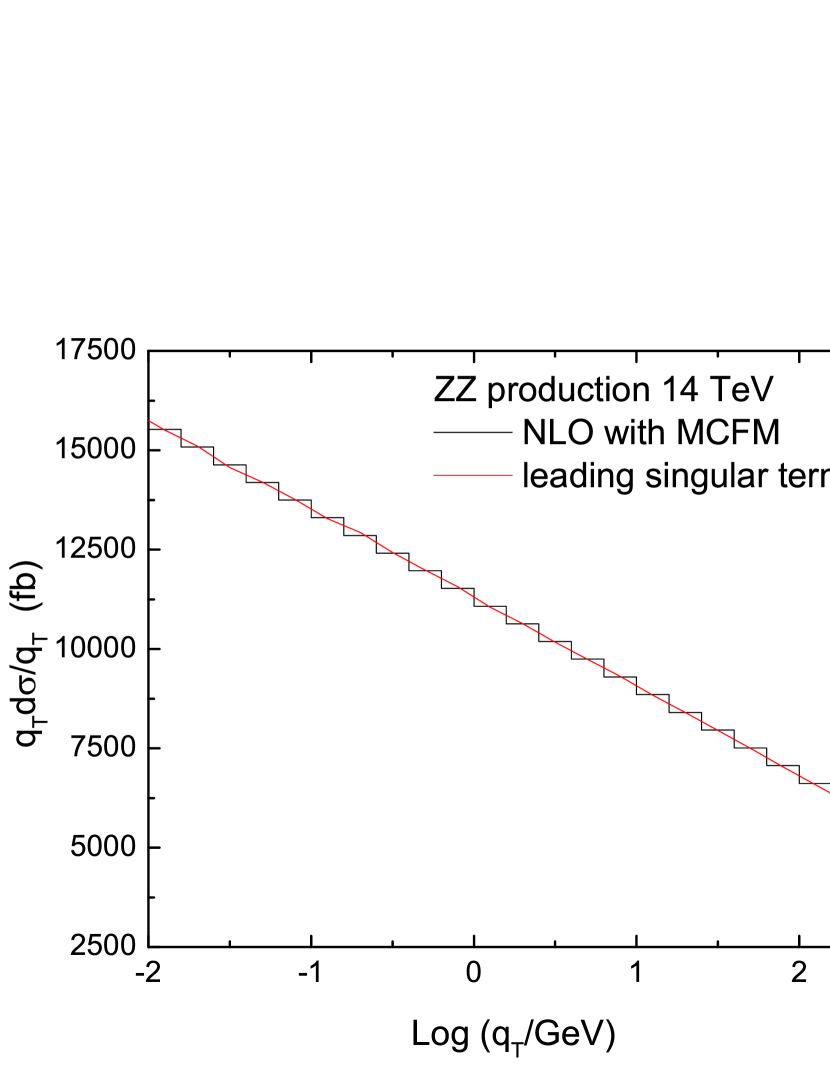
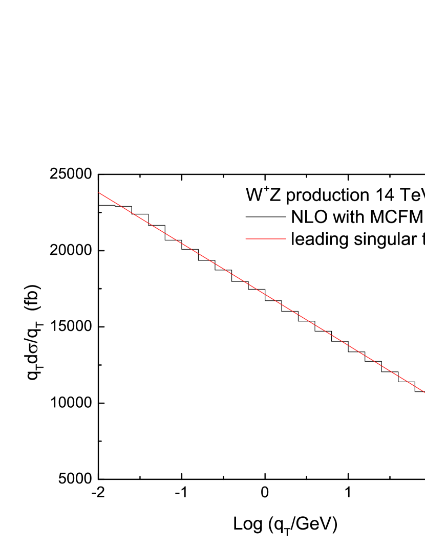
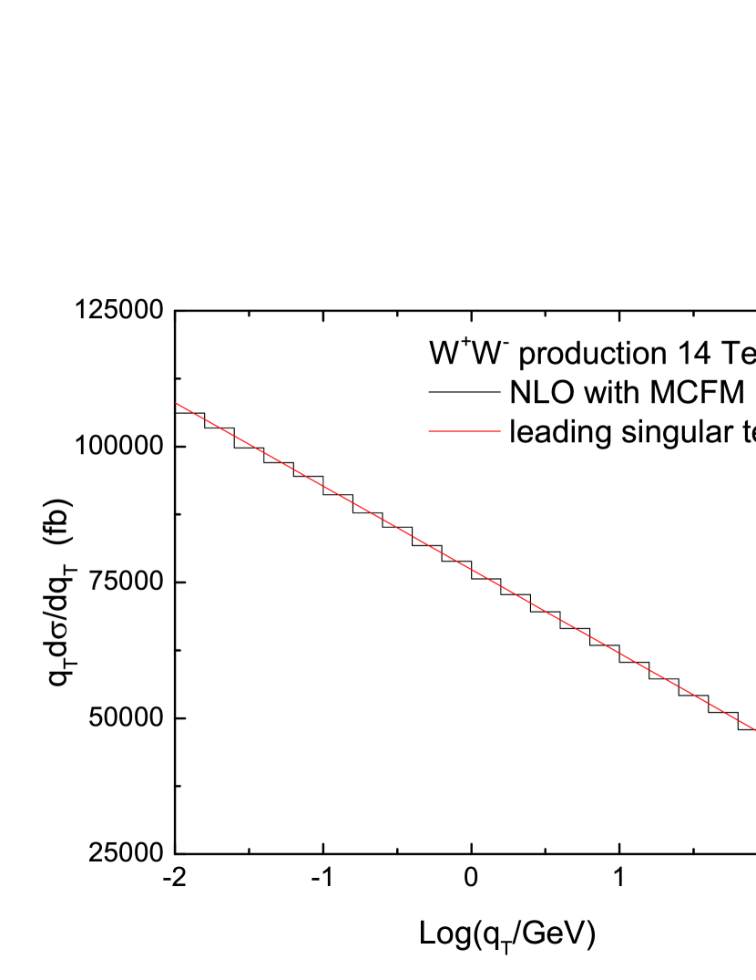
Figure 1: Comparison of the leading singular (red) and the exact NLO (black) distributions in the small $q_{T}$ region.

III.1 Fixed-order Results And Non-perturbative Effects

When resummation formula Eq. (16) is expanded to $\mathcal{O}(\alpha_{s})$ in the limit $q_{T}\rightarrow 0$, the leading singular predictions should agree with the exact NLO results Becher et al. (2012b). In Fig. 1, we compare the leading singular results and exact NLO results calculated by MCFM. It is shown that they are consistent with each other.

When discussing operator-product expansion of the transverse-position dependent PDFs $\mathcal{B}_{q/N}$, a hadronic form factor $f_{\rm hadr}(x_{T}\Lambda_{NP})$, parameterized in terms of a hadronic scale $\Lambda_{NP}$, is needed to be introduced in the region $q_{T}\sim\Lambda_{QCD}$ Becher et al. (2012b), and $\mathcal{B}_{q/N}$ can be expressed as

$$\mathcal{B}_{q/N}(z,x_{T}^{2},\mu_{f})=\mathcal{B}_{q/N}^{pert}(z,x_{T}^{2},\mu_{f})f_{\rm hadr}(x_{T}\Lambda_{NP}).$$ (20)

Here the form factor has the form

$$f_{\rm hadr}(x_{T}\Lambda_{NP})=\exp(-x_{T}^{2}\Lambda_{NP}^{2}).$$ (21)

In Fig. 2, we present the non-perturbative effects on the differential cross sections of gauge boson pair resummation at the LHC with $\sqrt{S}=14~{}\text{TeV}$. Obviously, Fig. 2 shows that the non-perturbative effects result in a tiny shift on the $q_{T}$ spectrum. We choose $\Lambda_{NP}=0.6$ GeV in the following numerical calculations.

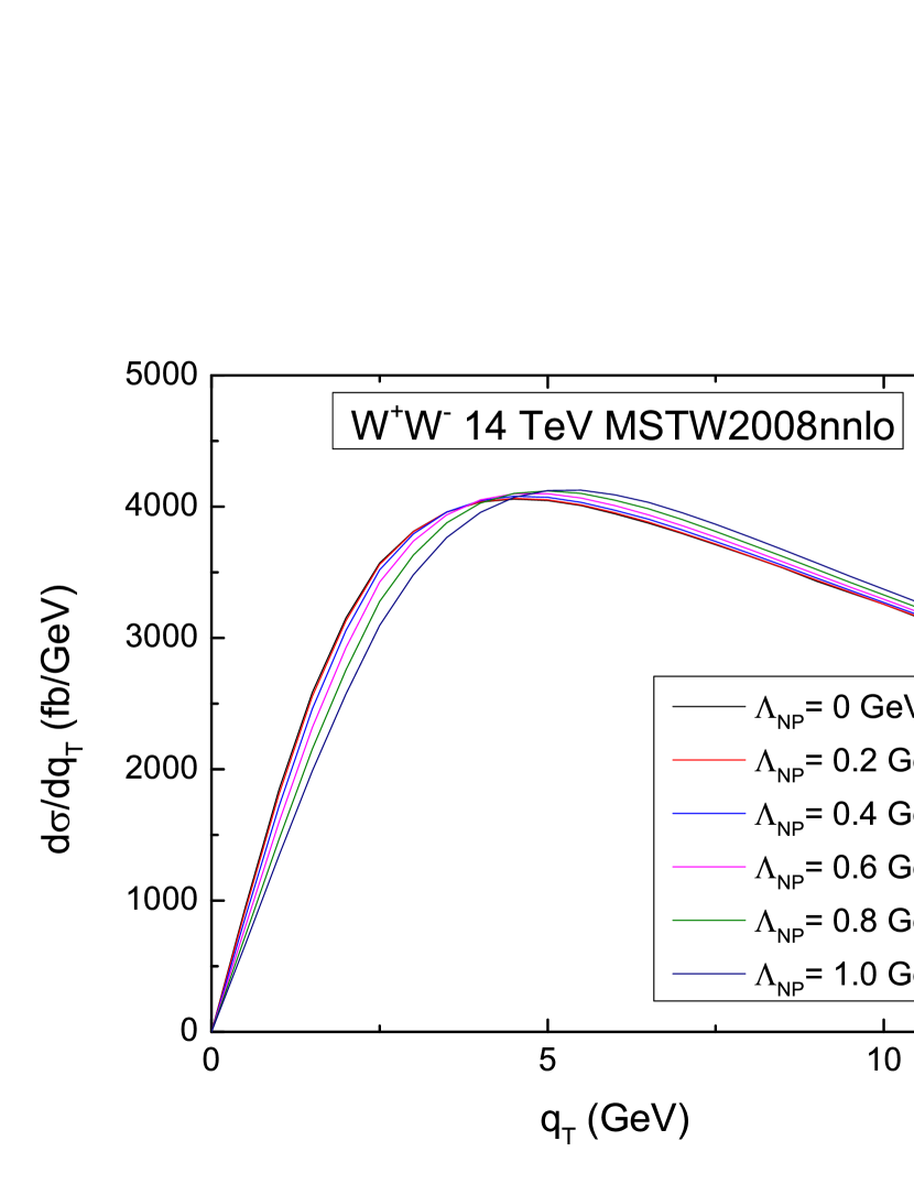
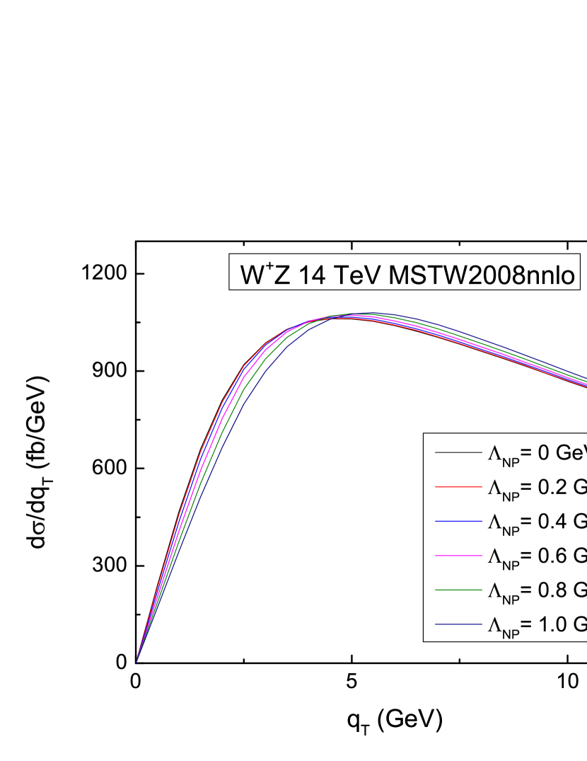
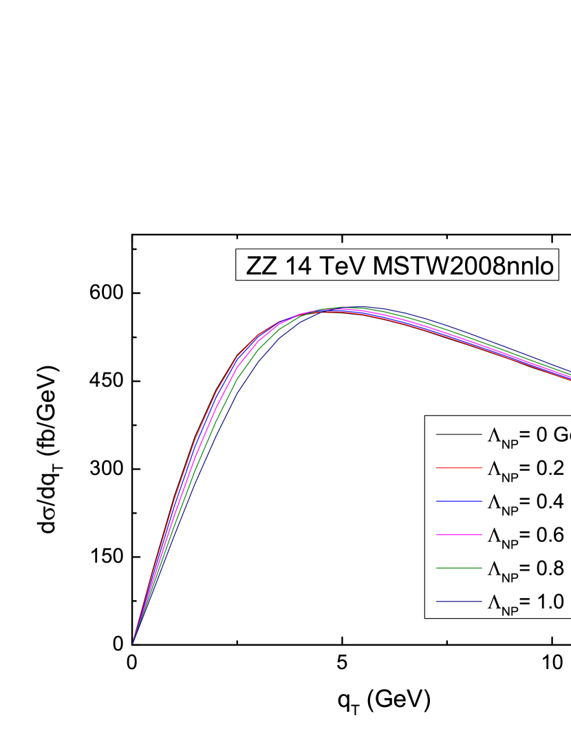
Figure 2: The non-perturbative effects on the differential cross sections of gauge boson pair production with $\sqrt{S}=14~{}\text{TeV}$, respectively.

III.2 Resummation Results

Fig. 3 shows the resummed $q_{T}$ distributions for $W^{+}W^{-},~{}ZZ$, and $W^{+}Z$ productions at next-to-leading logarithmic (NLL) and NNLL + NLO accuracy at the LHC with $\sqrt{S}=8$ TeV and $\sqrt{S}=14$ TeV, respectively, which include the uncertainties of the theoretical predictions by varying the factorization scale $\mu_{f}$ by a factor of two around the default choice. In these three cases of the gauge boson pair productions, the peak heights of the $q_{T}$ spectrums for $\sqrt{S}=14~{}\text{TeV}$ are much larger than that for $\sqrt{S}=8~{}\text{TeV}$, and the peak positions have a shift of about 0.5 GeV, respectively. Besides it is shown that, compared with the NLL results, the NNLL + NLO predictions significantly reduce the scale uncertainties, which make the theoretical predictions more reliable. In Fig. 3 the K factors, defined as $\sigma_{\text{NNLL+NLO}}/\sigma_{\text{NLO}}$, are also shown. The fixed-order predictions is calculated by MCFM, and is invalid at small $q_{T}$ region. In these three cases, at $q_{T}=50~{}\text{GeV}$, the K factors are 1.7-1.8 for $\sqrt{S}=8~{}\text{TeV}$ and 1.5-1.6 for $\sqrt{S}=14~{}\text{TeV}$, respectively. And in the very large $q_{T}$ region resumed results agree with MCFM predictions. Note that, to our knowledge, the $q_{T}$ distribution of $W^{\pm}Z$ production at NNLL + NLO accuracy is not available in both SCET and CSS frames before.

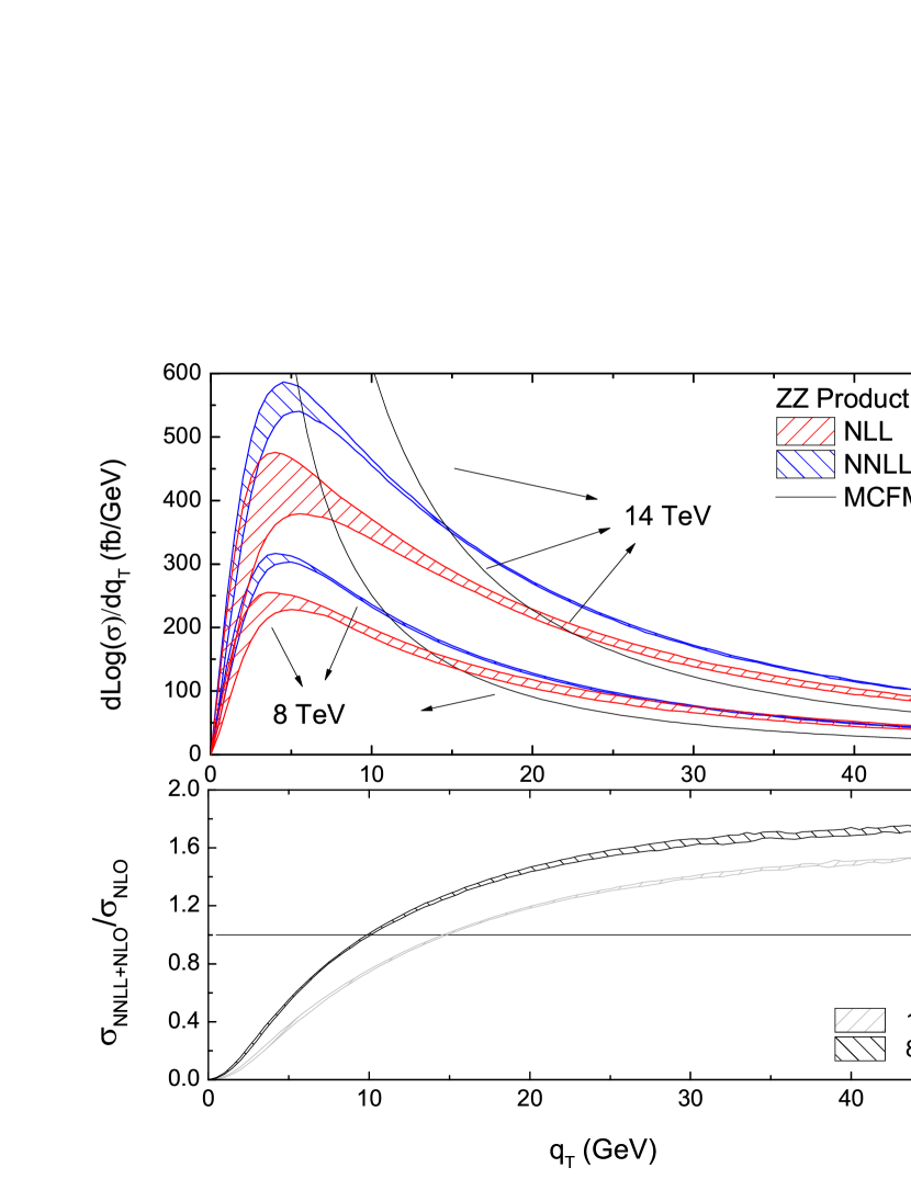
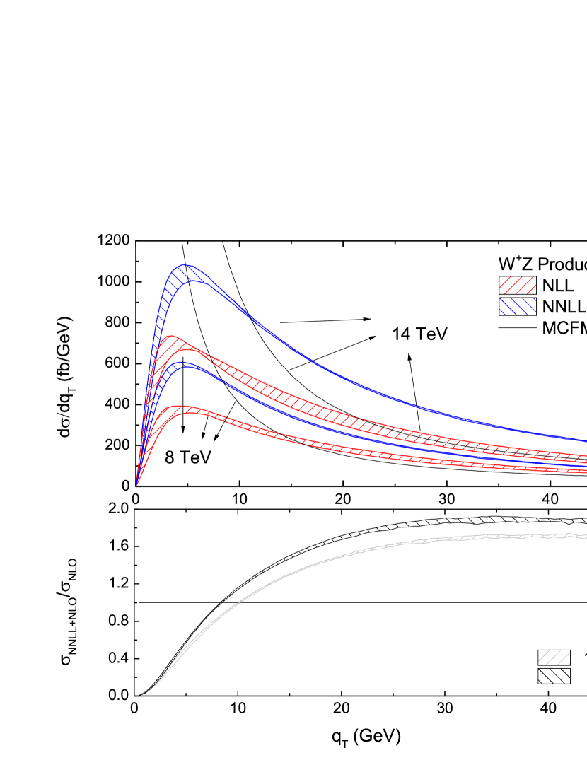
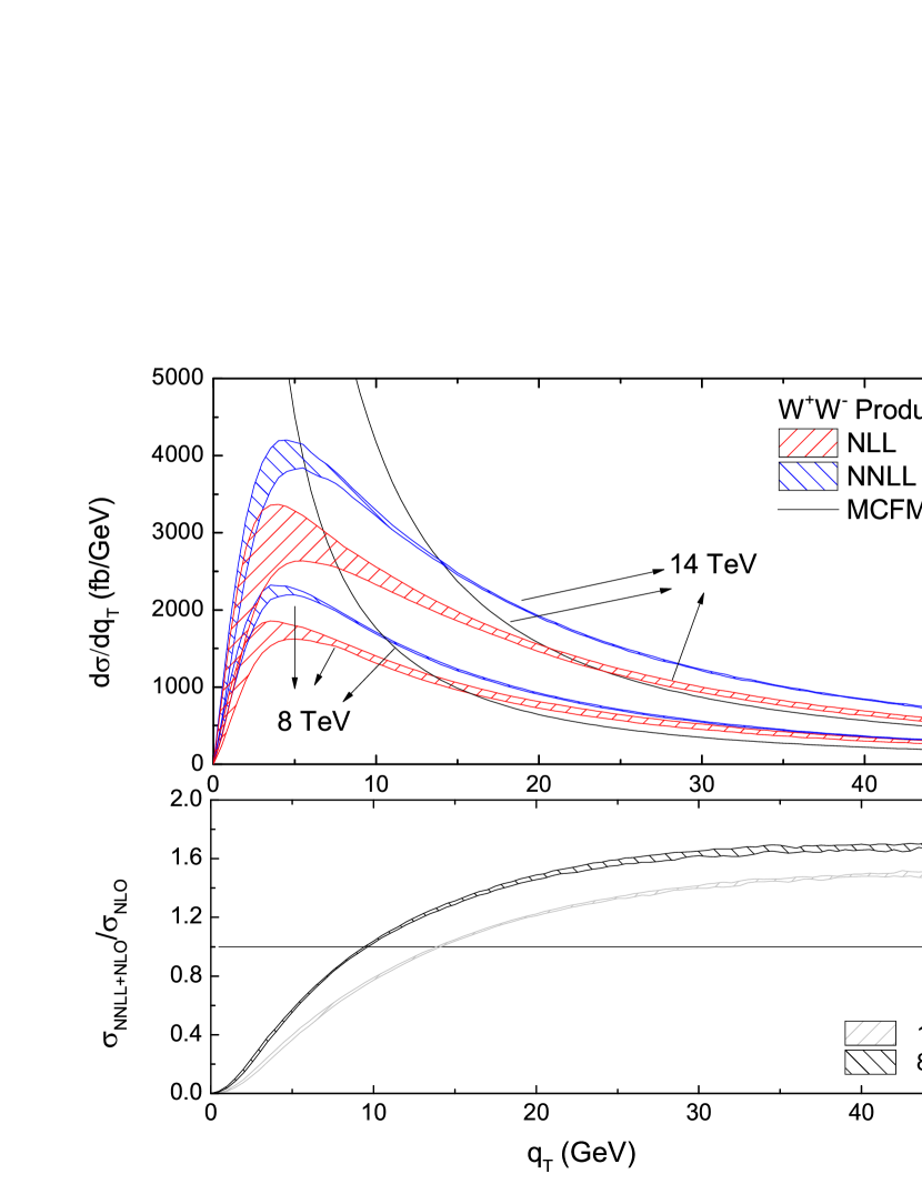
Figure 3: Up: the $q_{T}$ distributions with scale uncertainties for gauge boson pair productions at the LHC with $\sqrt{S}=8~{}\text{TeV}$ and $\sqrt{S}=14~{}\text{TeV}$. Down: NNLL + NLO results normalized to NLO.

In Fig. 4, we show the PDF uncertainties of the NNLL order transverse-momentum distributions of the gauge boson pair at $2\sigma$ deviation for $\sqrt{S}=14~{}\text{TeV}$. The PDF uncertainties are of order 5% at low $q_{T}$ region, and decrease to 2.5% at high $q_{T}$ region for all three cases, respectively. We also show the PDF uncertainties with CT10NNLO PDF sets in the same plots, and the PDF uncertainties are a little larger than the cases with MSTW2008NNLO PDF sets. The situations for $\sqrt{S}=8~{}\text{TeV}$ are almost the same, and we do not discuss them here.

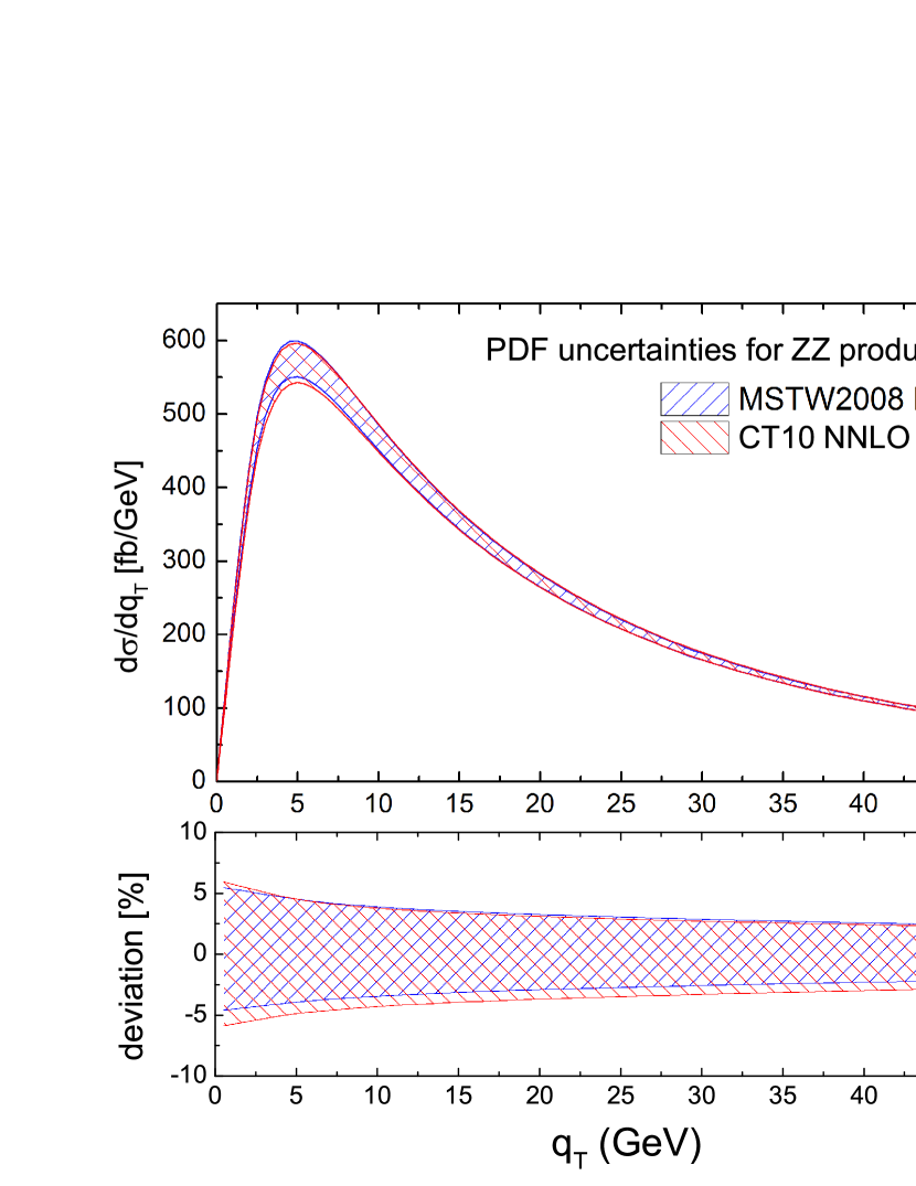
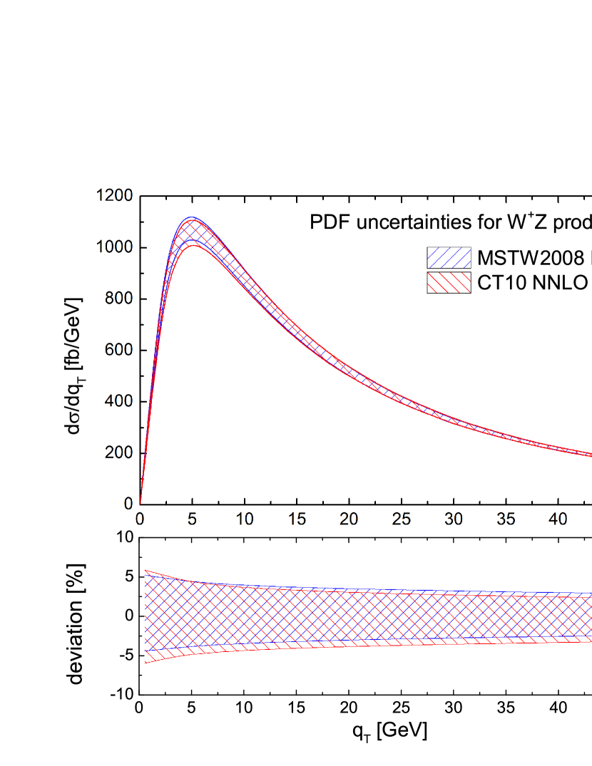
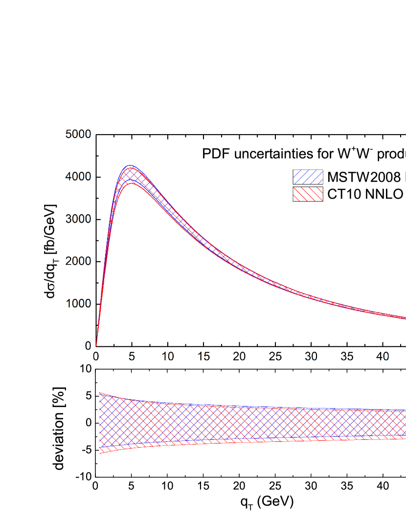
Figure 4: The PDF uncertainties of NNLL order resummed transverse-momentum for gauge boson pair production, where the bands represent 2$\sigma$ deviation.

In Fig. 5, we compare our NNLL + NLO results with previous studies Grazzini (2005); Frederix and Grazzini (2008) in CSS frame with MRST2002NLO PDF set for $\sqrt{S}=14~{}\text{TeV}$. The peak positions of the transverse-momentum spectrum for $W^{+}W^{-}$ and $ZZ$ productions in our results and those in CSS results are both at about 5 GeV. However, as shown in Fig. 5, in the small $q_{T}$ region, the peaks height in our results are a little lower than those in CSS frame. Probably, this is due to the fact that the choices of scales in two scheme are different. In CSS frame, the renormalization and the factorization scale are set to 2$m_{W/Z}$, and resummation scale is the invariant mass of the gauge boson pair. However in SCET frame there are only factorization scale and hard scale. The factorization scale is chosen as $q^{*}+q_{T}$, as described in Sec. II, while the hard scale is taken as the invariant mass of the gauge boson pair.

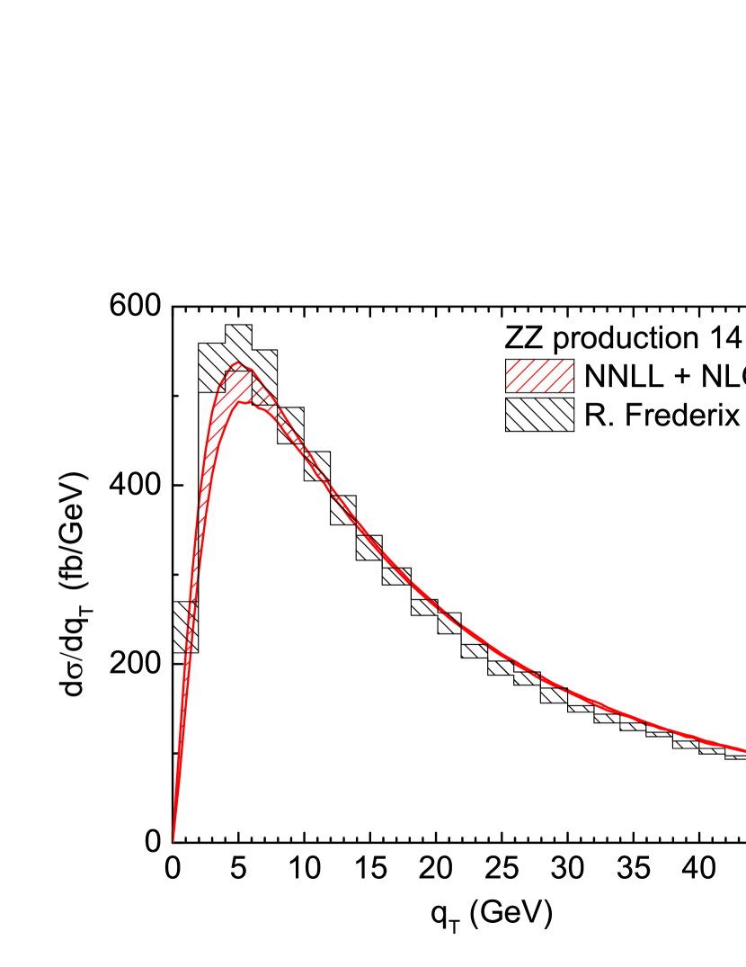
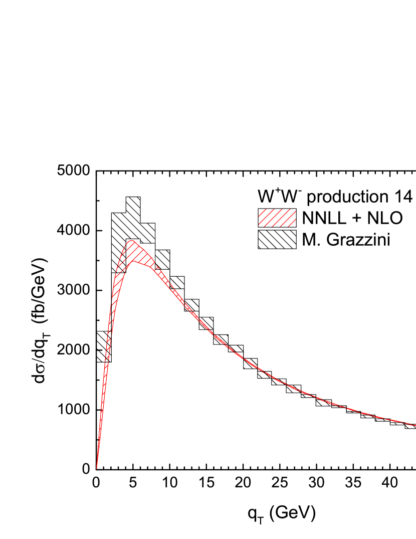
Figure 5: Comparison of NNLL + NLO resummed $q_{T}$ distribution for $W^{+}W^{-}$ and $ZZ$ distributions in the SCET and CSS frame at $\sqrt{S}=14~{}\text{TeV}$ with MRST2002NLO PDF set.

In Fig. 6, we compare the resummed results for the normalized differential cross section with the experimental data measured by the CMS collaboration CMS (2013) for $ZZ$ production at the LHC with $\sqrt{S}=8$ TeV. Obviously, our NNLL + NLO predictions are consistent with the experimental data within theoretical and experimental uncertainties.

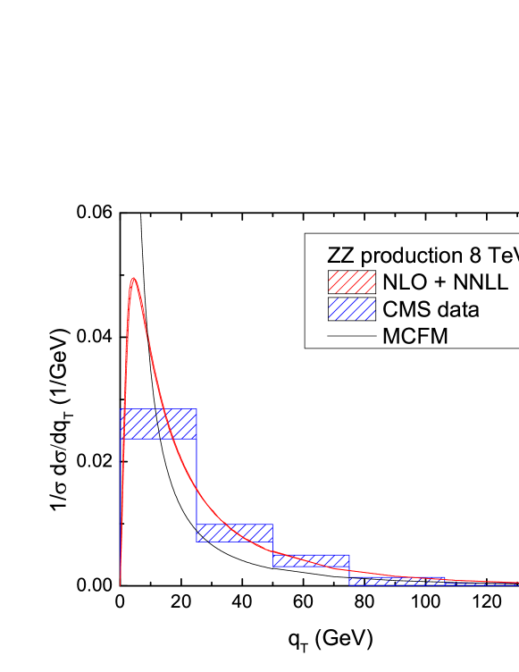
Figure 6: Comparison of normalized $q_{T}$ distribution for $ZZ$ productions between CMS experimental data and resummation prediction at the LHC with $\sqrt{S}=8$ TeV.

IV Conclusion

We have studied the transverse-momentum resummation for $W^{+}W^{-}$, $ZZ$, and $W^{\pm}Z$ pair productions at the NNLL + NLO accuracy with SCET at the LHC. Especially, this is the first calculation of $W^{\pm}Z$ transverse-momentum resummation at the NNLL + NLO accuracy. The non-perturbative effects are also included in our calculations. In these three cases of the gauge boson pair productions, our results show that the peak positions are all around $5~{}\text{GeV}$ for $\sqrt{S}=8~{}\text{TeV}$ and $\sqrt{S}=14~{}\text{TeV}$, respectively, which agree quite well with previous results for $W^{+}W^{-}$ and $ZZ$ productions, and the PDF uncertainties are less than 5% at the $2\sigma$ level for the peak region. We also find that our results agree well with experimental data reported by the CMS collaborations for the $ZZ$ productions at $\sqrt{S}=8~{}\text{TeV}$ within theoretical and experimental uncertainties.

V Acknowledgements

This work was supported by the National Natural Science Foundation of China, under Grants No. 11021092 and No. 11135003.

Appendix A Results of hard function

Here, we show the detail results of $\mathcal{H}_{V_{l}V_{m}}(M,\mu_{h})$ of the gauge boson pair production. We define

$$\mathcal{H}_{V_{l}V_{m}}(M,\mu_{h})=\frac{1}{2s}\int H_{V_{l}V_{m}}(s,t,u,\mu_{h})\frac{d^{3}p_{3}}{(2\pi)^{3}2E_{3}}\frac{d^{3}p_{4}}{(2\pi)^{3}2E_{4}}(2\pi)^{4}\delta^{4}(q-p_{3}-p_{4}),$$ (22)

and expand $H_{V_{l}V_{m}}$ as

$$H_{V_{l}V_{m}}=H_{V_{l}V_{m}}^{(0)}+\frac{\alpha_{s}}{2\pi}H_{V_{l}V_{m}}^{(1)}.$$ (23)

The leading order coefficient is

$$H_{V_{l}V_{m}}^{(0)}=\overline{|\mathcal{M}^{B}_{V_{l}V_{m}}|^{2}},$$ (24)

where $\overline{|\mathcal{M}^{B}_{V_{l}V_{m}}|^{2}}$ is the color-averaged and spin-averaged tree-level matrix element squared. $H_{{V_{l}V_{m}}}^{(1)}$ can be divided into two parts

$$H_{V_{l}V_{m}}^{(1)}=\frac{\alpha_{s}}{2\pi}\left(H_{V_{l}V_{m},\text{reg}}^{(1)}+H_{\mu}^{(1)}\right).$$ (25)

where $H_{\mu}^{(1)}$ has the same form for three cases:

$$H_{\mu}^{(1)} = C_{F}H_{V_{l}V_{m}}^{(0)}\left(-\ln^{2}\frac{M^{2}}{\mu_{h}^{2}}+3\ln\frac{M^{2}}{\mu_{h}^{2}}-\frac{\pi^{2}}{6}\right).$$ (26)

For simplicity, we define that all scalar one-loop integrals should be understood as retaining the finite part, and

$$\text{C}_{0}^{s} = \text{C}_{0}\left(0,0,s,0,0,0\right),$$

$$\text{C}_{0}^{V_{1},V_{2}} = \text{C}_{0}\left(m_{V_{1}}^{2},s,m_{V_{2}}^{2},0,0,0\right),$$

$$\text{C}^{V,t}_{0} = \text{C}_{0}\left(0,m_{V}^{2},t,0,0,0\right),$$

$$\text{D}_{0}^{V_{1},V_{2}} = \text{D}_{0}\left(0,0,m_{V_{1}}^{2},m_{V_{2}}^{2},s,t,0,0,0,0\right).$$ (27)

A.1 $ZZ$ production

The leading order (LO) coefficient is Mele et al. (1991)

$$H_{ZZ}^{(0)} = \frac{1}{N_{c}}((g_{i,Z}^{L})^{4}+(g_{i,Z}^{R})^{4})\times$$ (28)

$$\left(\frac{-\left(m_{Z}\right){}^{4}\left(t^{2}-8tu+u^{2}\right)-4tu\left(m_{Z}\right){}^{2}(t+u)+tu\left(t^{2}+u^{2}\right)}{t^{2}u^{2}}\right).$$

where $g_{i,Z}^{L,R},~{}i=u,d$ is the couplings between the $Z$ boson and quarks

$$g_{u,Z}^{L} = \frac{e}{\sin\theta_{W}\cos\theta_{W}}\left(\frac{1}{2}-\frac{2\sin^{2}\theta_{W}}{3}\right),$$

$$g_{d,Z}^{L} = \frac{e}{\sin\theta_{W}\cos\theta_{W}}\left(-\frac{1}{2}+\frac{\sin^{2}\theta_{W}}{3}\right),$$

$$g_{u,Z}^{R} = -\frac{2}{3}\tan\theta_{W},$$

$$g_{d,Z}^{R} = -\frac{1}{3}\tan\theta_{W},$$ (29)

where $\theta_{W}$ is the Weinberg angle. The functions at the $\mathcal{O}(\alpha_{s})$ are Mele et al. (1991),

$$\frac{\alpha_{s}}{2\pi}H_{ZZ,\text{reg}}^{(1)} = \frac{1}{12}\frac{\alpha_{s}}{2\pi}C_{F}((g_{i,Z}^{L})^{4}+(g_{i,Z}^{R})^{4})$$ (30)

$$\bigg{(}\text{A1}(t,u)+\text{A2}(t,u)\ln\left(-\frac{m_{Z}^{2}}{t}\right)+\text{A3}(t,u)\ln\left(-\frac{m_{Z}^{2}}{s}\right)+\text{A4}(t,u)\text{D}_{0}^{Z,Z}$$

$$+\text{A5}(t,u)\text{C}^{Z,t}_{0}+\text{A6}(t,u)\text{C}_{0}^{Z,Z}+\text{A7}(t,u)\text{C}_{0}^{s}+(t\Leftrightarrow u)\bigg{)},$$

where

$$A1(t,u) = \frac{2\left(m_{Z}^{2}+t\right)^{2}}{stu\left(1-\frac{4m_{Z}^{2}}{s}\right)}+\frac{4s}{u\left(t-m_{Z}^{2}\right)}$$

$$-\frac{-36m_{Z}^{6}+18m_{Z}^{4}s+t^{2}\left(28s-68m_{Z}^{2}\right)+t\left(88m_{Z}^{4}-36m_{Z}^{2}s+18s^{2}\right)+16t^{3}}{st^{2}u},$$

$$A2(t,u)=-\frac{6\left(m_{Z}^{4}+s^{2}\right)}{stu}-\frac{4m_{Z}^{2}s}{u\left(t-m_{Z}^{2}\right)^{2}}+\frac{12s}{u\left(t-m_{Z}^{2}\right)}+\frac{6m_{Z}^{4}\left(2m_{Z}^{2}-s\right)}{st^{2}u}+\frac{2(4s+t)}{su},$$

$$A3(t,u) = -\frac{-12m_{Z}^{6}+t\left(25m_{Z}^{4}+6s^{2}\right)+6m_{Z}^{4}s+t^{2}\left(8s-18m_{Z}^{2}\right)+5t^{3}}{st^{2}u}$$ (33)

$$\frac{-25m_{Z}^{4}-26m_{Z}^{2}t+3t^{2}}{stu\left(1-\frac{4m_{Z}^{2}}{s}\right)}-\frac{12m_{Z}^{2}\left(m_{Z}^{2}+t\right)^{2}}{s^{2}tu\left(1-\frac{4m_{Z}^{2}}{s}\right)^{2}},$$

$$A4(t,u) = \frac{-12m_{Z}^{4}+8m_{Z}^{2}t-2s^{2}-2t^{2}}{u}+\frac{4m_{Z}^{4}\left(2m_{Z}^{2}-s\right)}{tu},$$ (34)

$$A5(t,u) = \frac{8m_{Z}^{6}\left(2m_{Z}^{2}-s\right)}{st^{2}u}+\frac{4\left(10m_{Z}^{4}-5m_{Z}^{2}t+s^{2}+t^{2}\right)}{su}$$ (35)

$$+\frac{4m_{Z}^{2}\left(-10m_{Z}^{4}+2m_{Z}^{2}s-s^{2}\right)}{stu},$$

$$A6(t,u) = \frac{-3m_{Z}^{6}+12m_{Z}^{4}s-4m_{Z}^{2}s^{2}+t^{2}\left(2s-3m_{Z}^{2}\right)+t\left(6m_{Z}^{4}-8m_{Z}^{2}s\right)+2s^{3}}{stu}$$ (36)

$$+\frac{12m_{Z}^{4}\left(m_{Z}^{2}+t\right)^{2}}{s^{2}tu\left(1-\frac{4m_{Z}^{2}}{s}\right)^{2}}-\frac{-27m_{Z}^{6}-30m_{Z}^{4}t+m_{Z}^{2}t^{2}}{stu\left(1-\frac{4m_{Z}^{2}}{s}\right)},$$

$$A7(t,u) = \frac{4}{3}\left(\frac{\left(s-2m_{Z}^{2}\right)^{2}}{stu}+\frac{-4m_{Z}^{2}+4s+t}{su}\right).$$ (37)

A.2 $W^{\pm}Z$ production

The LO results can be expressed as Frixione et al. (1992):

$$H_{WZ}^{(0)} = \frac{1}{6}\left(\frac{1}{2\sqrt{2}\sin\theta_{W}}\right)^{2}\Bigg{(}(g_{d,Z}^{L})^{2}I_{dd}^{(0)}(s,t,u)+2g_{d,Z}^{L}g_{u,Z}^{L}I_{ud}^{(0)}(s,t,u)+(g_{u,Z}^{L})^{2}I_{dd}^{(0)}(s,u,t)$$ (38)

$$+2g_{W,Z}g_{d,Z}(F_{d}^{(0)}(s,t,u)-F_{d}^{(0)}(s,u,t))+g_{W,Z}^{2}J^{(0)}(s,t,u)\Bigg{)},$$

where

$$g_{W,Z} = \frac{-e}{s-m_{W}^{2}}\frac{\cos\theta_{W}}{\sin\theta_{W}},$$ (39)

and

$$I_{dd}^{(0)}(s,t,u) = 8\left(\frac{s\left(m_{W}^{2}+m_{Z}^{2}\right)}{2m_{W}^{2}m_{Z}^{2}}+\frac{1}{4}\left(\frac{tu}{m_{W}^{2}m_{Z}^{2}}-1\right)\right)+8\left(\frac{u}{t}-\frac{m_{W}^{2}m_{Z}^{2}}{t^{2}}\right),$$ (40)

$$I_{ud}^{(0)}(s,t,u) = \frac{8s\left(m_{W}^{2}+m_{Z}^{2}\right)}{tu}-8\left(\frac{s\left(m_{W}^{2}+m_{Z}^{2}\right)}{2m_{W}^{2}m_{Z}^{2}}+\frac{1}{4}\left(\frac{tu}{m_{W}^{2}m_{Z}^{2}}-1\right)\right),$$ (41)

$$F_{d}^{(0)}(s,t,u) = -8s\Bigg{(}\frac{1}{4}\left(-\frac{4m_{W}^{2}m_{Z}^{2}}{st}-\frac{m_{W}^{2}+m_{Z}^{2}}{s}+1\right)\left(\frac{tu}{m_{W}^{2}m_{Z}^{2}}-1\right)$$ (42)

$$+\frac{\left(m_{W}^{2}+m_{Z}^{2}\right)\left(\frac{2m_{W}^{2}m_{Z}^{2}}{t}-m_{W}^{2}-m_{Z}^{2}+s\right)}{2m_{W}^{2}m_{Z}^{2}}\Bigg{)},$$

$$J^{(0)}(s,t,u) = 8s^{2}\left(\frac{8m_{W}^{2}m_{Z}^{2}+\left(m_{W}^{2}+m_{Z}^{2}\right)^{2}}{4s^{2}}-\frac{m_{W}^{2}+m_{Z}^{2}}{2s}+\frac{1}{4}\right)\left(\frac{tu}{m_{W}^{2}m_{Z}^{2}}-1\right)$$ (43)

$$+\frac{8s^{2}\left(m_{W}^{2}+m_{Z}^{2}\right)\left(\frac{\left(m_{W}^{2}-m_{Z}^{2}\right)^{2}}{2s}-m_{W}^{2}-m_{Z}^{2}+\frac{s}{2}\right)}{m_{W}^{2}m_{Z}^{2}}.$$

When considering virtual corrections, as in the tree level case, we have Frixione et al. (1992)

$$\frac{\alpha_{s}}{2\pi}H_{WZ,\text{reg}}^{(1)} = \frac{1}{6}\frac{\alpha_{s}}{2\pi}C_{F}\left(\frac{1}{2\sqrt{2}\sin\theta_{W}}\right)^{2}$$ (44)

$$\Bigg{(}(g_{d,Z}^{L})^{2}I_{dd}^{(1)}(s,t,u)+g_{d,Z}^{L}g_{u,Z}^{L}I_{ud}^{(1)}(s,t,u)+(g_{u,Z}^{L})^{2}I_{dd}^{(1)}(s,u,t)$$

$$+g_{W,Z}g_{d,Z}(F_{d}^{(1)}(s,t,u)-F_{d}^{(1)}(s,u,t))+g_{W,Z}^{2}J^{(1)}(s,t,u)\Bigg{)},$$

where

$$I_{dd}^{(1)} = \frac{2\left(22t^{2}+t(19s-18\Sigma)+18m_{W}^{2}m_{Z}^{2}\right)}{t^{2}}-\frac{8(ut+2s\Sigma)}{m_{W}^{2}m_{Z}^{2}}-\frac{2(t-u)^{2}}{ts\beta^{2}}$$ (45)

$$+\Bigg{(}\frac{2\left(8t^{2}+4t(s-3\Sigma)+4\Sigma^{2}-5s\Sigma+s^{2}\right)}{ts\beta^{2}}+\frac{4\left(t(3u+s)-3m_{W}^{2}m_{Z}^{2}\right)}{t^{2}}$$

$$+\frac{6(t+u)(t-u)^{2}}{ts^{2}\beta^{4}}\Bigg{)}\ln\left(-\frac{t}{s}\right)$$

$$+\Bigg{(}\frac{8t^{2}(-2s+\Delta)+8t\left(-s^{2}+3s\Sigma-2\Delta\Sigma\right)-2(s-\Sigma)\left(s^{2}-4s\Sigma+3\Delta\Sigma\right)}{ts^{2}\beta^{2}}$$

$$+\frac{16s\left(t-m_{Z}^{2}\right)}{t(u+s)-m_{W}^{2}m_{Z}^{2}}-\frac{6(s-\Delta)(t+u)(t-u)^{2}}{ts^{3}\beta^{4}}$$

$$+\frac{2\left(4t^{2}+t\left(10s-3m_{Z}^{2}-9m_{W}^{2}\right)+12m_{W}^{2}m_{Z}^{2}\right)}{t^{2}}\Bigg{)}\ln\left(-\frac{t}{m_{W}^{2}}\right)$$

$$+\bigg{(}-\frac{4t^{2}(2\Sigma-3s)-4t(s-\Sigma)(2s-3\Sigma)-2(s-2\Sigma)(s-\Sigma)^{2}}{ts\beta^{2}}$$

$$+\frac{4\Sigma t-3s^{2}+4s\Sigma-4\left(m_{W}^{4}+m_{Z}^{4}\right)}{t}-\frac{3\left(t^{2}-u^{2}\right)^{2}}{ts^{2}\beta^{4}}\bigg{)}\text{C}_{0}^{W,Z}$$

$$+\left(\frac{4(ut+2s\Sigma)}{3m_{W}^{2}m_{Z}^{2}}-\frac{4(t-2u)}{3t}\right)\text{C}_{0}^{s}-\frac{4s\left(tu-2m_{W}^{2}m_{Z}^{2}\right)\text{D}_{0}^{W,Z}}{t}$$

$$+\frac{\left(8\left(t-m_{W}^{2}\right)\left(ut-2m_{W}^{2}m_{Z}^{2}\right)\right)\text{C}^{W,t}_{0}}{t^{2}}+(m_{W}\Leftrightarrow m_{Z}),$$

$$I_{ud}^{(1)} = \frac{4s^{2}(2t-\Sigma)}{u\left(m_{W}^{2}m_{Z}^{2}-t(s+u)\right)}+\frac{8(2s\Sigma+tu)}{m_{W}^{2}m_{Z}^{2}}+\frac{2\left(-18s\Sigma+t(9s-4\Sigma)+4t^{2}\right)}{tu}$$ (46)

$$+\Bigg{(}\frac{2\left(-(s-\Sigma)(3s+4\Sigma)-4t(s+3\Sigma)+8t^{2}\right)}{\beta^{2}su}$$

$$+\frac{6(t+u)(t-u)^{2}}{\beta^{4}s^{2}u}-\frac{12s(t-\Sigma)}{tu}\Bigg{)}\ln\left(-\frac{t}{s}\right)$$

$$\Bigg{(}\frac{2}{us^{2}\beta^{2}}\Big{(}4t^{2}(-2s+\Delta)+4t(s^{2}+s(m_{Z}^{2}+5m_{W}^{2})-2\Delta\Sigma)$$

$$+(s-\Sigma)(3\ s^{2}+8sm_{W}^{2}-3\Delta\Sigma)\Big{)}-\frac{8s^{2}t\left(t-m_{Z}^{2}\right)(2t-\Sigma)}{u\left(m_{W}^{2}m_{Z}^{2}-t(s+u)\right)^{2}}$$

$$+\frac{2t\left(2m_{W}^{2}+m_{Z}^{2}+18s\right)-24s\Sigma}{tu}+\frac{6(s-\Delta)(s-\Sigma)(t-u)^{2}}{\beta^{4}s^{3}u}$$

$$-\frac{8s\left(-t\left(2m_{W}^{2}+4m_{Z}^{2}+3s\right)+2m_{Z}^{2}(s+\Sigma)+2t^{2}\right)}{u\left(m_{W}^{2}m_{Z}^{2}-t(s+u)\right)}\Bigg{)}\ln\left(-\frac{t}{m_{W}^{2}}\right)$$

$$\Bigg{(}-\frac{2\left((s-\Sigma)^{2}(s+2\Sigma)+2t^{2}(2\Sigma-3s)+6\Sigma t(s-\Sigma)\right)}{\beta^{2}su}$$

$$+\frac{3s(-s-4\Sigma+4t)}{u}-\frac{2(t-u)^{2}}{\beta^{2}su}-\frac{3(s-\Sigma)^{2}(t-u)^{2}}{\beta^{4}s^{2}u}\Bigg{)}\text{C}_{0}^{W,Z}+\frac{8s^{2}(t-\Sigma)}{u}\text{D}_{0}^{W,Z}$$

$$+\left(\frac{4(4s+u)}{3u}-\frac{4(2s\Sigma+tu)}{3m_{W}^{2}m_{Z}^{2}}\right)\text{C}_{0}^{s}+\frac{16s\left(t-m_{W}^{2}\right)(t-\Sigma)}{tu}\text{C}^{W,t}_{0}$$

$$+(t\Leftrightarrow u)+(m_{W}\Leftrightarrow m_{Z})+(t\Leftrightarrow u,m_{W}\Leftrightarrow m_{Z}),$$

$$F_{d}^{(1)} = \frac{4\left(17\left(m_{W}^{2}m_{Z}^{2}+s\Sigma\right)+t(11s-13\Sigma)+17t^{2}\right)}{t}$$ (47)

$$+\frac{16(s-\Sigma)(2s\Sigma+tu)}{m_{W}^{2}m_{Z}^{2}}+\frac{4s^{2}(2t-\Sigma)}{t(s+u)-m_{W}^{2}m_{Z}^{2}}$$

$$+\left(\frac{8(t-u)}{\beta^{2}}-\frac{4\left(3\left(m_{W}^{2}m_{Z}^{2}+s\Sigma\right)-t(s+3\Sigma)+3t^{2}\right)}{t^{2}}\right)\ln\left(-\frac{t}{s}\right)$$

$$\Bigg{(}\frac{8\left(3\left(m_{W}^{2}m_{Z}^{2}+s\Sigma\right)-t\left(3m_{W}^{2}+m_{Z}^{2}+2s\right)+t^{2}\right)}{t}+\frac{8s\left(t(3s+2\Sigma)-2m_{Z}^{2}(s+\Sigma)\right)}{t(s+u)-m_{W}^{2}m_{Z}^{2}}$$

$$\frac{8s^{2}t\left(t-m_{Z}^{2}\right)(2t-\Sigma)}{\left(t(s+u)-m_{W}^{2}m_{Z}^{2}\right)^{2}}-\frac{8(s-\Delta)(t-u)}{\beta^{2}s}\Bigg{)}\ln\left(-\frac{t}{m_{W}^{2}}\right)$$

$$4\left(-m_{W}^{4}-m_{Z}^{4}+4s\Sigma\right)+4t(\Sigma-3s)+\frac{4(s-\Sigma)(t-u)}{\beta^{2}}\text{C}_{0}^{W,Z}$$

$$-\frac{8\left(2\left(m_{W}^{2}m_{Z}^{2}+s\Sigma\right)+2t(2s-\Sigma)+3t^{2}\right)}{3t}+\frac{8(s-\Sigma)(2s\Sigma+tu)}{3m_{W}^{2}m_{Z}^{2}}\text{C}_{0}^{s}$$

$$4\left(2s\left(m_{W}^{2}m_{Z}^{2}+s\Sigma\right)+st^{2}-st(s+\Sigma)\right)\text{D}_{0}^{W,Z}$$

$$-\frac{8\left(t-m_{W}^{2}\right)\left(2\left(m_{W}^{2}m_{Z}^{2}+s\Sigma\right)-t(s+\Sigma)+t^{2}\right)}{t}\text{C}^{W,t}_{0}+(m_{W}\Leftrightarrow m_{Z}),$$

$$J^{(1)} = \left(16-\frac{8\pi^{2}}{3}\right)\big{(}m_{W}^{4}-\frac{(s-\Sigma)^{2}(2s\Sigma+tu)}{m_{W}^{2}m_{Z}^{2}}$$ (48)

$$+10m_{W}^{2}m_{Z}^{2}+m_{Z}^{4}+s^{2}+6s\Sigma+8t(s-\Sigma)+8t^{2}\big{)},$$

with

$$\Sigma = m_{Z}^{2}+m_{W}^{2},$$

$$\Delta = m_{Z}^{2}-m_{W}^{2},$$

$$\beta = \sqrt{1-\frac{(m_{W}+m_{Z})^{2}}{s}}\sqrt{1-\frac{(m_{W}-m_{Z})^{2}}{s}}.$$ (49)

A.3 $W^{+}W^{-}$ production

The LO results are Frixione (1993)

$$H_{WW}^{(0)}=\frac{1}{12}\left(c_{q}^{tt}F_{q}^{0}(s,t)+c_{q}^{ss}K_{q}^{0}(s,t)-c_{q}^{ts}J_{q}^{0}(s,t)\right).$$ (50)

The coefficients are

$$c_{q}^{tt} = {\pi^{2}\alpha^{2}\over\sin^{2}\theta_{W}},$$

$$c_{q}^{ts}(s) = {4\pi^{2}\alpha^{2}\over\sin^{2}\theta_{W}}{1\over s}\biggl{(}Q_{q}+{s\over s-m_{Z}^{2}}{1\over\sin^{2}\theta_{W}}(T_{3,q}-Q_{q}\sin^{2}\theta_{W})\biggr{)},$$

$$c_{q}^{ss}(s) = {16\pi^{2}\alpha^{2}\over s^{2}}\biggl{\{}\biggl{(}Q_{q}+{1\over 2\sin^{2}\theta_{W}}(T_{3,q}-2Q_{q}\sin^{2}\theta_{W}){s\over s-m_{Z}^{2}}\biggr{)}^{2}$$ (51)

$$+\biggl{(}{T_{3,q}\over 2\sin^{2}\theta_{W}}{s\over s-m_{Z}^{2}}\biggr{)}^{2}\biggr{\}},$$

with $T_{3,q}=\pm{1\over 2}$. The functions occurring in the lowest order amplitudes are,

$$F_{u}^{0}(s,t) = F_{d}^{0}(s,u)$$

$$= 16\biggl{(}{ut\over m_{W}^{4}}-1\biggr{)}\biggl{(}{1\over 4}+{m_{W}^{4}\over t^{2}}\biggr{)}+16{s\over m_{W}^{2}},$$

$$J_{u}^{0}(s,t) = -J_{d}^{0}(s,u)$$

$$= 16\biggl{(}{ut\over m_{W}^{4}}-1\biggr{)}\biggl{(}{s\over 4}-{m_{W}^{2}\over 2}-{m_{W}^{4}\over t}\biggr{)}+16s\biggl{(}{s\over m_{W}^{2}}-2+{2m_{W}^{2}\over t}\biggr{)},$$

$$K_{u}^{0}(s,t) = K_{d}^{0}(s,u)$$ (52)

$$= 8\biggl{(}{ut\over m_{W}^{4}}-1\biggr{)}\biggl{(}{s^{2}\over 4}-sm_{W}^{2}+3m_{W}^{4}\biggr{)}+8s^{2}\biggl{(}{s\over m_{W}^{2}}-4\biggr{)}\,.$$

The functions at the $\mathcal{O}(\alpha_{s})$ are Frixione (1993),

$$\frac{\alpha_{s}}{2\pi}H_{WW,\text{reg}}^{(1)}=\frac{1}{24}\frac{\alpha_{s}}{2\pi}C_{F}\left(c_{q}^{tt}F_{q}^{1}(s,t)+c_{q}^{ss}K_{q}^{1}(s,t)-c_{q}^{ts}J_{q}^{1}(s,t)\right),$$ (53)

where

$$F_{u}^{1}(s,t) = {4(80t^{2}+73st-140m_{W}^{2}t+72m_{W}^{4}\over t^{2}}-{4(4t+s)^{2}\over s\beta^{2}t}-{128(t+2s)\over m_{W}^{2}}$$ (54)

$$+{64(t+s)\over m_{W}^{4}}-\biggl{(}{32(t^{2}-3st-3m_{W}^{4})\over t^{2}}+{128s\over t-m_{W}^{2}}\biggr{)}\ln\biggl{(}{-t\over m_{W}^{2}}\biggr{)}$$

$$+\biggl{(}{8(6t^{2}+8st-19m_{W}^{2}t+12m_{W}^{4})\over t^{2}}-{32t^{2}-128st-26s^{2}\over s\beta^{2}t}$$

$$+{6(4t+s)^{2}\over s\beta^{4}t}\biggr{)}\ln\biggl{(}{s\over m_{W}^{2}}\biggr{)}+32s\biggl{(}{2m_{W}^{4}\over t}-u\biggr{)}\text{D}_{0}^{W,W}$$

$$-64(t-m_{W}^{2})\biggl{(}{2m_{W}^{4}\over t^{2}}-{u\over t}\biggr{)}\text{C}^{W,t}_{0}$$

$$+\biggl{(}{16t(4m_{W}^{2}-u)-49s^{2}+72m_{W}^{2}s-48m_{W}^{4}\over 2t}+{2(8t^{2}-14st-3s^{2})\over\beta^{2}t}$$

$$-{3(4t+s)^{2}\over 2\beta^{4}t}\biggr{)}\text{C}_{0}^{W,W}$$

$$+{32\pi^{2}\over 3}\biggl{(}{2(t+2s)\over m_{W}^{2}}-{3t+2s-4m_{W}^{2}\over t}-{t(t+s)\over m_{W}^{4}}\biggr{)},$$

$$J_{u}^{1}(s,t) = -{128(t^{2}+2st+2s^{2})\over m_{W}^{2}}-{16(t^{2}-21st-26m_{W}^{2}t+34m_{W}^{2}s+17m_{W}^{4})\over t}$$ (55)

$$+{64st(t+s)\over m_{W}^{4}}+{32s^{2}\over t-m_{W}^{2}}$$

$$+\biggl{(}16(t-5s+2m_{W}^{2})-{48m_{W}^{2}(2s+m_{W}^{2})\over t}+{64s(2t+s)\over t-m_{W}^{2}}$$

$$-{32s^{2}t\over(t-m_{W}^{2})^{2}}\biggr{)}\ln\biggl{(}{-t\over m_{W}^{2}}\biggr{)}$$

$$+\biggl{(}{16(4t+s)\over\beta^{2}}-16(3t-2s)+{48m_{W}^{2}(2t-2s-m_{W}^{2})\over t}\biggr{)}\ln\biggl{(}{s\over m_{W}^{2}}\biggr{)}$$

$$+16s\biggl{(}t(2s+u)-2m_{W}^{2}(2s+m_{W}^{2})\biggr{)}\text{D}_{0}^{W,W}$$

$$+32(t-m_{W}^{2})\biggl{(}{2m_{W}^{2}(2s+m_{W}^{2})\over t}-2s-u\biggr{)}\text{C}^{W,t}_{0}$$

$$+\biggl{(}32st-12s^{2}+32m_{W}^{4}-16m_{W}^{2}(2t+7s)-{4s(4t+s)\over\beta^{2}}\biggr{)}\text{C}_{0}^{W,W}$$

$$+{32\pi^{2}\over 3}\biggl{(}{2(t^{2}+2st+2s^{2})\over m_{W}^{2}}-{st(t+s)\over m_{W}^{4}}$$

$$-{2m_{W}^{2}(2t-2s-m_{W}^{2})\over t}-t-4s\biggr{)},$$

$$K_{u}^{1}(s,t) = 16\bigg{\{}12t^{2}+20st-24m_{W}^{2}t+17s^{2}-4m_{W}^{2}s+12m_{W}^{4}+{s^{2}t(t+s)\over m_{W}^{4}}$$ (56)

$$-{2s(2t^{2}+3st+2s^{2})\over m_{W}^{2}}\bigg{\}}\left(2-{\pi^{2}\over 3}\right),$$

with $F^{1}_{d}(s,t)=F^{1}_{u}(s,u)$, $J^{1}_{d}(s,t)=-J^{2}_{u}(s,u)$, and $K^{1}_{d}(s,t)=K^{1}_{u}(s,u)$.

References

• Aaltonen et al. (2010) T. Aaltonen et al. (CDF Collaboration), Phys.Rev.Lett. 104, 201801 (2010), eprint 0912.4500.
• Aaltonen et al. (2012) T. Aaltonen et al. (CDF Collaboration), Phys.Rev.Lett. 108, 101801 (2012), eprint 1112.2978.
• Abazov et al. (2013a) V. M. Abazov et al. (D0 Collaboration) (2013a), eprint 1305.1258.
• Abazov et al. (2012) V. M. Abazov et al. (D0 Collaboration), Phys.Rev. D85, 112005 (2012), eprint 1201.5652.
• Abazov et al. (2013b) V. M. Abazov et al. (D0 Collaboration) (2013b), eprint 1304.5422.
• Aad et al. (2012a) G. Aad et al. (ATLAS Collaboration), Phys.Rev.Lett. 108, 041804 (2012a), eprint 1110.5016.
• Chatrchyan et al. (2013) S. Chatrchyan et al. (CMS Collaboration), JHEP 1301, 063 (2013), eprint 1211.4890.
• Aad et al. (2011) G. Aad et al. (ATLAS Collaboration), Phys.Rev.Lett. 107, 041802 (2011), eprint 1104.5225.
• Aad et al. (2012b) G. Aad et al. (ATLAS Collaboration), Eur.Phys.J. C72, 2173 (2012b), eprint 1208.1390.
• Aad et al. (2012c) G. Aad et al. (ATLAS Collaboration), Phys.Lett. B709, 341 (2012c), eprint 1111.5570.
• Aad et al. (2013) G. Aad et al. (ATLAS Collaboration), Phys.Rev. D87, 112001 (2013), eprint 1210.2979.
• CMS (2013) Tech. Rep. CMS-PAS-SMP-13-005, CERN, Geneva (2013).
• Frixione (1993) S. Frixione, Nucl.Phys. B410, 280 (1993).
• Ohnemus and Owens (1991) J. Ohnemus and J. F. Owens, Phys. Rev. D 43, 3626 (1991).
• Mele et al. (1991) B. Mele, P. Nason, and G. Ridolfi, Nuclear Physics B 357, 409 (1991), ISSN 0550-3213.
• Dixon et al. (1999) L. Dixon, Z. Kunszt, and A. Signer, Phys. Rev. D 60, 114037 (1999).
• Campbell and Ellis (1999) J. M. Campbell and R. K. Ellis, Phys. Rev. D 60, 113006 (1999).
• Dixon et al. (1998) L. Dixon, Z. Kunszt, and A. Signer, Nuclear Physics B 531, 3 (1998), ISSN 0550-3213.
• Chachamis et al. (2008) G. Chachamis, M. Czakon, and D. Eiras, Journal of High Energy Physics 2008, 22 (2008), ISSN 1029-8479, eprint 0802.4028.
• Dawson et al. (2013) S. Dawson, I. M. Lewis, and M. Zeng (2013), eprint 1307.3249.
• Campanario and Sapeta (2012) F. Campanario and S. Sapeta, Phys.Lett. B718, 100 (2012), eprint 1209.4595.
• Bauer et al. (2001) C. W. Bauer, S. Fleming, D. Pirjol, and I. W. Stewart, Physical Review D 63, 114020 (2001), ISSN 0556-2821, eprint 0011336.
• Bauer et al. (2002) C. W. Bauer, D. Pirjol, and I. W. Stewart, Physical Review D 65, 054022 (2002), ISSN 0556-2821, eprint 0109045.
• Beneke et al. (2002) M. Beneke, A. Chapovsky, M. Diehl, and T. Feldmann, Nuclear Physics B 643, 431 (2002), ISSN 05503213, eprint 0206152.
• Gao et al. (2005) Y. Gao, C. S. Li, and J. J. Liu, Phys.Rev. D72, 114020 (2005), eprint hep-ph/0501229.
• Idilbi et al. (2005) A. Idilbi, X.-d. Ji, and F. Yuan, Phys.Lett. B625, 253 (2005), eprint hep-ph/0507196.
• Becher and Neubert (2011a) T. Becher and M. Neubert, Eur.Phys.J. C71, 1665 (2011a), eprint 1007.4005.
• Becher et al. (2012a) T. Becher, M. Neubert, and D. Wilhelm, JHEP 1202, 124 (2012a), eprint 1109.6027.
• Echevarria et al. (2012) M. G. Echevarria, A. Idilbi, and I. Scimemi, JHEP 1207, 002 (2012), eprint 1111.4996.
• Chiu et al. (2012) J.-Y. Chiu, A. Jain, D. Neill, and I. Z. Rothstein, JHEP 1205, 084 (2012), eprint 1202.0814.
• Becher et al. (2013) T. Becher, M. Neubert, and D. Wilhelm, JHEP 1305, 110 (2013), eprint 1212.2621.
• Becher and Neubert (2011b) T. Becher and M. Neubert, The European Physical Journal C 71, 1665 (2011b), ISSN 1434-6044, eprint 1007.4005.
• Becher et al. (2012b) T. Becher, M. Neubert, and D. Wilhelm, Journal of High Energy Physics 2012, 124 (2012b), ISSN 1029-8479, eprint 1109.6027.
• Grazzini (2005) M. Grazzini, Journal of High Energy Physics 2006, 15 (2005), ISSN 1029-8479, eprint 0510337.
• Frederix and Grazzini (2008) R. Frederix and M. Grazzini, Physics Letters B 662, 353 (2008), ISSN 03702693, eprint 0801.2229.
• Balázs and Yuan (1999) C. Balázs and C.-P. Yuan, Physical Review D 59, 114007 (1999), ISSN 0556-2821, eprint 9810319v4.
• Balázs and Yuan (2001) C. Balázs and C.-P. Yuan, Physical Review D 63, 059902 (2001), ISSN 0556-2821.
• Li et al. (2013) H. T. Li, C. S. Li, D. Y. Shao, L. L. Yang, and H. X. Zhu (2013), eprint 1307.2464.
• Frixione et al. (1992) S. Frixione, P. Nason, and G. Ridolfi, Nucl.Phys. B383, 3 (1992).
• Becher et al. (2008) T. Becher, M. Neubert, and G. Xu, JHEP 0807, 030 (2008), eprint 0710.0680.
• Becher and Bell (2012) T. Becher and G. Bell, Phys.Lett. B713, 41 (2012), eprint 1112.3907.
• Beringer et al. (2012) J. Beringer et al. (Particle Data Group), Phys.Rev. D86, 010001 (2012).
• Campbell and Ellis (2000) J. M. Campbell and R. K. Ellis, Physical Review D 62, 33 (2000), ISSN 0556-2821, eprint 0006304.