Physical Properties of Asteroid (308635) 2005 YU₅₅ derived from multi-instrument infrared observations during a very close Earth-Approach

The near-Earth asteroid (308635) 2005 YU₅₅ is a potentially hazardous asteroid which was discovered in 2005 and passed Earth on November 8^th 2011 at 0.85 lunar distances. This was the closest known approach by an asteroid of several hundred metre diameter since 1976 when a similar size object passed at 0.5 lunar distances. We observed 2005 YU₅₅ from ground with a recently developed mid-IR camera (miniTAO/MAX38) in N- and Q-band and with the Submillimeter Array (SMA) at 1.3 mm. In addition, we obtained space observations with Herschel/PACS at 70, 100, and 160 $\mu$m. Our thermal measurements cover a wide range of wavelengths from 8.9 $\mu$m to 1.3 mm and were taken after opposition at phase angles between -97^∘ and -18^∘. We performed a radiometric analysis via a thermophysical model and combined our derived properties with results from radar, adaptive optics, lightcurve observations, speckle and auxiliary thermal data. We find that (308635) 2005 YU₅₅ has an almost spherical shape with an effective diameter of 300 to 312 m and a geometric albedo p_V of 0.055 to 0.075. Its spin-axis is oriented towards celestial directions ($\lambda_{ecl}$, $\beta_{ecl}$) = (60^∘ $\pm$ 30^∘, -60^∘ $\pm$ 15^∘), which means it has a retrograde sense of rotation. The analysis of all available data combined revealed a discrepancy with the radar-derived size. Our radiometric analysis of the thermal data together with the problem to find a unique rotation period might be connected to a non-principal axis rotation. A low to intermediate level of surface roughness (r.m.s. of surface slopes in the range 0.1 - 0.3) is required to explain the available thermal measurements. We found a thermal inertia in the range 350-800 Jm^-2s^-0.5K^-1, very similar to the rubble-pile asteroid (25143) Itokawa and indicating a mixture of low conductivity fine regolith with larger rocks and boulders of high thermal inertia on the surface.

1 Introduction

The Apollo- and C-type asteroid (308635) 2005 YU₅₅ is on a Mars-Earth-Venus crossing orbit (Vodniza & Pereira vodniza10 (2010); Hicks et al. hicks10 (2010); Somers et al. somers10 (2010)). Arecibo radar measurements in April 2010 have shown that 2005 YU₅₅ is a very dark, nearly spherical object. They estimated a diameter of about 400 m, in contradiction to earlier calculations based on the V-magnitude in combination with a low albedo which led to a diameter of only 250 m.

2005 YU₅₅ had a very close Earth approach in November 2011 when it passed within 0.85 lunar distances (0.85 LD) of the Earth. Later, in January 2029, the asteroid will pass about 0.0023 AU (equivalent to 0.89 LD) from Venus. This close encounter with Venus will determine how close the object will pass the Earth in 2041 and 2045. The JPL Horizons system gives the absolute magnitude of 2005 YU₅₅ as H=21.1 mag. No other asteroid with H$<$23 mag has been observed before to pass inside 1 LD. According to recent orbit simulations it does not pose any risk of an impact with Earth for the next 100 years. The closest recorded approach by an asteroid of similar characteristics was that of 2004 XP₁₄ (H=19.4 mag) to 1.1 LD on 2006 July 3, hence the encounter with 2005 YU₅₅ was an exceptional event.

The close Earth approach in November 2011 offered a several day observing opportunity from ground and also a brief ($\sim$16 h) observing window for the Herschel Space Observatory located in the Lagrangian point L2 at about 1.5 Mio km from Earth. This was a unique opportunity to study a potentially hazardous asteroid (PHA) in great detail to derive physical and thermal properties which are needed to make long-term orbit predictions and to improve our knowledge on Apollo asteroids in general. We observed this near-Earth asteroid from ground at mid-Infrared N- and Q-band (miniTAO/MAX38 camera), at millimetre wavelength (Smithsonian Astrophysical Observatory Submillimeter Array, or SMA) and from space with Herschel-PACS at far-infrared wavelengths. We present our observations (Section 2), the thermophysical model (TPM) analysis (Section 3) and discuss the results (Section 4). In this work, we also considered a set of auxiliary data (radar, optical, UV and thermal measurements) which were only available via unrefereed abstracts, astronomical circulars and telegrams.

2 Observations

2.1 Groundbased mid-IR observations with MAX38

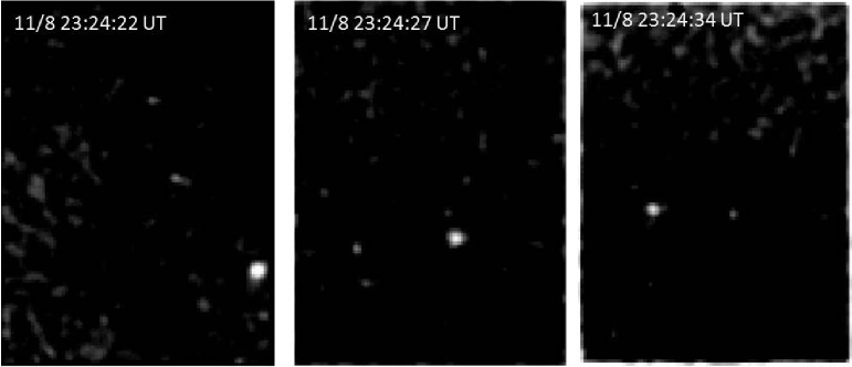
Figure 1: Mid-infrared images of 2005 YU₅₅ obtained by the miniTAO/MAX38 camera in the 18.7 $\mu$m filter during the time of the closest Earth approach. North is up and west is right. The asteroid moved from right (west) to left (east).

We observed the asteroid 2005 YU₅₅ in the period Nov. 8 - 10, 2011 with the mid-infrared camera MAX38 (Miyata et al. miyata08 (2008); Nakamura et al. nakamura10 (2010); Asano et al. asano12 (2012)) attached on the mini-TAO 1 meter telescope (Sako et al. sako08 (2008)) which is located at 5640 m altitude on the summit of Co. Chajnantor in Chile, which is part of the University of Tokyo Atacama Observatory Project (PI: Yuzuru Yoshii; Yoshii et al. yoshii10 (2010)). MAX38 has a 128$\times$128 Si:Sb BIB detector with a pixel scale of 1.26 arcsec and a field of view of 2$\times$2.5 arcmin determined by the rectangular field stop in the cold optics (the remaining 0.5$\times$2.5 arcmin of the detector array is used for spectroscopy). The MAX38 observing periods (2011-Nov-08 23:04 to Nov-09 01:51 UT and from Nov-09 23:56 to Nov-10 02:04 UT) covered the time of the closest approach (2011-Nov-08 23:24 UT) and about 24 hours later. The weather conditions were excellent through the observations. Imaging observations in the 8.9 $\mu$m ($\Delta\lambda$ $\sim$ 0.9 $\mu$m), 12.2 $\mu$m (0.5 $\mu$m), and 18.7 $\mu$m (0.9 $\mu$m) bands were carried out. $\alpha$ Tuc (IRAS22150-6030, HR 8502, HD 211416) was also observed after the observations of the asteroid as a flux standard. The absolute flux value of the standard star was obtained via the $\alpha$ Tuc template spectrum (Cohen et al. cohen99 (1999)).

Since the distance to the asteroid from the Earth was very short, the asteroid had a very high apparent motion on the sky. We pointed the telescope at repeated intervals to follow the asteroid’s movement. The intervals were set to 1 minute and 3 minutes on Nov. 8 and 9, respectively. Normal sidereal tracking was applied in the period between the telescope pointings. Images were taken at a frame rate of 3.8 Hz with an effective integration time of 0.197 sec. The frame rate is fast enough not to extend the image of the asteroid on each frame. Chopping technique was not applied because background can be canceled out with using frames just before or after an object frame. The observation parameters are summarized in Table 1 and three examples of reduced images taken at the time of the closest approach are shown in Fig. 1.

Table 1: MAX38 Observation Parameters. The first period includes the closest Earth approach.

2011-Nov-.. (UT)		Filter	# of	airmass-range
Day Start	End	Band	frames	2005 YU55	$\alpha$ Tuc
08 23:04	00:15	18.7	20196	1.31-1.47	1.41-1.48
09 00:30	00:41	8.9	2550	1.51-1.55	1.29
09 01:11	01:24	12.2	1734	1.65-1.70	1.31
09 23:56	00:50	18.7	12288	2.00-1.61	1.53-1.64
10 01:38	02:04	8.9	4928	1.43-1.38	1.67

On Nov. 8, the asteroid was so bright (observatory-centric distance was about 0.0021-0.0023 AU) that it was detectable in each frame. Sky frames -composed by averaging 7 frames taken within 2 sec- were subtracted. This successfully canceled out sky variation similar to observations taken in chopping technique. Aperture photometry with an aperture radius of 3 arcsec was applied for each frame. Photometric values were determined by averaging frames taken in a period of 5 minutes. Errors were estimated as standard deviation of the photometric values.

On Nov. 9 the asteroid was already at about 0.0084-0.0089 AU distance and it was difficult to detect the asteroid on each frame. Here, we added 92 frames into one image by shifting the frames to compensate the asteroid’s movement on the sky and subtracted the averaged sky frames. The frame-to-frame shifts were calculated from the ephemeris provided by the NASA Horizons web page. The asteroid images in the co-added frames appeared nearly point-like and no noticeable extensions were detected. We applied aperture photometry on the final sky-subtracted images. The final flux and error values were again obtained by averaging all individual photometric values.

In addition to the photometric error we also added a 5% absolute flux calibration error for the N-band data and a 7% error for the Q-band data based on the radiometric tolerance discussion in Cohen et al. (cohen99 (1999)) and the information given in the stellar template. These errors also include possible colour-terms (estimated to be below 2%) due to the different spectral shapes of the star and the asteroid in the N- and Q-band filters. In the first night (8/9 Nov.) $\alpha$ Tuc and the asteroid were observed at similar airmass and similar PWV-levels (based on APEX measurements) and no additional corrections were needed. In the second night (9/10 Nov.) 2005 YU₅₅ was observed in Q-band at a large airmass close to 2.0 and a PWV of around 0.5 mm, while $\alpha$ Tuc was taken at an airmass of around 1.6 and a PWV-level of about 0.3 mm. Based on ATRAN model calculation of the atmospheric transmittance vs. PWV for the 18 $\mu$m filter we estimated that the derived Q-band flux for 2005 YU₅₅ must be about 5-10% too low. We increased the derived 18.7 $\mu$m flux of the second night by 8% and gave a 10% absolute flux calibration error (instead of 7%) to compensate for the additional source of uncertainty. The final calibrated flux densities are given in Table 2.

Table 2: Observing geometries (miniTAO-centric) and final calibrated flux densities. Negative phase angles: after opposition (object was trailing the Sun). An absolute flux calibration of 5% (N-band) and 7/10% (1^st/2^nd day Q-band) has been added. The second day Q-band data point has been corrected for airmass/PWV effects (see text).

Julian Date	$\lambda_{ref}$	FD	FDerr	rhelio	$\Delta_{obs}$	$\alpha$	Observatory/
mid-time	[$\mu$m]	[Jy]	[Jy]	[AU]	[AU]	[deg]	Instrument
2455874.46285	18.7	189.53	30.44	0.9904028	0.0021426484	-97.17	miniTAO/MAX38
2455874.46632	18.7	192.82	30.25	0.9904293	0.0021415786	-96.46	miniTAO/MAX38
2455874.46979	18.7	192.81	29.53	0.9904558	0.0021408565	-95.74	miniTAO/MAX38
2455874.47326	18.7	196.73	32.07	0.9904823	0.0021404827	-95.03	miniTAO/MAX38
2455874.47674	18.7	194.37	33.12	0.9905088	0.0021404572	-94.32	miniTAO/MAX38
2455874.48021	18.7	203.01	32.83	0.9905352	0.0021407803	-93.61	miniTAO/MAX38
2455874.48368	18.7	204.71	35.25	0.9905617	0.0021414518	-92.89	miniTAO/MAX38
2455874.48715	18.7	212.57	34.45	0.9905882	0.0021424716	-92.18	miniTAO/MAX38
2455874.49062	18.7	217.57	33.65	0.9906147	0.0021438391	-91.47	miniTAO/MAX38
2455874.49410	18.7	223.70	34.04	0.9906411	0.0021455542	-90.76	miniTAO/MAX38
2455874.49757	18.7	219.77	32.97	0.9906676	0.0021476157	-90.05	miniTAO/MAX38
2455874.50104	18.7	222.79	32.28	0.9906941	0.0021500229	-89.34	miniTAO/MAX38
2455874.50451	18.7	222.34	34.22	0.9907206	0.0021527749	-88.63	miniTAO/MAX38
2455874.50799	18.7	227.06	34.94	0.9907471	0.0021558704	-87.93	miniTAO/MAX38
2455874.51146	18.7	223.24	35.74	0.9907735	0.0021593083	-87.22	miniTAO/MAX38
2455874.52187	8.9	126.81	15.22	0.9908530	0.0021716598	-85.13	miniTAO/MAX38
2455874.52535	8.9	123.50	13.45	0.9908794	0.0021764507	-84.43	miniTAO/MAX38
2455874.52882	8.9	124.36	14.10	0.9909059	0.0021815751	-83.74	miniTAO/MAX38
2455874.54965	12.2	225.22	24.78	0.9910648	0.0022191984	-79.67	miniTAO/MAX38
2455874.55312	12.2	221.94	24.94	0.9910912	0.0022265916	-79.00	miniTAO/MAX38
2455874.55660	12.2	215.43	23.59	0.9911177	0.0022342979	-78.34	miniTAO/MAX38
2455874.56007	18.7	261.49	37.68	0.9911442	0.0022423147	-77.68	miniTAO/MAX38
2455874.56354	18.7	253.99	33.16	0.9911706	0.0022506389	-77.03	miniTAO/MAX38
2455874.56701	18.7	248.50	34.51	0.9911971	0.0022592671	-76.38	miniTAO/MAX38
2455874.57049	18.7	247.40	33.88	0.9912236	0.0022681963	-75.74	miniTAO/MAX38
2455874.57396	18.7	241.90	36.31	0.9912501	0.0022774233	-75.10	miniTAO/MAX38
2455874.57743	18.7	241.30	33.92	0.9912765	0.0022869445	-74.47	miniTAO/MAX38
2455875.51458	18.7	28.08	5.90	0.9983930	0.0084376885	-19.23	miniTAO/MAX38
2455875.57639	8.9	19.60	2.32	0.9988611	0.0089028990	-18.57	miniTAO/MAX38

2.2 Space far-infrared observations with Herschel-PACS

The far-infrared observations with the Herschel space observatory were reported by Müller et al. (2011b ). 2005 YU₅₅ crossed the entire visibility window ($\sim$60^∘ to $\sim$115^∘ solar elongation) in about 16 hrs and its apparent motion was between 2.8 and 3.8 ^∘/h, far outside the technical tracking limit of the satellite. Therefore, we performed two standard scan-map observations of 240 s length each -one in the 70/160 $\mu$m (2011-Nov-10 14:52-14:56 UT, OBSID 1342232729) and one in the 100/160 $\mu$m filter combination (2011-Nov-10 14:57-15:01 UT, OBSID 1342232730)- at fixed times at pre-calculated positions on the sky. Each scan-map consisted of 4 scan-legs of 14 arcmin length and separated by 4 arcsec parallel to the apparent motion of the target and with a scan-speed of 20^′′/s. During both scan-map observations 2005 YU₅₅ crossed the observed field-of-view and the target was seen in each scan-leg. Figure 2 (top) shows the sky-projected image of the 70 $\mu$m band observations. The PACS photometer takes data frames with 40 Hz, but binned onboard by a factor of 4 before downlink. We re-centered/stacked all frames where the satellite was scanning with constant speed (about 1700 frames in each of the two dual-band measurements) on the expected position of 2005 YU₅₅. The results are shown in Fig. 2 (bottom). This technique worked extremely well and one can clearly see many details of the tripod-dominated point-spread-function. We performed aperture photometry on the final calibrated images and estimated the flux error via photometry on artificially implemented sources in the clean vicinity around our target. The fluxes were finally corrected for colour terms to obtain monochromatic flux densities at the PACS reference wavelengths. These corrections are due to the differences in spectral energy distribution between 2005 YU₅₅ and the assumed constant energy spectrum $\nu$ F_ν = const. in the PACS calibration scheme. The colour-corrections for objects in the temperature range of $\approx$ 250 - 400 K are 1.01, 1.03, 1.06 ($\pm$ 0.01) in blue, green, red band respectively. The photometric error of the artificial sources were combined quadratically with the absolute flux calibration errors (5% in all 3 bands based on the model uncertainties of the fiducial stars used in the PACS photometer flux calibration scheme) and the error related to the colour-correction (1%). The final monochromatic flux densities and their absolute flux errors at the PACS reference wavelengths 70.0, 100.0 and 160.0 $\mu$m are listed in Table 3.

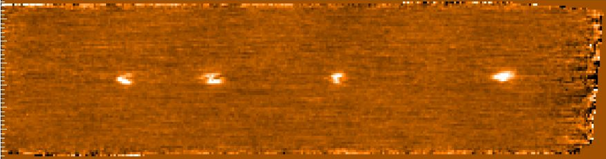
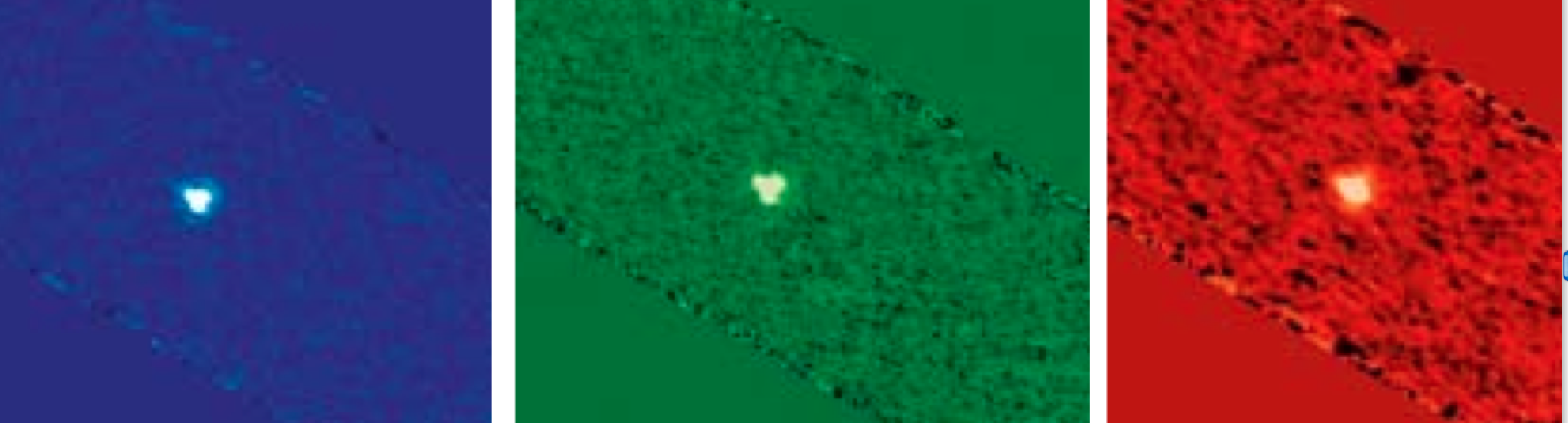
Figure 2: Top: Sky-projected PACS image of 2005 YU₅₅ at 70 $\mu$m. Each of the 4 scan-legs has seen the target at a different position. Bottom: object-centered images of the target in the 3 filters: blue (70 $\mu$m), green (100 $\mu$m), red (160 $\mu$m). The tripod-dominated point-spread-function is clearly visible.

Table 3: Observing geometries (Herschel-centric) and final calibrated flux densities. Negative phase angles: after opposition.

Julian Date	$\lambda_{ref}$	FD	FDerr	rhelio	$\Delta_{obs}$	$\alpha$	Observatory/
mid-time	[$\mu$m]	[Jy]	[Jy]	[AU]	[AU]	[deg]	Instrument
2455876.120565	70.0	12.35	0.63	1.002978	0.005403	-70.88	Herschel-PACS
2455876.120565	160.0	2.55	0.13	1.002978	0.005403	-70.88	Herschel-PACS
2455876.124075	100.0	6.87	0.35	1.003004	0.005415	-70.62	Herschel-PACS
2455876.124075	160.0	2.66	0.14	1.003004	0.005415	-70.62	Herschel-PACS

2.3 Groundbased millimeter observations with the SMA

Table 4: Observing geometries (SMA-centric) and final calibrated flux densities. Negative phase angles: after opposition.

Julian Date	$\lambda_{ref}$	FD	FDerr	rhelio	$\Delta_{obs}$	$\alpha$	Observatory/
mid-time	[$\mu$m]	[Jy]	[Jy]	[AU]	[AU]	[deg]	Instrument
2455874.95042	1328.9	0.075	0.020	0.9941165	0.0042883	-34.66	SMA/230 GHz receiver

We performed observations of 2005 YU₅₅ a few hours past closest Earth approach on Nov. 9, 2011 using the Submillimeter Array (SMA) located near the summit of Mauna Kea in Hawaii. The SMA was operated in separated sideband mode with 2ĠHz continuum bandwidth per sideband. The lower sideband was tuned to 220.596 GHz and the upper sideband (USB) at 230.596 GHz, providing a mean frequency of 225.596 GHz, or 1328.9 $\mu$m (covering the range from 1300.1 to 1359.0 $\mu$m). Complex gains were obtained from several different quasars as the asteroid moved across the sky. The amplitude scale was corrected for Earth atmospheric opacity through standard system temperature calibration, and then corrected to the absolute (Jansky) scale by referencing to observations of Uranus and Callisto, astronomical sources with flux densities known to within $\sim$5% at this frequency.

The measurements were difficult due to poor weather, particularly atmospheric phase stability, and were further hampered by the exceptionally rapid motion of the object. The asteroid’s apparent position at its fastest changed by $\sim$7^′′/s relative to sidereal, which is significantly faster than the SMA phase tracking system (the digital delay software, or DDS) was designed for. To compensate, a special version of the DDS was created which attempted to track the phase on much shorter timescales. However, this was only partly successful and there were obvious signs of decorrelation (loss of signal caused by the motion of the source relative to the tracked phase center) on most baselines. This required extensive data flagging and secondary self-calibration of the amplitude, which introduced significant systematic error in the flux density scale.

Despite these challenges, we obtained a clear detection of the object. Figure 3 shows the 1.3 mm image of 2005 YU₅₅ after both phase reference calibration and further self-calibration. The target itself was unresolved and the oblong image of the asteroid in Figure 3 is simply due to the PSF of the instrument for the observations, which is shown in the lower left corner as an ellipse of 3.73^′′ $\times$ 2.58^′′ in size, with a major axis position angle of 83.66^∘ East of North. Over the 3.5 hours of observation (UT Nov 9, 2011 09.16 - 12.46 hrs) we further see the expected drop in flux density as the source recedes, consistent with the apparent size decrease with time. While the detection is of high signficance (SNR $\sim$35), the systematic problems of compensating for the tracking-induced decorrelation along with the poor weather dominated the flux-density error budget. Taking all effects into account we obtained a flux density of 75 $\pm$ 25 mJy at observation mid-time (UT Nov 9, 2011 10:49, see Tbl. 4).

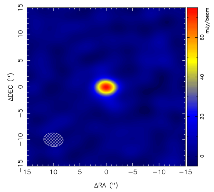
Figure 3: SMA image of 2005 YU₅₅ at 1.3 mm. The ellipse represents the 2-dimensional full width at half maximum of the synthesized beam of the array, which is effectively the PSF of the instrument for the observations of an unresolved target.

2.4 Auxiliary datasets

Radar measurements.

Nolan et al. (nolan10 (2010)), Busch et al. (busch12 (2012)) and Taylor et al. (2012a ; 2012b ) presented results obtained by radar measurements using the Arecibo S-band, the Deep Space Network Goldstone DSS-14 and DSS-13, Green Bank Telescope and Arecibo/VLBA (radar speckle tracking). They found 2005 YU₅₅ to be a dark (at radar/radio wavelengths), spherical object of about 400 m diameter and a rotation period of roughly 18 hrs (Nolan et al. nolan10 (2010); Taylor et al. 2012a ). Busch et al. (busch12 (2012)) confirmed the nearly spheroidal shape and determined the maximum dimensions of the object to be 360 $\pm$ 40 m in all directions. The radar team estimated the pole direction from the motion of the radar speckle pattern during three days of observations after the flyby. Combining the radar images and the speckle data excluded all prograde pole directions, and restricted the possible retrograde poles to ($\lambda_{ecl}$, $\beta_{ecl}$) = (20^∘, -74^∘) $\pm$ 20^∘ with a rotation period of 19.0 $\pm$ 0.5 hrs and consistent with a principle-axis rotation.

Thermal infrared observations from Gemini-North/Michelle.

Lim et al. (2012a ; 2012b ) obtained thermal infrared photometry and spectroscopy in N- and Q-band using the Michelle instrument at Gemini-North. According to their thermal model analysis (T_ss = 360 - 370 K; $\eta$ $\approx$ 1.25-1.5) the thermal measurements are consistent with an object diameter of 400 m, but the best fit to their data was found for a size of 322 $\pm$ 18 m and a maximum subsolar temperature T_ss of 409 $\pm$ 12 K (thermal model $\eta$ $\approx$ 0.93). More recently, Lim et al. (2012c ) combined their thermal data with results from radar measurements and find now an equatorial diameter of 380 $\pm$ 20 m and a thermal inertia $\Gamma$ $\approx$ 500 - 1500 Jm^-2s^-0.5K^-1. They also calculated values for the effective diameter via radiometric techniques and based only on their thermal data. They found an effective diameter of 310 m for a low thermal inertia of 350 Jm^-2s^-0.5K^-1 and of 350 m for a thermal inertia of 1000 Jm^-2s^-0.5K^-1 (DPS meeting #44, #305.01 presentation).

Keck adaptive-optics (AO) imaging.

Merline et al. (merline11 (2011); merline12 (2012)) reported on adaptive optics (AO) imaging of 2005 YU₅₅ during its close fly-by on 2011 Nov 9 UT with the Keck II AO system NIRC2. The preliminary results were derived under the assumption of a smooth triaxial ellipsoid having a principle-axis rotation of 18 hr. They found a preference for poles in the southern sub-latitudes and an effective object diameter of 307 $\pm$ 15 m. This would be consistent with the radar-favoured retrograde sense of rotation meaning that the object presented a warm terminator during its close approach. In addition, they give two explicit solutions: (a) prograde pole with ($\lambda_{ecl}$, $\beta_{ecl}$) = (339^∘, +84^∘) $\pm$ 6^∘ and object dimensions of 337 $\times$ 324 $\times$ 267 m ($\pm$ 15 m in each dimension), corresponding to a spherical equivalent diameter of 308 $\pm$ 9 m; (b) retrograde pole with ($\lambda_{ecl}$, $\beta_{ecl}$) = (22^∘, -35^∘) $\pm$ 15^∘ and object dimensions of 328 $\times$ 312 $\times$ 245 m ($\pm$ 15, 15, 30 m) corresponding to a spherical equivalent diameter of 293 $\pm$ 14 m.

VLT-NACO speckle imaging observations.

Sridharan et al. (sridharan12 (2012)) performed VLT-NACO speckle imaging in Ks band in no-AO mode. The observations on 2005 YU₅₅ were carried out one hour (10-min block) and two hours (15-min block) after the closest Earth approach, interleaved by sky background and calibration observations. The planned closed-loop AO observations failed due to poor observing conditions and only no-AO mode (speckle imaging mode) observations were possible. They found that 2005 YU₅₅ has a spherical shape with a mean diameter of about 270 m. At the same time they extracted a mean diameter of 261$\pm$20 m $\times$ 310$\pm$30 m from edge-enhanced image reconstructions. The large uncertainties are due to the theoretical resolution of 95 m at the distance of the object and the final image quality.

CCD photometric observations.

CCD lightcurve measurements from different observers were analysed by Warner et al. (2012a ; 2012b ). Their analysis resulted in two possible synodic periods of 16.34 $\pm$ 0.01 h with an amplitude of 0.24 $\pm$ 0.02 mag (9-17 Nov, 2011) and 19.31 $\pm$ 0.02 h with an amplitude of 0.20 $\pm$ 0.02 mag. The first one was apparently supported by the initial radar analysis, while the second one is now the currently favoured solution by the radar team. The 19.31 h lightcurve has a bimodal shape and there seem to be indications for a non-principal axis rotation. Due to a large phase angle coverage of the CCD data they were also able to derive the absolute R-band magnitude H_R = 20.887 $\pm$ 0.042 and the phase slope parameter G = -0.147 $\pm$ 0.014. With an assumed V-R value of 0.38 they calculated the absolute V-band magnitude H_V = 21.27 $\pm$ 0.05.

Absolute magnitude and phase curve.

Based on Bessel R-band photometry and long-slit CCD spectrograms during the 2010 and 2011 apparitions, Hicks et al. (hicks10 (2010); hicks11 (2011)) reported an absolute R-band magnitude of H_R = 20.73 and a phase slope parameter G = -0.12 describing a very steep phase curve which is typically found for low-albedo C- and P-type asteroids. They measured a V-R colour of 0.37 mag leading to an absolute V-band magnitude of H_V = 21.1 $\pm$ 0.1. An indpendent work by Bodewits et al. (bodewits11 (2011)) presented a V-band absolute magnitude of H_V = 21.2 when applying a phase curve derived from UV measurements (G_UV = -0.13).

3 Thermophysical model analysis

For the analysis of our thermal data (miniTAO/MAX38, SMA, Herschel/PACS) we applied a thermophysical model (TPM) which is based on the work by Lagerros (lagerros96 (1996); lagerros97 (1997); lagerros98 (1998)). This model is frequently and successfully applied to near-Earth asteroids (e.g., Müller et al. mueller04b (2004); Müller et al. mueller05 (2005); Müller et al. 2011a ; Müller et al. mueller12 (2012)), to main-belt asteroids (e.g., Müller & Lagerros mueller98 (1998); Müller & Blommaert mueller04a (2004)), and also to more distant objects (e.g. Horner et al. horner12 (2012); Lim et al. lim10 (2010)). The TPM takes into account the true observing and illumination geometry for each observational data point, a crucial aspect for the interpretation of our 2005 YU₅₅ observations which cover a wide range of phase angles. The TPM allows to specify a shape model and spin-vector properties. The heat conduction into the surface is controlled by the thermal inertia $\Gamma$. The observed mid- and far-IR fluxes are connected to the hottest regions on the asteroid surface and dominated by the diurnal heat wave. The seasonal heat wave is less important and therefore not considered here. The infrared beaming effects are calculated via a surface roughness model, described by segments of hemispherical craters. Here, mutual heating is included and the true crater illumination and the visibility of shadows is considered. The level of roughness is driven by the r.m.s. of the surface slopes which correspond to a given crater depth-to-radius value combined with the fraction of the surface covered by craters, see also Lagerros (lagerros96 (1996)) for further details. We used a constant emissivity of 0.9 at all wavelengths, knowing that the emissivity can decrease beyond $\sim$200 $\mu$m in some cases (e.g., Müller & Lagerros mueller98 (1998); mueller02 (2002)). All of our data -except the SMA data point which has a large errorbar- have been taken at wavelength $<$200 $\mu$m and the constant emissivity is therefore a valid assumption. The TPM input parameters and applied variations are listed in Table. 5.

Table 5: Summary of general TPM input parameters and applied ranges.

Param.	Value/Range	Remarks
$\Gamma$	0…3000	J m-2 s-0.5 K-1, thermal inertia
		(25 values spread in log-space)
$\rho$	0.1…0.8	r.m.s. of surface slopes, steps of 0.1
$f$	0.6	surface frac. covered by craters
$\epsilon$	0.9	$\lambda$-independent emissivity
$H_{\rm{V}}$-mag.	21.2 $\pm$ 0.15 mag	average of published values
G-slope	-0.13 $\pm$ 0.02	average of published values
shape	spherical/ellipsoidal	info from radar and AO
Psid [h]	16.34 h; 19.31 h	Warner et al. (2012a ; 2012b )
spin-axis	(20.0∘, -74.0∘) $\pm$ 20∘	Busch et al. (busch12 (2012))
($\lambda_{ecl}$,$\beta_{ecl}$)	(339.0∘, +84.0∘) $\pm$ 6∘	Merline et al. (merline11 (2011); merline12 (2012))
	(22.0∘, -35.0∘) $\pm$ 15∘	Merline et al. (merline11 (2011); merline12 (2012))
	(309.3∘, +89.5∘)	obliquity 0∘ (prograde)
	(129.3∘, -89.5∘)	obliquity 180∘ (retrograde)
	(337.2∘, -13.9∘)	pole-on case1 for Herschel obs.
	(157.2∘, +13.9∘)	pole-on case2 for Herschel obs.
	(273.0∘, +1.7∘)	pole-on case1 for TAO/MAX38
	(93.0∘, -1.7∘)	pole-on case2 for TAO/MAX38
	(337.2∘, +76.1∘)	equ.-on case1 for Herschel obs.
	(157.2∘, -76.1∘)	equ.-on case2 for Herschel obs.
	(273.0∘, -88.3∘)	equ.-on case1 for TAO/MAX38
	(93.0∘, +88.3∘)	equ.-on case2 for TAO/MAX38
	(0/90/180/270∘, $\pm$60∘)	intermediate orientations
	(0/90/180/270∘, $\pm$30∘)	intermediate orientations
	(0/90/180/270∘, 0∘)	pole in ecliptic plane

3.1 Using a spherical shape model

We started our analysis with a spherical shape model to see which spin-axis orientations, sizes, geometric albedos, and thermal properties produce acceptable solutions with reduced $\chi^{2}$-values around or below 1.0. For the spin-axis solutions we used all values specified in literature and many additional orientations to cover the entire $\lambda_{ecl}$-$\beta_{ecl}$ space. For the calculation of the reduced $\chi^{2}$-curves we consider the true observing and illumination constellation (helio-centric and observer-centric distances, phase angle, spin-axis orientation) for each epoch and then we compare with the corresponding measurement. These calculations are done for a wide range of thermal inertias and different levels of surface roughness as specified in Table 5. An example for the application of this technique can be found in Müller et al. (2011a ). Each model setup produces a curve of reduced $\chi^{2}$-values as a function of thermal inertia. Figure 4 shows these curves for all different spin-axis orientation, a rotation period of 19.31 h and an intermediate level of surface roughness (r.m.s. of surface slopes of 0.3). Reduced $\chi^{2}$-values around or below 1.0 correspond to TPM solutions which explain all observed fluxes in a statistically acceptable way. There are several spin-axis orientations which produce an excellent match to all our thermal measurements at thermal inertia values in the range between approximately 200 and 1500 Jm^-2s^-0.5K^-1.

Figure 4: Calculation of reduced $\chi^{2}$-values for all specified spin-axis orientations, a fixed rotation period of 19.31 h and an intermediate surface roughness level (r.m.s. of surface slopes of 0.3). The prograde AO solution (solid line) and the radar solution (dashed line) for the spin-vector are indicated in the figure.

The distribution of the reduced $\chi^{2}$-minima along the ecliptic longitudes and latitudes is shown in Figure 5. There are large zones in the $\lambda_{ecl.}$-$\beta_{ecl}$-space which can be excluded with high probability (light blue, green, yellow, red zones), but there remain several possible spin-axis orientations compatible with our dataset (dark blue zones), including the radar and AO solutions.

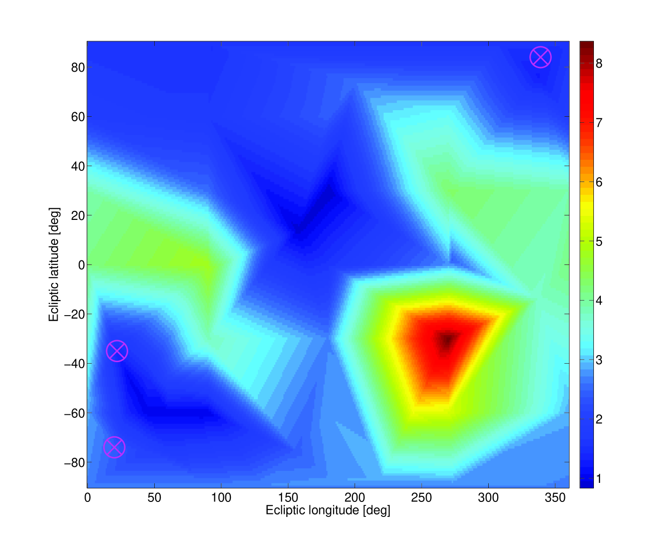
Figure 5: The $\chi^{2}$-minima calculated for all spin-axis orientations listed in Table 5 and for an intermediate level of roughness (r.m.s.slope 0.3). The dark blue zones indicate spin-poles which allow us to obtain an acceptable match to all thermal data simultaneously (reduced $\chi^{2}$-values around or below 1.0). The radar and both AO solutions are indicated by the crossed circles. Note that the size, albedo and thermal inertia are free parameters and only the best possible solution for each spin-axis has been considered.

Both figures (Figs. 4 & 5) have a slight dependency on the selected surface roughness (for both figures we have used r.m.s. of surface slopes of 0.3). In general, lower roughness (r.m.s. of surface slopes at 0.1) produces lower $\chi^{2}$-minima and at smaller thermal inertia values going down to about 200 Jm^-2s^-0.5K^-1. Higher values for the surface roughness (r.m.s. of surface slopes of $\geq$0.5) shift the $\chi^{2}$-minima to values well above 1.0 and towards higher thermal inertia going up to about 1500 Jm^-2s^-0.5K^-1. It is interesting to note that the prograde AO solution (solid line in Fig. 4) works very well ($\chi^{2}$-minima very close to 1.0) for a low surface roughness, while the radar solution produces a better match in case of a high surface roughness.

3.2 Influence of the spin-axis orientation

As a next step, we investigate the influence of different spin-axis orientations on the size and albedo solutions. We determined the $\chi^{2}$-minima for all listed spin-axis orientations and for four different levels of roughness (r.m.s. of surface slopes at 0.1, 0.3, 0.5 and 0.8). Figure 6 shows how the corresponding radiometric sizes and geometric albedos are distributed in the reduced $\chi^{2}$-picture. We connected the four $\chi^{2}$-minima belonging to the AO-solution (solid line) and the ones belonging to the radar solution (dashed line) in Fig. 6. These lines show that the connected size and albedo values remain stable, just the fit gets better (lower $\chi^{2}$-minima) for specific roughness settings. We also found that the derived thermal inertias change significantly with roughness at similar $\chi^{2}$-values, indicating that we cannot resolve the degeneracy between roughness and thermal inertia with our dataset. A smoother surface is connected to lower values for the thermal inertia, the rougher surfaces require higher thermal inertias.

Figure 6: The distribution of the $\chi^{2}$-minima and the related effective diameter (top) and geometric albedos (bottom). The four different levels of roughness are indicated by different symbols. The values for the prograde AO solution (solid line) and the radar solution (dashed line) are connected in the figures.

The thermal data are compatible with different spin-axis orientations, but the size, the geometric albedo and also the possible thermal inertias are very well constrained by our thermal dataset. The best solutions are found for an effective diameter of about 310 m, if we include the best solutions for the prograde AO spin-axis and the radar spin-axis orientations, then the possible diameter range goes from 295 to 335 m (see Fig. 6, top). For the geometric albedo we find a value of about 0.062 and a possible range between 0.053 to 0.067 (see Fig. 6, bottom). Figure 7 shows how our best TPM solution translates the insolation during the epoch of the Herschel measurement into a thermal picture of the surface as seen from Herschel. For the calculations we used a spin-axis orientation of ($\lambda_{ecl}$, $\beta_{ecl}$) = (60^∘, -60^∘) and a spherical shape model with a total of 800 facets. The large influence of the thermal inertia in combination with the object’s rotation is the reason for the warm temperatures also in regions without direct illumination.

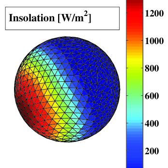
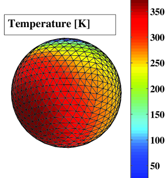
Figure 7: TPM picture of 2005 YU₅₅ as seen from Herschel on 2011-Nov-10 14:55 UT in the object-centered reference frame (z-axis along the object’s rotation axis) and with the Sun at a phase angle of -71^∘, spin-axis orientation: ($\lambda_{ecl}$, $\beta_{ecl}$) = (60^∘, -60^∘), spherical shape model with a total of 800 facets. Top: insolation in W/m². Bottom: temperature in K.

4 Discussions

4.1 Comparison with the radar results

The comparison between the radar results (Busch et al. busch12 (2012)) and our findings is very interesting. If we use the radar diameter (360 $\pm$ 40 m, close to a spheroidal shape) and the spin-axis properties ([$\lambda_{ecl}$, $\beta_{ecl}$] = [20^∘, -74^∘] $\pm$ 20^∘, P_sid = 19.0 $\pm$ 0.5 h) it is not possible to find an acceptable match to our thermal measurements. The reduced $\chi^{2}$-minima stay always well above 2.0 and the match between TPM-predictions and observed fluxes is very poor. Even for the lowest diameter limit of 320 m the model calculations would exceed the measured fluxes systematically by 15-25%. At a diameter of 360 m the model fluxes are already 30-40% above the measurements. The radar size estimates are -as the radiometric size estimates- model dependent. The spin-axis orientation as well as the rotation rate have a larger influence on the radar solution (e.g., Ostro et al. ostro02 (2002)) than they have on the radiometric solution. The radar images are dominated by the surface part which is closest to the antenna while the thermal data are tidely connected to the entire cross-section at the moment of observation. This might explain the differences between both techniques.

However, we do find an acceptable match to all thermal data if we just use the radar spin-properties combined with a high level of surface roughness (r.m.s. of surface slopes of 0.8). But the corresponding diameter is only 299 m -well outside the radar derived range- with a p_V=0.067 and a thermal inertia of 400 Jm^-2s^-0.5K^-1. In fact, all high obliquity cases with $\beta_{ecl}$ $\leq$ -60^∘ (retrograde sense of rotation) produce small diameters in the range 300-310 m, while only the low obliquity cases with $\beta_{ecl}$ $\geq$ +60^∘ (prograde sense of rotation) produce larger effective diameters of 325-340 m.

4.2 Comparison with AO and speckle results

The Keck AO results presented by Merline et al. (merline12 (2012)) compare better with our findings. Table 6 summarises the AO and our radiometric results.

Table 6: Comparison between AO results and our findings.

sense of	spin-axis	AO-size	AO Dequ	TPM-Dequ
rotation	($\lambda_{ecl}$, $\beta_{ecl}$)	[m]	[m]	[m]
prograde	339∘, +84∘	337$\times$324$\times$267	308 $\pm$ 9	333
retrograde	22∘, -35∘	328$\times$312$\times$245	293 $\pm$ 14	299
retrograde	southern poles		307 $\pm$ 15	300-310

The southern rotational poles are not specified in detail by Merline et al. (merline12 (2012)), but here we see for the first time an agreement between the derived sizes. The originally specified retrograde pole towards an ecliptic latitude of -35^∘ is very unlikely: acceptable TPM solutions (with reduced $\chi^{2}$-minima below 2.0) are only found if the thermal inertia would be well above 2000 Jm^-2s^-0.5K^-1, an unrealistically high value which has never been measured before. It should be noted here that the highest derived thermal inertias are still below 1000 Jm^-2s^-0.5K^-1 (e.g., Delbo et al. delbo07 (2007)) and that our mid- to far-IR data originate in the top layer on the surface. We don’t see any signatures of sub-surface layers where the thermal inertia could be significantly higher (Keihm et al. keihm12 (2012)).

The speckle observation in no-AO mode presented by Sridharan et al. (sridharan12 (2012)) revealed a roughly spheroidal shape with a mean diameter of 270 m. By using a more sophisticated reconstruction technique they estimated a mean diameter of 261 $\pm$ 20 m $\times$ 310 $\pm$ 30 m, corresponding to an object-averaged size of approximately 285 $\pm$ 25 m. Within the errorbars, this value agrees with our radiometrically derived diameter of 300-310 m and it also creates doubts if the large radar size is realistic. The indications for a diameter close to 300 m makes also the various prograde solutions more unlikely, which all require diameters in the range 325-340 m.

4.3 Spin-axis properties

Combining the spin-axis information given by Busch et al. (busch12 (2012)), Merline et al. (merline12 (2012)) and our findings (see Fig. 4), our analysis supports a retrograde sense of rotation with a possible spin-axis orientation of ($\lambda_{ecl}$, $\beta_{ecl}$) = (60^∘ $\pm$ 30^∘, -60^∘ $\pm$ 15^∘). The relatively large errors in ($\lambda_{ecl}$, $\beta_{ecl}$) are covering also the possible solutions connected to the different roughness levels mentioned before. If we use this solution, then the size estimate from AO observations matches our radiometrically derived optimal size and we also have an agreement with the radar derived spin-pole. The discrepancy with the radar size remains.

Our thermal observations cover a wide range of phase angles, wavelengths and different illumination and observing geometries. This allowed us to exclude many spin-axis orientations (see Fig. 5). Nevertheless, we could not find a strong preference for a single spin-axis orientation nor for the sense of rotation. Even very extreme solutions like the retrograde radar solution and the prograde AO solution seem to explain the data equally well. This is very surprising. Based on our previous modeling experiences for 1999 JU₃ (Müller et al. 2011a ) and 1999 RQ₃₆ (Müller et al. mueller12 (2012)) based on much smaller sets of thermal data, we expected to find a unique spin-axis solution. But this might be an indication that 2005 YU₅₅ is a tumbler with a strongly time-dependent orientation of the spin-axis (for further details on tumbling asteroids see Pravec et al. pravec05 (2005)). Busch et al. (busch12 (2012)) speculated already about the possibility that terrestrial tides might have torqued the object into a non-principal axis spin state. However, their observations are consistent with a principle-axis rotation. Warner et al. (2012b ) found two, non-commensurate solutions for the rotation period (16.34 $\pm$ 0.01 h; 19.31 $\pm$ 0.02 h) which they could not fully explain. They suggest that a non-principal axis rotation should be considered. After the radar and lightcurve analysis, the thermal analysis is now also pointing towards the possibility of a non-principle axis rotation.

We also looked into the influence of the two published rotation periods. But the $\approx$3 h difference between the two available periods did not affect our radiometric solutions significantly. The longer rotation period is typically requiring slightly higher inertias to produce the same disk-integrated flux, but this is a marginal effect here in this case.

4.4 Comparison with other thermal measurements

Instead of comparing our TPM radiometric results with the preliminary results produced by Lim et al. (2012a ; 2012b ; 2012c ) via a simple thermal model, we predicted flux densities for the epochs and the wavelength bands of the Michelle/Gemini North observations shown in Figure 2 in Lim et al. (2012b ). For the TPM prediction we simply used our best effective diameter (310 m) and albedo (p_V = 0.062) solution connected to our preferred spin-axis orientation of ($\lambda_{ecl}$, $\beta_{ecl}$) = (60^∘, -60^∘). The thermal inertia and roughness levels are less well constrained and our dataset does not allow to break the degeneracy between these two parameters. A low roughness (r.m.s. of surface slopes = 0.1) combined with small values of the thermal inertia of about 200 Jm^-2s^-0.5K^-1 would explain our measurements as well as higher roughness levels (r.m.s. of surface slopes = 0.5) combined with higher thermal inertia around 800 Jm^-2s^-0.5K^-1. We selected an intermediate solution (r.m.s. of surface slopes = 0.3; thermal inertia = 500 Jm^-2s^-0.5K^-1).

The Gemini-North/Michelle photometry shown in the Figure 2 in Lim et al. (2012b ) was taken on 09-Nov-2011 11:02-11:15 UT ($\alpha$ = -34.0^∘, r = 0.994 AU, $\Delta$ = 0.004 AU) and on 10-Nov-2011 09:32 - 11:52 UT ($\alpha$ = -15.5^∘, r = 1.001 AU, $\Delta$ = 0.012 AU). Since the calibrated flux densities and errors are not explicitly given, we only could do a qualitative comparison. Table 7 shows our TPM prediction for both epochs and the Michelle reference wavelengths in Jansky and W/m²/$\mu$m.

Table 7: TPM flux predictions for the Michelle bands and both observing epochs.

Wavelength	09-Nov-2011 11:08UT		10-Nov-2011 10:50UT
$\lambda_{c}$ [$\mu$m]	[Jy]	[W/m2/$\mu$m]	[Jy]	[W/m2/$\mu$m]
7.9	69.2	3.3e-12	10.6	5.1e-13
8.8	83.7	3.2e-12	12.9	5.0e-13
9.7	95.3	3.0e-12	14.7	4.7e-13
10.3	101.5	2.9e-12	15.6	4.4e-13
11.6	110.8	2.5e-12	17.0	3.8e-13
12.5	114.6	2.2e-12	17.6	3.4e-13
18.5	109.2	1.0e-12	16.6	1.5e-13

Our TPM-predictions agree very well with the observed fluxes and errorbars presented in Lim et al. (2012b ). For the first epoch we estimated that the agreement is within about 10% at all wavelengths, while for the second epoch the TPM prediction seems to be about 5-15% below the observed fluxes.

We also tested the low-roughness/low-inertia case mentioned before and indeed it produces very similar fluxes and the agreement is on a similar level. The high-roughness/high-inertia case is less convincing, the TPM predictions are systematically low by 5-20%. The Michelle/Gemini North data favour a thermal inertia value in the range 200-700 Jm^-2s^-0.5K^-1, combined with an intermediate to low roughness level (r.m.s. of surface slopes 0.1-0.5), also in agreement with the lowest reduced $\chi^{2}$-values in Fig. 4.

4.5 Overall fit to the measurements

We tested the quality of the final solution for 2005 YU₅₅ against the observed and calibrated flux densities by calculating the TPM predictions for each of data point listed in Tables 2, 3, and 4. The observed and calibrated mono-chromatic flux densities are shown in Fig. 8 together with the TPM predictions for the specific observing geometries. The observation/TPM ratios are very sensitive to wavelength-dependent effects (related surface roughness and thermal inertia), phase-angle dependent effects (a wrong thermal inertia would cause before/after opposition asymmetries), and shape effects (ratios as a function of rotational phase). An overall ratio close to 1.0 indicates that the size and thermal properties (and in second order also albedo) are correctly estimated. Figure 9 shows how well our final TPM solution explains our thermal data covering a wide range of wavelengths from 8.9 $\mu$m to 1.3 mm and taken at very different phase angles ranging from -97^∘ to -18^∘. No trends with wavelength nor with phase angle can be seen.

Figure 8: Observered and calibrated flux densities together with the corresponding TPM prediction. The model predictions for the MAX38 data are shown at the start and end time of each observing day. The distance between observer and target and also the phase angle were rapidly changing during the close encounter period of three days. For the PACS data the model prediction from 5 to 1500 $\mu$m is shown.

Figure 9: Observered and calibrated flux densities divided by the corresponding TPM prediction. Top: as a function of wavelength. Middle: as a function of phase angle. Bottom: as a function of rotational phase.

Figure 9 also shows that 2005 YU₅₅ must be close to a sphere. An elongated or strangely shaped body would produce a thermal lightcurve, but our dataset does not show any significant deviations at specific rotational phases (bottom figure). But not all rotational phases have been covered by our thermal measurements and some of the observational errors are large. There is also the possibility that effects of an ellipsoidal shape could have been compensated by roughness effects (a larger cross-section combined with a low surface roughness could produce the same flux levels as a smaller cross-section combined with high surface roughness). Figure 9 (bottom) would then also show a constant ratio at all rotational phases. But since the roughness influences the flux in a wavelength-dependent manner (see e.g., Müller mueller02 (2002), Fig. 3), one should then see a larger scatter in Fig. 9 (top) at short wavelengths where the roughness has the greatest influence on the observed fluxes. At long wavelengths (beyond $\sim$20 $\mu$m) the effects of roughness are much smaller and the shape effects are dominating. Shape effects or combined shape/roughness variations are not seen in our dataset.

We did also an additional test to see if the optical lightcurve amplitude of 0.20 $\pm$ 0.02 mag (Warner et al. 2012a ; 2012b ) is compatible with our findings. Such an amplitude would mean that the flux at lightcurve maximum is about 1.2 times the flux at lightcurve minimum, which would require a SNR$>$10 time series data set for confirmation. The PACS data are of sufficient quality, but they are taken at a single epoch. The miniTAO/MAX38 measurements have too large error bars, related mainly to systematic errors in the absolute flux calibration scheme. However, we looked at the relative variation of the 22 miniTAO/MAX38 data points taken at 18.7 $\mu$m with respect to the spherical shape model flux predictions. The deviations never exceed 10%, but these data cover only a very limited range of rotational phases (from 195 to 245^∘ and a single point at 305^∘ in the bottom of figure 9). The thermal data are therefore perfectly compatible with the optical lightcurve results and there are not indications for large deviations from a spherical shape.

4.6 Error calculations

We combine the constraints from the radar measurements (retrograde sense of rotation, estimate of spin-axis orientation), the AO findings (effective diameter of 307 $\pm$ 15 m for ”southern poles”), and the speckle technique (object-averaged diameter of 285 $\pm$ 25 m) with the $\chi^{2}$ analysis for the possible spin-axis orientations (see Figs. 4, 5 and corresponding figures for different roughness levels which are not shown here). For a good fit the reduced $\chi^{2}$-values should be close to 1 and we estimated for our dataset that the 3-$\sigma$ confidence level for the reduced $\chi^{2}$ is around 1.6. This lead to an estimated spin-axis orientation of ($\lambda_{ecl}$, $\beta_{ecl}$) = (60^∘ $\pm$ 30^∘, -60^∘ $\pm$ 15^∘).

We can use the 3-$\sigma$ threshold in reduced $\chi^{2}$ also for the derivation of the corresponding size and albedo range. Figure 10 shows the size and albedo solutions for the full range of thermal inertias (from 0 to 3000 J m^-2 s^-0.5 K^-1), the four different levels of roughness (r.m.s.-slopes of 0.1, 0.3, 0.5, 0.8, shown with different symbols) and for all spin-axis solutions compatible with ($\lambda_{ecl}$, $\beta_{ecl}$) = (60^∘ $\pm$ 30^∘, -60^∘ $\pm$ 15^∘). Based on the 3-$\sigma$ confidence level we derived a possible diameter range of 295 to 322 m, 0.057 to 0.068 for the geometric albedo, and a thermal inertia larger than 150 J m^-2 s^-0.5 K^-1.

As a second step we looked in more details at the derived size, albedo and thermal inertia ranges. The solutions close to the 3-$\sigma$ threshold in our $\chi^{2}$-analysis are very problematic in the sense that they produce strong trends in the observation/model figures (see Fig. 9) either with wavelengths and/or with phase angle. These kind of trends are very difficult to catch in an automatic $\chi^{2}$-analysis. We therefore moved back to the 1-$\sigma$ solutions, corresponding to a possible diameter range of 300-312 m, a geometric albedo range of 0.062-0.067, and a thermal inertia range of 350-1000 J m^-2 s^-0.5 K^-1. The smallest thermal inertia values are connected to low roughness values (r.m.s.-slopes $\leq$ 0.3) and the largest thermal inertia values to very rough surface levels (r.m.s.-slopes $\geq$ 0.5). The calculations for the Michelle/Gemini North data put another constraint on the thermal inertia and reduce the possible range to 350 - 800 J m^-2 s^-0.5 K^-1. The derived radiometric albedo range of 0.062-0.067 is connected to the H_V magnitude of 21.2 m, if we include the $\pm$0.15 mag, then the possible range is significantly bigger: from 0.055 to 0.075.

Figure 10: The size and albedo solutions for the full range of thermal inertias, the four different levels of roughness and for the most likely spin-axis solutions.

5 Conclusions

Here is a short summary of our findings for the near-Earth asteroid 2005 YU₅₅:

1. Our thermal data can be explained via a spherical shape model without seeing significant offsets at specific rotational phases, showing that 2005 YU₅₅ is almost spherical.

2. Our best spin-axis solution can be specified by ($\lambda_{ecl}$, $\beta_{ecl}$) = (60^∘ $\pm$ 30^∘, -60^∘ $\pm$ 15^∘). However, the analysis of the thermal data alone would also allow for specific spin-axis orientations in the northern ecliptic hemisphere with a prograde rotation of the object.

3. The radiometric analysis of our thermal data which span a wide range of phase angles and wavelengths (best visible in the $\chi^{2}$-picture in Fig. 5) is compatible with changing spin-axis orientations, which might be an indication for a non-principal axis rotation of 2005 YU₅₅.

4. 2005 YU₅₅ has a possible effective diameter range of D_equ = 300 - 312 m (equivalent diameter of an equal volume sphere); this range was derived under the assumption that the spin-axis is indeed as specified above.

5. The analysis of all available data combined revealed a discrepancy with the radar-derived size.

6. The geometric visual albedo p_V was radiometrically derived to be in the range 0.062 to 0.067 (H_V = 21.2 mag) or 0.055 - 0.075 if we include the $\pm$0.15 mag error in H_V, in agreement with the C-type taxonomic classification.

7. 2005 YU₅₅ has a thermal inertia in the range 350-800 Jm^-2s^-0.5K^-1, very similar to the value found for the rubble-pile asteroid (25143) Itokawa by Müller et al. (mueller05 (2005)). We expect therefore that the surface of 2005 YU₅₅ looks also very similar and is composed of low conductivity fine regolith mixed with larger rocks and boulders which have much higher thermal inertias.

8. The observed thermal emission can be best reproduced when considering a low to intermediate roughness with an r.m.s.-slope of 0.1-0.3; the lower roughness (or smoother surface) is connected to the lower thermal inertias, while a higher roughness would require also the higher inertia values.

- (1) Asano, K., Miyata, T., Sako, S. et al., 2012, Proc. of SPIE, 8446, 115
- (2) Bodewits, D., Campana, S., Kennea, J. et al. 2011, Central Bureau Electronic Telegrams, 2937, 1 (2011)
- (3) Busch, M. W., Benner, L. A. M., Brozovic, M. et al. 2012, Asteroids, Comets, Meteors 2012, conference proceedings, LPI Contribution No. 1667, id. 6179
- (4) Cohen, M., Walker, R. G., Carter, B. et al., 1999, AJ, 117, 1864
- (5) Delbo, M., dell’Oro, A., Harris, A. W. et al. 2007, Icarus 190, 236
- (6) Hicks, M., Lawrence, K., Benner, L. 2010, The Astronomer’s Telegram, 2571
- (7) Hicks, M., Somers, J., Truong, T. & Teague, S. 2011, The Astronomer’s Telegram, 3763
- (8) Horner, J., Müller, T. G., Lykawka, P. S. 2012, MNRAS 423, 2587-2596
- (9) Keihm, S., Tosi, F., Kamp, L. et al. 2012, Icarus 221, 395
- (10) Lagerros, J. S. V. 1996, A&A 310, 1011
- (11) Lagerros, J. S. V. 1997, A&A 325, 1226
- (12) Lagerros, J. S. V. 1998, A&A 332, 1123
- (13) Lim, T. L., Stansberry, J., Müller, T. G. et al. 2010, A&A 518, 148-152
- (14) Lim, L. F., Emery, J. P., Moskovitz, N. A., Granvik, M. 2012, 43rd Lunar and Planetary Science Conference, LPI Contribution No. 1659, id. 2202
- (15) Lim, L. F., Emery, J. P., Moskovitz, N. A., Granvik, M. 2012, Asteroids, Comets, Meteors 2012, conference proceedings, LPI Contribution No. 1667, id. 6295
- (16) Lim, L. F., Emery, J. P., Moskovitz, N. A., et al. 2012, DPS meeting #44, #305.01
- (17) Merline, W. J., Drummond J. D., Tamblyn, P. M. et al. 2011, IAU Circular 9242, http://www.cbat.eps.harvard.edu/iauc/09200/09242.html
- (18) Merline, W. J., Drummond J. D., Tamblyn, P. M. et al. 2012, Asteroids, Comets, Meteors 2012, conference proceedings, LPI Contribution No. 1667, id. 6372
- (19) Miyata, T., Sako, S., Nakamura, T. et al., 2008, Proc. SPIE 7014, Ground-based and Airborne Instrumentation for Astronomy II, 701428
- (20) Müller, T. G. & Lagerros, J. S. V. 1998, A&A, 338, 340-352
- (21) Müller, T. G. 2002, M&PS, 37, 1919
- (22) Müller, T. G. & Blommaert, J. A. D. L. 2004, A&A, 418, 347-356
- (23) Müller, T. G., Sterzik, M. F., Schütz, O. et al. 2004, A&A, 424, 1075-1080
- (24) Müller, T. G., Sekiguchi, T., Kaasalainen, M. et al. 2005, A&A, 443, 347-355
- (25) Müller, T. G., Ďurech, J., Hasegawa, S. et al. 2011, A&A, 525, 145
- (26) Müller, T. G., Altieri, B. & Kidger, M. 2011, IAU Circular 9241, http://www.cbat.eps.harvard.edu/iauc/09200/09241.html
- (27) Müller, T. G., O’Rourke, L., Barucci, A. M. et al. 2012, A&A, 548, 36-45
- (28) Nakamura, T., Miyata, T., Sako, S. et al., 2010, Proc. SPIE 7735, Ground-based and Airborne Instrumentation for Astronomy III, 773561
- (29) Nolan, M. C., Vervack, R. J., Howell, E. S. et al. 2010, American Astronomical Society, DPS meeting #42, #13.19, Bulletin of the American Astronomical Society, Vol. 42, p. 1056
- (30) Ostro, S., Hudson, R. S., Benner, L. A. M. et al. 2002, in Asteroids III, W. Bottke, A. Cellino, P. Paolicchi and R. P. Binzel (eds), 151-168
- (31) Pravec, P., Harris, A. W., Scheirich, P. et al. 2005, Icarus 173, 108-131
- (32) Sako, S., Aoki, T., Doi, M. et al., 2008, Proc. SPIE 7012, Ground-based and Airborne Telescopes II, 70122T
- (33) Somers, J.M. Hicks, M., Lawrence, K. et al., 2010, DPS meeting #42, #13.16, BAAS 42, 1055
- (34) Sridharan, R., Girard, J. H. V., Lombardi, G., Ivanov, V. D., Dumas, C. 2012, Optical and Infrared Interferometry III. Proceedings of the SPIE, Volume 8445
- (35) Taylor, P. A., Nolan, M. C., Howell, E. S. et al. 2012, American Astronomical Society, AAS Meeting #219, #432.11
- (36) Taylor, P. A., Howell, E. S., Nolan, M. C. et al. 2012, Asteroids, Comets, Meteors 2012, conference proceedings, LPI Contribution No. 1667, id. 6340
- (37) Vodniza, A.Q. & M.R. Pereira, 2010, DPS meeting #42, #13.25, BAAS 42, 1057
- (38) Warner, B. D., Stephens, R. D., Brinsfield, J. W. et al. 2012, The Minor Planet Bulletin, Association of Lunar and Planetary Observers, Vol. 39, No. 2, 84-85
- (39) Warner, B. D., Stephens, R. D., Brinsfield, J. W. et al. 2012, Asteroids, Comets, Meteors 2012, conference proceedings, LPI Contribution No. 1667, id. 6013
- (40) Yoshii, Y., Aoki, T., Doi, M. et al. 2010, Proc. SPIE 7733, Ground-based and Airborne Instrumentation for Astronomy III, 773308