Phenomenology of an Extended Higgs Portal Inflation Model after Planck 2013

Abstract

We consider an extended inflation model in the frame of Higgs portal model, assuming a nonminimal coupling of the scalar field to the gravity. Using the new data from Planck $2013$ and other relevant astrophysical data, we obtain the relation between the nonminimal coupling $\xi$ and the self-coupling $\lambda$ needed to drive the inflation, and find that this inflationary model is favored by the astrophysical data. Furthermore, we discuss the constraints on the model parameters from the experiments of particle physics, especially the recent Higgs data at the LHC.

I Introduction

In the standard Big Bang cosmology the cosmological inflation was proposed to solve the flatness, horizon, monopole, and entropy problems Lyth and Riotto (1999); Linde (2008); Lemoine et al. (2008); Weinberg (2008); Baumann (2009); Riotto (2010). A lot of inflationary models based on the high energy theories, especially in the context of supersymmetry and string theory have been built. A simple way to drive the cosmological inflation is to assume some scalar field which carries significant dominant vacuum energy provided by some special potential. When the potential energy of the scalar field dominates over its total energy, the kinetic energy of the scalar field and the acceleration can be neglected. Under these approximations, solving the Einstein field equations in the early universe gives an inflationary solution. The inflationary dynamics is determined by the shape of the potential energy. The detailed descriptions on the potential energy and some reviews on the cosmological inflation theory can be found in Refs. Lyth and Riotto (1999); Linde (2008); Lemoine et al. (2008); Weinberg (2008); Baumann (2009); Riotto (2010).

The Planck data released in 2013 Ade et al. (2013a, b, c) have given strong limits of many cosmological parameters with exquisite precision, including those limits of parameters characterizing the primordial (inflationary) density perturbations. The constraints from Planck data show the most stringent test on the inflationary models which have been established so far, and rule out some inflationary models. Fortunately, some single-field inflationary models have survived Ade et al. (2013c). There already have been made some comments on the inflationary models after taking into account the implication of the Planck data in the recent papers Ijjas et al. (2013); Lehners and Steinhardt (2013).

The 2013 Planck data also have important implications on the cosmic neutrinos Ade et al. (2013b), indicating that there are fractional cosmic neutrinos. Hot discussions have been aroused by these experimental results in the Higgs portal model Binoth and van der Bij (1997); van der Bij (2006); Patt and Wilczek (2006); Kusenko (2006); Bertolami and Rosenfeld (2008); Petraki and Kusenko (2008); Batell et al. (2012); Weinberg (2013), where a new complex scalar field $\chi$ is proposed. However, we also can ask the question whether this new scalar field $\chi$ can lead to a realistic inflationary cosmological scenario. If the answer is yes, then it will be very promising to understand the new physics hidden in the Planck data. On the other hand, in recent years, there has been an extensive discussions of the Higgs inflation Bezrukov and Shaposhnikov (2008); Arkani-Hamed et al. (2008); Bezrukov et al. (2009); Barvinsky et al. (2008); De Simone et al. (2009); Barbon and Espinosa (2009); Barvinsky et al. (2010); Bezrukov and Shaposhnikov (2009); Lerner and McDonald (2010a); Tamvakis (2010); Burgess et al. (2010); Germani and Kehagias (2010a, b); Lerner and McDonald (2010b); Rehman and Shafi (2010); Nakayama and Takahashi (2011); Giudice and Lee (2011); Atkins and Calmet (2011); Bezrukov et al. (2011); Masina and Notari (2012a, b); Mahajan (2013); Bezrukov (2013) or the Higgs portal inflation Lerner and McDonald (2009); Bezrukov and Gorbunov (2010); Okada et al. (2010); Okada and Shafi (2011); Okada et al. (2011); Lebedev and Lee (2011); Bezrukov and Gorbunov (2013) scenario, especially after the discovery of the Higgs-like particle in the SM at the LHC Aad et al. (2012); Chatrchyan et al. (2012). One distinctive motivation of the Higgs inflation theory is to explain the cosmological inflation in the SM model of particle physics without introducing any new field. In the Higgs inflation theory, the Higgs field can be the inflationary field if the Higgs field has a nonminimal coupling to the gravitational field. By adding minimal new fields which are coupled to the Higgs field, the Higgs inflation theory is extended to the Higgs portal inflation theory. The Higgs portal inflation theory can provide the mechanisms of baryogenesis, dark matter, and the neutrino mass as well as the cosmological inflation Lerner and McDonald (2009); Bezrukov and Gorbunov (2010); Okada et al. (2010); Okada and Shafi (2011); Okada et al. (2011); Lebedev and Lee (2011); Bezrukov and Gorbunov (2013).

In this paper, we discuss a concrete model of the Higgs portal inflation scenario, and investigate the cosmological inflation induced by the scalar-tensor operator $\xi\chi^{\dagger}\chi R$, in which $R$ is the Ricci curvature scalar and $\xi$ is the nonminimal coefficient. Compared to the discussions in the previous Higgs portal inflation models Lerner and McDonald (2009); Bezrukov and Gorbunov (2010); Okada et al. (2010); Okada and Shafi (2011); Okada et al. (2011); Lebedev and Lee (2011); Bezrukov and Gorbunov (2013), we focus on the particle phenomenology and use the recent Higgs data to discuss this concrete model. Constraints on the model parameters from experiments of cosmology and precise data of particle physics are also be discussed in detail.

In Sect. II, we describe the model to discuss the cosmological inflation. In Sect. III, we study the cosmological inflation at both the classical and the quantum levels, and present the constraints on the model parameters from the recent 2013 Planck data. In Sect. IV, we analyze the constraints on the model parameters from particle physics, especially the recent Higgs results at the LHC. Section V contains a brief conclusion.

II The concrete Higgs portal inflation model

A single complex scalar field $\chi$ is introduced in Ref. Weinberg (2013) to explain the fractional cosmic neutrinos by the Higgs portal interaction. Furthermore, cosmological dark matter Weinberg (2013); Anchordoqui and Vlcek (2013) and dark energy problems Krauss and Dent (2013); Verde et al. (2013) have also been discussed following this idea. Actually, it is natural to consider whether this new scalar field can solve the cosmological inflation problem. Here we assume a nonminimal coupling of the scalar field $\chi$ to the gravity in order to explain the cosmological inflation problem as well. Under the nonminimal coupling assumption, the generalized action with metric signature $(-,+,+,+)$ is

$$S=\ \!\!\int\!\!\sqrt{-g}\,d^{4}x\left(\mathcal{L}_{W}+\mathcal{L}_{\text{grav}}\right),$$ (1)

with

$$\mathcal{L}_{W}=\ -\frac{1}{2}\partial_{\mu}\chi^{\dagger}\partial^{\mu}\chi+\frac{1}{2}\mu^{2}\chi^{\dagger}\chi-\frac{\lambda}{4}(\chi^{\dagger}\chi)^{2}-\frac{\mathscr{G}}{4}(\varphi^{\dagger}\varphi)(\chi^{\dagger}\chi)+\mathcal{L}_{SM},$$ (2)

and

$$\mathcal{L}_{\text{grav}}=\ \frac{M_{P}^{2}+\xi\chi^{\dagger}\chi}{2}R.$$ (3)

Here $\mathcal{L}_{\text{grav}}$ includes a nonminimal coupling of the scalar field $\chi$ to the gravity, and the phenomenology of $\mathcal{L}_{W}$ has been extensively discussed in the previous literature Binoth and van der Bij (1997); van der Bij (2006); Patt and Wilczek (2006); Kusenko (2006); Bertolami and Rosenfeld (2008); Petraki and Kusenko (2008); Batell et al. (2012); Weinberg (2013). $M_{P}$ is the reduced Planck mass ($M_{P}\simeq 2.435\times 10^{18}$GeV). $\varphi$ is the Higgs field in the SM. $\mu^{2},\lambda$ and $\mathscr{G}$ are real constants, and we assume $\xi>0$. The term $(\varphi^{\dagger}\varphi)(\chi^{\dagger}\chi)$ is the Higgs portal term which can be used to solve some interesting cosmological problems. This generalized model is a concrete realization of the Higgs portal inflation models and leads to different particle phenomenology from other Higgs portal inflation models Lerner and McDonald (2009); Bezrukov and Gorbunov (2010); Lebedev and Lee (2011); Bezrukov and Gorbunov (2013).

Using the same notations as Ref. Weinberg (2013), we define the complex scalar field under the new $U(1)$ symmetry as

$$\chi(x)=r(x)e^{2i\alpha(x)},$$ (4)

where $r(x)$ is the radial massive field and $\alpha(x)$ is the massless Goldstone boson field. Substituting Eq. (4) into Eqs. (2) and (3), the Lagrangian can be written as

$$\mathcal{L}=-\frac{1}{2}\partial_{\mu}r\partial^{\mu}r+\frac{1}{2}\mu^{2}r^{2}-\frac{\lambda}{4}r^{4}-2r^{2}\partial_{\mu}\alpha\partial^{\mu}\alpha-\frac{\mathscr{G}}{4}(\varphi^{\dagger}\varphi)r^{2}+\frac{M_{P}^{2}+\xi r^{2}}{2}R+\mathcal{L}_{SM},$$

where $\mathcal{L}\equiv\mathcal{L}_{\text{grav}}+\mathcal{L}_{W}$. This frame with the term $\xi r^{2}R$ describing the gravity is often called the Jordan frame. The Goldstone boson contributes to the fractional cosmic neutrino, and the radial component of the $\chi$ field may drive the cosmological inflation which will be discussed in Sect. III.

In the unitary gauge, the fields can be written as $r(x)=\langle r\rangle+r^{\prime}(x)$ and $\varphi(x)^{T}=(0,\langle\varphi\rangle+\varphi^{\prime}(x))$. Thus, we get mixing of the radial boson $r$ and the Higgs boson through the term

$$-\mathscr{G}\langle r\rangle\langle\varphi\rangle r^{\prime}\varphi^{\prime}.$$ (6)

After diagonalizing the mass matrix for $r^{\prime}$ and $\varphi^{\prime}$, the mixing angle is approximated by

$$\vartheta\approx\frac{\mathscr{G}\langle\varphi\rangle\langle r\rangle}{2(m_{\varphi}^{2}-m_{r}^{2})},$$ (7)

where $\vartheta\ll 1$ is assumed. These mixing effects of the radial boson and the Higgs boson may produce an abundant phenomenology in particle physics. These effects will be discussed in detail in Sect. IV.

III Cosmological inflation driven by the new scalar field

III.1 Classical analysis

We now discuss whether the radial component $r(x)$ of the new scalar field $\chi(x)$ can be the cosmological inflation field, and further discuss the cosmological inflation at the classical level in the slow-roll approximation, using the methods in Refs. Bezrukov and Shaposhnikov (2008); De Simone et al. (2009); Salopek et al. (1989). In the inflationary epoch, it is appropriate to replace $r^{\prime}(x)$ by $r(x)$ for simplicity. It is convenient to investigate the cosmological inflation in the Einstein frame for the action by performing the Weyl conformal transformation:

$$g_{\mu\nu}\to g_{E\mu\nu}=fg_{\mu\nu}\,,\qquad f=1+\xi r^{2}/M_{P}^{2}\,.$$ (8)

The corresponding potential in the Einstein frame becomes

$$V_{E}=\frac{V(r)}{f^{2}}\,,$$ (9)

where $V(r)$ is the potential of the radial field $r$ in the Jordan frame. Furthermore, the kinetic term in the Einstein frame can be written in canonical form with a new field, which is defined by the equation

$$\frac{d\sigma}{dr}\equiv\sqrt{\frac{f+6\xi^{2}r^{2}/M_{P}^{2}}{f^{2}}}.$$ (10)

After taking the conformal transformation and redefining the radial field, the corresponding action can be expressed by the canonical form in the Einstein frame as follows:

$$S_{E}=\!\int d^{4}x\sqrt{-g_{E}}\left[\frac{1}{2}M_{P}^{2}R_{E}-\frac{1}{2}(\partial_{E}\sigma(r))^{2}-V_{E}(\sigma(r))\right]¡¡.$$ (11)

Firstly, we qualitatively consider this inflationary model. During inflation, the potential can be approximated by $V(r)=\frac{\lambda}{4}r^{4}$. Thus, for large field $r(x)$ we have

$$V_{E}(\sigma)\approx\frac{\lambda M_{P}^{4}}{4\xi^{2}}\left(1+\exp\left(-\frac{2\sigma}{\sqrt{6}M_{P}}\right)\right)^{-2}.$$ (12)

This potential is just the slow-roll potential, which is needed to drive the cosmological inflation Linde (2008), as shown in Fig. 1. For this qualitative estimation, this model and the models in Refs. De Simone et al. (2009); Bezrukov and Gorbunov (2010, 2013) are similar to the $\lambda\phi^{4}$ model. However, from the exact calculation performed the predictions of this model without such approximation are different from other models, especially considering the one-loop quantum corrections.

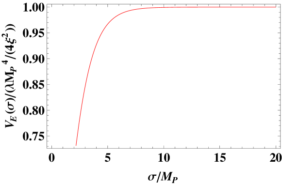
Figure 1: The slow-roll potential needed to drive the cosmological inflation in the Einstein frame.

Then, we quantitatively discuss the cosmological inflation in this extended model. The detailed conditions of the cosmological inflation are described by the following slow-roll parameters:

$$\epsilon =\frac{M_{P}^{2}}{2}\left(\frac{dV_{E}/d{\sigma}}{V_{E}}\right)^{2}=\frac{M_{P}^{2}}{2}\left(\frac{dV_{E}/dr}{V_{E}}\right)^{2}\left(\frac{d\sigma}{dr}\right)^{-2}=\frac{8M_{P}^{4}}{\left(M_{P}^{2}+\xi(6\xi+1)r^{2}\right)r^{2}},$$ (13)

$$\eta =M_{P}^{2}\frac{d^{2}V_{E}/d{\sigma}^{2}}{V_{E}}=M_{P}^{2}\left(\left(\frac{d^{2}V_{E}/dr^{2}}{V_{E}}\right)^{2}\left(\frac{d\sigma}{dr}\right)^{-2}-\frac{dV_{E}/dr}{V_{E}}\left(\frac{d\sigma}{dr}\right)^{-3}\left(\frac{d^{2}\sigma}{dr^{2}}\right)\right)$$

$$=\frac{4M_{P}^{2}(\xi(12\xi+1)r^{2}M_{P}^{2}+3M_{P}^{4}-2\xi^{2}(6\xi+1)r^{4})}{r^{2}(M_{P}^{2}+\xi(6\xi+1)r^{2})^{2}},$$ (14)

where the chain rule is used. The slow-roll parameters $\epsilon$ and $\eta$ imply the first and second derivatives of the potential in the Einstein frame. From Eq. (13) the field value $r_{e}$ at the end of inflation, defined by $\epsilon=1$, is given by

$$r_{e}=M_{P}\sqrt{\frac{\sqrt{192\xi^{2}+32\xi+1}-1}{2\xi(6\xi+1)}}\,.$$ (15)

The number $N$ of e-foldings Linde (2008) is given by

$$N = \frac{1}{\sqrt{2}M_{P}}\int_{r_{{e}}}^{r_{N}}\frac{d\tilde{r}}{\sqrt{\varepsilon(\tilde{r})}}\left(\frac{d\sigma}{d\tilde{r}}\right)$$ (16)

$$= \frac{3}{4}\left[-\ln\frac{M_{P}^{2}+\xi r_{N}^{2}}{M_{P}^{2}+\xi r_{e}^{2}}+\left(\xi+\frac{1}{6}\right)(r_{N}^{2}-r_{e}^{2})/M_{P}^{2}\right],$$

where $r_{N}$ is the field value at Hubble exit during inflation.

The amplitude of density perturbations in $k$-space is defined by the power spectrum:

$$P_{s}(k)=A_{s}\left(\frac{k}{k^{*}}\right)^{n_{s}-1},$$ (17)

where $A_{s}$ is the scalar amplitude at some “pivot point” $k^{*}$, which is given by

$$A_{s}=\frac{V_{E}}{24\pi^{2}M_{P}^{4}\epsilon}\Bigg{|}_{k^{*}},$$ (18)

which can be measured by astrophysical experiments. As a good approximation, the corresponding scalar spectral index $n_{s}$ is given by

$$n_{s}=1-6\epsilon+2\eta\,,$$ (19)

and the tensor-to-scalar ratio $r^{*}$ at leading order is

$$r^{*}=16\epsilon\,.$$ (20)

We use the recent Planck+WP data $\ln(10^{10}A_{s})=3.089^{+0.024}_{-0.027}$ and $n_{s}=0.9603^{+0.024}_{-0.027}$Ade et al. (2013c) to give the constraints on the cosmological parameters and make best fit with respect to the standard Big Bang cosmological model. From Eq. (18), the relation between $\xi$ and $\lambda$ needed to drive the cosmological inflation is shown in Fig. 2.

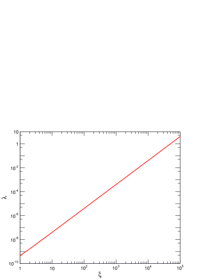
Figure 2: Relation between the nonminimal coupling $\xi$ and self-coupling $\lambda$ needed to drive the cosmological inflation from the data of Planck 2013.

From the Fig. 2, the nonminimal coupling $\xi$ needs to be less than $10^{5}$ if we require the self-coupling $\lambda$ to be less than one because of perturbative theory. Apart from these theoretical arguments, we will discuss the explicit bounds from the experiments of particle physics in the following section. The bound on $n_{s}$ and $r^{*}$ is crucial for constraining the inflationary model. We fit the combined experimental results of Planck and other experimental data using this model as shown in Fig. 3. Since the Planck constraint on $r^{*}$ depends slightly on the pivot scale $k^{*}$, we choose $k^{*}=0.002\rm{Mpc^{-1}}$, and $r_{0.002}^{*}<0.12$ at $95\%$C.L. Figure 3 shows that our prediction is well within the joint $95\%$ C.L. regions for large $\xi$. These results implicate that this model is favored by the astrophysical measurements, which is similar to the $R^{2}$ inflationary model. Compared to other surviving inflationary models after Planck 2013, this model is a concrete realization of these inflationary models and we will discuss the bounds on model parameters from the experiments of the particle physics below.

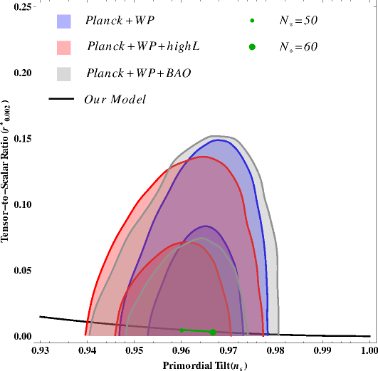
Figure 3: Marginalized joint $68\%$ and $95\%$ C.L. regions for $n_{s}$ and $r^{*}$ from Planck with other data sets compared to the theoretical predictions of this inflationary model for the large $\xi$. ”WP” means the WMAP large-scale polarization. ”BAO” represents the measurements of the baryon acoustic oscillation. ”highL” means large multipole ranges.

III.2 Quantum effects

We now consider the effective potential $V(r)$ or $V_{E}(\sigma)$ at one-loop level, including the effects of the nonminimal coupling of the scalar field $r(x)$ to the gravity $\xi r^{2}R$. The calculation is difficult to perform exactly. However, for large $\xi$, approximate results can be obtained. Under the conformal transformation, the gravity sector becomes canonical, while the kinetic term becomes non-canonical $-{1\over 2}(\partial_{E}r)^{2}(\frac{d}{dr})^{2}$, and we can get a non-standard commutator for $r$ following the approach in Refs. Salopek et al. (1989); De Simone et al. (2009). The canonical momentum corresponding to $r$ is

$$\pi={\partial\mathcal{L}\over\partial\dot{r}}=\sqrt{-g_{E}}\left(g_{E}^{\mu\nu}\,n_{\mu}\,\partial_{\nu}r\right)\left({d\sigma\over dr}\right)^{2}=\sqrt{-g}\left(g^{\mu\nu}\,n_{\mu}\,\partial_{\nu}r\right)f\left({d\sigma\over dr}\right)^{2},$$ (21)

where $n_{\mu}$ is a unit time-like vector. From the standard commutation relation

$$[r({\bf x}),\pi({\bf y})]=i\,\hbar\delta^{(3)}(\bf x-\bf y),$$ (22)

we can obtain

$$[r({\bf x}),\dot{r}({\bf y})]=i\,\hbar\,c_{r}\,\delta^{(3)}({\bf x}-{\bf y}),$$ (23)

with

$$c_{r}={M_{P}^{2}+{\xi r^{2}}\over M_{P}^{2}+(6\xi+1){\xi r^{2}}}.$$ (24)

During inflation, $r\gg M_{P}/\sqrt{\xi}$, there is a suppression factor of $c_{r}=1/(6\xi+1)$ in the commutator. Thus, in the inflationary epoch, quantum loop effects involving the radial boson field $r(x)$ are strongly suppressed. When we calculate the loop corrections, one suppression factor $c_{r}$ is needed for each $r$ propagator in the loop diagram. Using the methods in Ref. Machacek and Vaughn (1983), we can obtain the one-loop running function of the scalar coupling

$$16\pi^{2}\frac{d\xi}{d\ln\mu_{r}/m_{t}}=\frac{2\mathscr{G}}{3}+(6\xi+1)c_{r}\lambda,$$ (25)

where $\mu_{r}$ is the renormalization scale and $m_{t}$ is the top quark mass. Then we calculate the quantum corrections in the Jordan frame. The one-loop correction to the effective potential in the $\overline{MS}$ scheme is given by

$$16\pi^{2}V^{(1)}(r)=A_{r}^{2}\left(\ln{\frac{A_{r}}{\mu_{r}^{2}}}-\frac{3}{2}\right)+\frac{1}{4}B_{r}^{2}\left(\ln{\frac{B_{r}}{\mu_{r}^{2}}}-\frac{3}{2}\right),$$ (26)

where

$$A_{r} = m_{\varphi}^{2}+\frac{1}{2}\mathscr{G}r^{2},$$ (27)

$$B_{r} = -\mu^{2}+3c_{r}\lambda r^{2}.$$ (28)

Finally, we get the effective potential at one-loop level in the Einstein frame:

$$V_{E}=\frac{V^{(1)}+\frac{\lambda}{4}r^{4}}{f^{2}}\,.$$ (29)

IV Constraints from particle physics

In this section we discuss the constraints on the model parameters from the current experimental results in the particle physics. We will investigate whether the experimental data from particle physics can rule out this model. In the following discussions, we will use the relation between $\mathscr{G}$ and $m_{r}$

$$\frac{\mathscr{G}^{2}m_{\mu}^{7}M_{\rm P}}{m_{r}^{4}m_{\varphi}^{4}}\approx 1,$$ (30)

where $m_{\mu}$ is the muon mass. This relation is proposed to explain the fractional cosmic neutrinos Weinberg (2013).

IV.1 SM Higgs invisible decay

Due to the mixing effects between SM Higgs boson and radial field $r^{\prime}$ the invisible decay channel for SM Higgs boson $\varphi^{\prime}\rightarrow\alpha\alpha$ opens. Therefore there exist constraints on the model parameters from the experimental results of Higgs invisible decay, which have been firstly considered in Ref. Weinberg (2013). In our paper based on combined fit results of ATLAS, CMS and Tevatron for the Higgs invisible decay branching ratio Cline et al. (2013), we get the corresponding exclusion region in Fig. 7.

IV.2 Muon anomalous magnetic moment

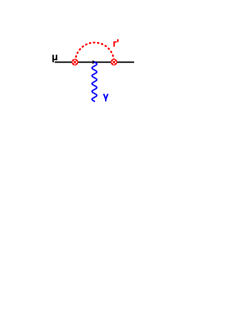
Figure 4: The contribution from the radial boson $r^{\prime}$ to the muon anomalous magnetic moment at the one-loop level.

Through the effective interaction of the radial field with the SM particles, the radial scalar boson $r^{\prime}$ can contribute to the muon anomalous magnetic moment. Up to now there is a $4\sigma$ derivation between SM predictions and experimental results at BNL E821 Teubner et al. (2010):

$$\Delta a_{\mu}=a_{\mu}^{\rm Exp}-a_{\mu}^{\rm SM}=(31.6\pm 7.9)\times 10^{-10}.$$ (31)

At the one-loop level the Feynman diagram of the contribution from the radial boson $r^{\prime}$ to the muon anomalous magnetic moment is shown in Fig 4. After performing perturbative calculations, we can obtain the contribution of $r^{\prime}$ to the muon anomalous magnetic moment

$$\Delta a_{\mu}^{\rm NP}=\vartheta^{2}\frac{G_{\rm F}m_{\mu}^{4}}{4\pi^{2}\sqrt{2}}\int_{0}^{1}\frac{y^{2}(2-y)}{m_{\mu}^{2}y^{2}+m_{r}^{2}(1-y)}dy,$$ (32)

where $G_{\rm F}$ is Fermi constant Beringer et al. (2012). The constraints on the model parameters can be obtained by demanding $\Delta a_{\mu}^{\rm NP}<\Delta a_{\mu}$, and the corresponding exclusion region is shown in Fig. 7.

IV.3 Radiative Upsilon decay $\Upsilon(nS)\rightarrow\gamma+\not{E}$

Figure 5: The Feynman diagram of the contribution from the radial boson $r^{\prime}$ to the process $\Upsilon(nS)\rightarrow\gamma+\not{E}$ at the quark level.

Due to the fact that the main decay channel of $r^{\prime}$ is $r^{\prime}\rightarrow\alpha\alpha$, where $\alpha$ is identified as the missing energy in the experiments, there exist constraints on the model parameter coming from the decay of the meson $\Upsilon(nS)$ into one photon and missing energy. The current experimental results in radiative Upsilon decays $\Upsilon(nS)\rightarrow\gamma+\not{E}$ from BaBar Sekula (2008); Aubert et al. (2008); del Amo Sanchez et al. (2011) are

$$\mathcal{B}r^{\rm BaBar}(\Upsilon(1S)\rightarrow\gamma+\not{E})<2\times 10^{-6},$$ (33)

$$\mathcal{B}r^{\rm BaBar}(\Upsilon(3S)\rightarrow\gamma+\not{E})<3\times 10^{-6}.$$ (34)

In this model at the quark level the Feynman diagram of the contribution from the radial boson $r^{\prime}$ to the process $\Upsilon(nS)\rightarrow\gamma+\not{E}$ is shown in Fig. 5. After performing perturbative calculation we can derive the branching ratio of $\Upsilon(nS)\rightarrow\gamma+r^{\prime}$ at the Born level as

$$\frac{\mathcal{B}r\left(\Upsilon(nS)\rightarrow\gamma+r^{\prime}\right)}{\mathcal{B}r(\Upsilon(nS)\rightarrow\mu^{+}\mu^{-})}=\vartheta^{2}\frac{G_{F}m_{b}^{2}x_{n}}{\sqrt{2}\pi\alpha}\Theta\left(m_{\Upsilon(nS)}-m_{r}\right),$$ (35)

where $m_{\Upsilon(nS)}$ is the mass of $\Upsilon(nS)$ and $\alpha$ is the QED coupling constant. In Eq. 35 the non-perturbative QCD effects have been canceled out in the ratio between $\mathcal{B}r\left(\Upsilon(nS)\rightarrow\gamma+r^{\prime}\right)$ and $\mathcal{B}r(\Upsilon(nS)\rightarrow\mu^{+}\mu^{-})$. After considering the NLO QCD corrections, the branching ratio is given by

$$\frac{\mathcal{B}r\left(\Upsilon(nS)\rightarrow\gamma+r^{\prime}\right)}{\mathcal{B}r(\Upsilon(nS)\rightarrow\mu^{+}\mu^{-})}=\vartheta^{2}\frac{G_{F}m_{b}^{2}x_{n}}{\sqrt{2}\pi\alpha}\left[1-\frac{4\alpha_{s}}{3\pi}f(x_{n})\right]\Theta\left(m_{\Upsilon(nS)}-m_{r}\right),$$ (36)

where $x_{n}=1-m_{r}^{2}/m_{\Upsilon(nS)}^{2}$ and $\alpha_{s}$ is the QCD coupling constants at the scale of $m_{\Upsilon(nS)}$. The function $f(x)$ includes one-loop QCD corrections Nason (1986). Using the above results of BaBar, the corresponding exclusion region can be obtained as shown in Fig. 7.

IV.4 $B$-meson decay $B\rightarrow K+\not{E}$

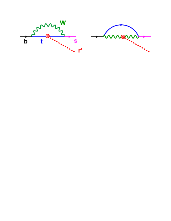
Figure 6: The Feynman diagram of the contribution from the radial boson $r^{\prime}$ to the flavor changing process $B\rightarrow K+\not{E}$ at the quark level.

Now we look at the flavor changing process $B\rightarrow K+\not{E}$. In the SM, for the process of $B$-meson decaying to kaon and a pair of neutrinos, the branching ratio $\mathcal{B}r^{\rm SM}(B\rightarrow K+\nu\bar{\nu})\sim 4\times 10^{-6}$. The present experimental results for $B\rightarrow K+\not{E}$ from CLEO Ammar et al. (2001) and BaBar Aubert et al. (2003); Cartaro (2004) are

$$\mathcal{B}r^{\rm CLEO}(B^{0}\rightarrow K_{s}^{0}+\not{E})<5.3\times 10^{-5},$$ (37)

$$\mathcal{B}r^{\rm BaBar}(B^{-}\rightarrow K^{-}+\not{E})<7.0\times 10^{-5}.$$ (38)

In this model the flavor changing process $B\rightarrow K+r^{\prime}$ is induced at the loop level, and at the quark level the corresponding Feynman diagram is shown in Fig. 6. The low energy effective Lagrangian describing the interaction between $r^{\prime}$, $b$ and $s$ quark can be written as

$$\mathcal{L}_{bsr^{\prime}}=\frac{3g_{w}^{2}m_{b}m_{t}^{2}V_{ts}^{\ast}V_{tb}\vartheta}{64\pi^{2}m_{W}^{2}v}\bar{s}_{L}b_{R}r^{\prime}+{\rm h.c.},$$ (39)

where $g_{W}$ is the weak coupling constant and $v$ is the SM vacuum expectation value. After performing perturbative calculations based on the effective Lagrangian $\mathcal{L}_{bsr^{\prime}}$ and also considering the non-perturbative QCD effects by means of the hadronic form factor determined via light cone sum rule analysis Ali et al. (2000), we get the branching ratio for the process $B\rightarrow K+r^{\prime}$

$$\mathrm{Br}\left(B\rightarrow K+r^{\prime}\right) = \frac{9\sqrt{2}\tau_{B}G_{F}^{3}m_{t}^{4}m_{b}^{2}m_{+}^{2}m_{-}^{2}}{1024\pi^{5}m_{B}^{3}\left(m_{b}-m_{s}\right)^{2}}\left|V_{tb}V_{ts}^{\ast}\right|^{2}f_{0}^{2}\left(m_{r}^{2}\right)$$ (40)

$$\times\sqrt{\left(m_{+}^{2}-m_{r}^{2}\right)\left(m_{-}^{2}-m_{r}^{2}\right)}\;\vartheta^{2}\;\Theta\left(m_{-}-m_{r}\right).$$

Here $m_{\pm}=m_{B}\pm m_{K}$, $m_{B}$ is the mass of $B$-meson, $\tau_{B}$ is the lifetime of $B$ meson, and $V_{tb}$ and $V_{ts}$ are CKM matrix elements. The hadronic form factor $f_{0}\left(x\right)$ is given by  Ali et al. (2000)

$$f_{0}\left(x\right)=0.33\exp\left[\frac{0.63x}{m_{B}^{2}}-\frac{0.095x^{2}}{m_{B}^{4}}+\frac{0.591x^{3}}{m_{B}^{6}}\right].$$ (41)

Using the CLEO experimental results, we obtain the corresponding exclusion region in Fig. 7.

IV.5 Kaon decay $K\rightarrow\pi+\not{E}$

Similar to the case of $B$-meson decay, for the $r^{\prime}$ production through kaon decay $K\rightarrow\pi+\not{E}$, the SM predictions are $\mathcal{B}r^{\rm SM}(K^{+}\rightarrow\pi^{+}+\nu\bar{\nu})=7.8\times 10^{-11}$ Brod et al. (2011). The current experiments’ constraints from E787 and E949 Adler et al. (2002, 2004); Artamonov et al. (2009) are

$$\mathcal{B}r(K^{+}\rightarrow\pi^{+}+\not{E})<10^{-10}.$$ (42)

Using the above experimental results, the corresponding exclusion region can be obtained as shown in Fig. 7.

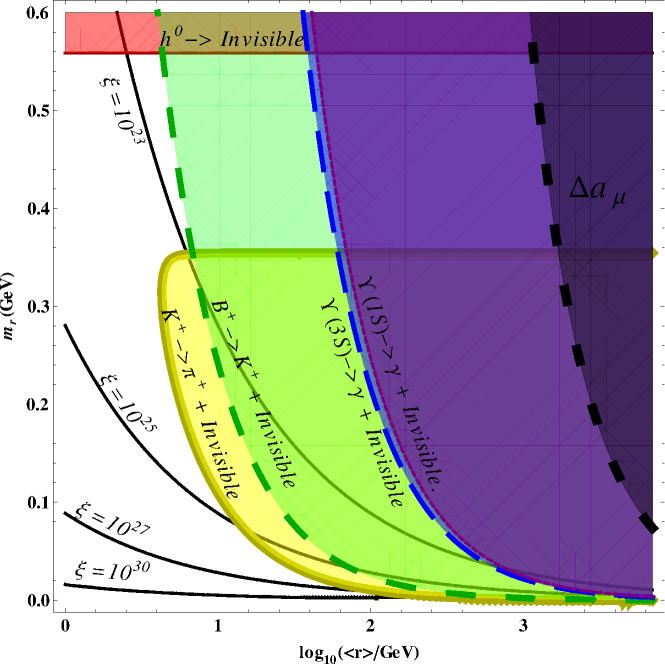
Figure 7: Constraints on the model parameters from Higgs decay, meson decay, and muon anomalous magnetic moment. The colored regions are excluded. Each black line corresponds to the upper bound of $\xi$ for a given mixing angle $\vartheta$($Here,\kappa=3.9\times 10^{15}$).

IV.6 SM Higgs global signal strength

It is important to discuss the dimensionless nonminimal coupling $\xi$ by experiments and test the scalar-tensor interaction Atkins and Calmet (2013); Xianyu et al. (2013) since the effective operator $\xi r^{2}R$ often appears in the quantum gravity theory Chernikov and Tagirov (1968); Callan et al. (1970). In some cases, this nonminimal coupling $\xi$ could be quite large Atkins and Calmet (2013); Xianyu et al. (2013). In this model, we try to give the possible constraints of the nonminimal coupling $\xi$ from the global signal strength of Higgs boson at the LHC.

From the mixing term of radial scalar boson and the Higgs boson, an effective interaction between the Higgs field and the gravitational field can be induced, which is

$$\kappa\varphi^{\dagger}\varphi R,$$ (43)

with

$$\kappa\approx\xi\vartheta^{2}.$$ (44)

We use the recent Higgs data at the LHC and the method in Ref. Atkins and Calmet (2013) to discuss the constraints on the nonminimal coupling of the scalar field to gravity. The relevant action for the Higgs sector is

$$S_{\rm Higgs}=\int d^{4}x\sqrt{-g}\left[\frac{M_{P}^{2}+\kappa\varphi^{\dagger}\varphi}{2}R-\frac{1}{2}\partial_{\mu}\varphi^{\dagger}\partial^{\mu}\varphi\right].$$ (45)

After performing the conformal transformation Salopek et al. (1989)

$$g_{\mu\nu}\to\tilde{g}_{\mu\nu}=\Omega^{2}g_{\mu\nu}\,,\qquad\Omega^{2}=1+\kappa\varphi^{\dagger}\varphi/M_{P}^{2}\,,$$ (46)

the action in the Einstein frame becomes

$$S_{\rm Higgs}^{E}=\int d^{4}x\sqrt{-\tilde{g}}\left[\frac{M_{P}^{2}}{2}\tilde{R}-\frac{3\kappa^{2}}{4M_{P}^{2}\Omega^{4}}\partial_{\mu}(\varphi^{\dagger}\varphi)\partial^{\mu}(\varphi^{\dagger}\varphi)-\frac{1}{2\Omega^{2}}\partial_{\mu}\varphi^{\dagger}\partial^{\mu}\varphi\right],$$ (47)

where the second term comes from the above conformal transformation of the Ricci scalar $R$ Salopek et al. (1989). In this frame, the gravitational sector is of the canonical form, but the kinetic term of the Higgs boson still needs to be cast into the canonical form. After expanding the Higgs field in the unitary gauge and expanding $\Omega^{2}$ at leading order, the kinetic term for the Higgs boson is given by

$$\mathcal{L}_{\rm Higgs}^{\rm kin}=\frac{1}{2}\rho^{2}\frac{\partial_{\mu}\varphi^{\prime}\partial^{\mu}\varphi^{\prime}}{2},$$ (48)

with

$$\rho^{2}=\frac{1}{\Omega_{0}^{2}}+\frac{6\kappa^{2}\langle\varphi\rangle^{2}}{M_{P}^{2}\Omega_{0}^{4}},$$ (49)

where

$$\Omega_{0}^{2}=\frac{M_{P}^{2}+\kappa\langle\varphi\rangle^{2}}{M_{P}^{2}}.$$ (50)

In order to get the canonical kinetic term, all the Higgs couplings to the SM particles should be scaled by $1/\rho$. This leads to a suppression factor of $1/\rho$ for the Higgs boson production and decay at the LHC. By means of the narrow width approximation, we can obtain the global signal strength $\mu_{s}=\sigma/\sigma_{SM}=1/\rho^{2}$. Thus, after considering the best-fit signal strength $\mu_{s}=0.80\pm 0.14$ from CMS CMS (2013) for all channels combined, $\kappa>3.9\times 10^{15}$ is excluded at $95\%$ C.L. This upper bound ($\kappa_{upper}=3.9\times 10^{15}$) is the same order as considered in Ref. Atkins and Calmet (2013). The allowed value for $\kappa$ from Higgs global signal strength is $\kappa<3.9\times 10^{15}$.

IV.7 Discussions

For this inflationary model, the current cosmological experimental data can only give the relation of the nonminimal coupling $\xi$ and the quartic coupling $\lambda$ as shown in Fig. 2. Other considerations come from the theoretic arguments that the quartic coupling should lie in the perturbative regime and the unitarity cutoff should be larger than the involved mass scale of the model. As is shown in Fig. 2, if $\lambda$ is chosen in the perturbative regime, then $\xi<4.7\times 10^{4}$. The unitarity validity needs that the unitarity cutoff $M_{P}/\xi$ should be larger than $m_{r}$. So we will see whether the constraints from the experimental data of particle physics are consistent with the theoretical arguments in the following discussions.

From Eq.(44), for $\xi=\kappa/\vartheta^{2}$, the allowed $\vartheta$ is a function of $m_{r}$ and $\langle r\rangle$ by Eq.(7) (numerically, $\vartheta=\langle r\rangle m_{r}^{2}\times 2.5\times 10^{-4}~{}GeV^{-3}$) and is greatly constrained by the low energy data as shown in Fig. 7, where the colored regions are excluded by the low energy experiments. Figure 8 gives the constraints on the model parameters, $\vartheta$ and $\xi$. The axes of $\vartheta$ and $\kappa$ represent the allowed value of $\vartheta$ from the low energy experiment data($\vartheta<3.3\times 10^{-4}$) and the allowed value of $\kappa$ from the Higgs global signal strength($\kappa<3.9\times 10^{15}$), respectively. The axis of $\xi$ represents the nonminimal coupling $\xi$, and the corresponding $\xi$ values to the points on the green surface are allowed from the experimental data of particle physics. From Fig. 8, we see that $\xi$ covers a wide range of values; especially $\xi$ can take values less than $\xi<4.7\times 10^{4}$, mentioned above. When we fix the value of $\vartheta$, the allowed value for $\xi$ is $\xi<\kappa_{upper}/\vartheta_{allow}^{2}$ for each $\vartheta$. Namely, the upper bound of $\xi$ for each $\vartheta$ is $\xi_{upper}=\kappa_{upper}/\vartheta_{allow}^{2}$. If we take the typical mixing angle $\vartheta=10^{-5}$ ($\vartheta=2\times 10^{-4}$) and the maximal $\kappa$, the corresponding upper bound is $\xi_{upper}=3.9\times 10^{25}$ ($\xi_{upper}=0.925\times 10^{23}$). Compared to the large upper bound of the nonmimal coupling in Ref. Atkins and Calmet (2013), here the larger value of $\xi$ comes from the small mixing angle $\vartheta$ through Higgs portal effects, while $\kappa$ plays the same role as one in Ref. Atkins and Calmet (2013), and their upper bounds are of the same order. In fact, in this scenario considered here $\xi=\kappa/\vartheta^{2}$, and the $\vartheta$ is much smaller than $1$($\vartheta<3.3\times 10^{-4}$), so the value of $\xi$ is greatly enhanced due to the small mixing angle $\vartheta$. This is why there exists a huge gap between $\xi$ and the nonminimal coupling in Ref. Atkins and Calmet (2013).

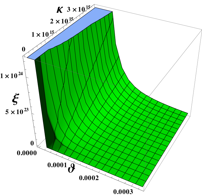
Figure 8: Constraints on the model parameters from low energy data and Higgs data. The axis of $\vartheta$ represents the allowed value of $\vartheta$ from the low energy experiment data($\vartheta<3.3\times 10^{-4}$), the axis of $\kappa$ represents the allowed value of $\kappa$ from the Higgs global signal strength($\kappa<3.9\times 10^{15}$) and the axis of $\xi$ represents the allowed nonminimal coupling $\xi$.

However, if we take a small value of $\kappa$, the value of $\xi$ could be much smaller than the upper bound as shown in Fig. 8, and it can take reasonable values which are consistent with the theoretical arguments. For example, when $\kappa=10^{-4}$ and $\vartheta=10^{-4}$, the corresponding $\xi$ and $\lambda$ are at the order of $10^{4}$ and $0.1$, respectively, which satisfies the inflation condition as shown in Fig. 2 and the constraints from particle physics as shown in Fig. 8. From the theoretical view point, in the above case, the quartic coupling $\lambda<1$ lies in the perturbative regime, and the unitarity violation problem is avoided since $M_{P}/\xi\gg m_{r}$. Therefore, only if the model parameter $\xi$ takes a reasonable value ($\xi<\mathcal{O}(10^{5})$), this inflationary model can simultaneously satisfy theoretical arguments and experimental constraints from particle physics and cosmology.

V Conclusion

We have discussed an extended Higgs portal inflation model, assuming a nonminimal coupling of the scalar field to the gravity. The effective potential which drives cosmological inflation is calculated at both classical and quantum level. Using the new data from Planck and other experiments, we obtain the relation between the nonminimal coupling $\xi$ and the self-coupling $\lambda$ needed to drive the inflation. We find that this inflationary model is favored by the combined results of Planck and other data, since our prediction for $n_{s}$ and $r_{0.002}^{*}$ is well within the region allowed by the current astrophysical measurements. Furthermore, we also give the constraints on the model parameters from the Higgs data at the LHC and the low energy precise data.