Optimal architecture for a non-deterministic noiseless linear amplifier

Abstract

Non-deterministic quantum noiseless linear amplifiers are a new technology with interest in both fundamental understanding and new applications. With a noiseless linear amplifier it is possible to perform tasks such as improving the performance of quantum key distribution and purifying lossy channels. Previous designs for noiseless linear amplifiers involving linear optics and photon counting are non-optimal because they have a probability of success lower than the theoretical bound given by the theory of generalised quantum measurement. This paper develops a theoretical model which reaches this limit. We calculate the fidelity and probability of success of this new model for coherent states and Einstein-Podolsky-Rosen (EPR) entangled states.

A deterministic noiseless, phase insensitive, linear amplifier, as seen in classical systems is unphysical in quantum theory CAV82 . However it has been demonstrated that an analogous probabilistic amplifier is approximately physically realisable ref:Ralph2008 ; ref:Xiang2010 ; ZAV11 and has a wide variety of potential uses in quantum computing and communication technology protocols. These protocols include error correction ref:Ralph2011 , quantum key distribution ref:Blandino2012 and other protocols where distillation of entanglement is desirable ref:Xiang2010 .

In order to translate these systems to useful quantum technologies an investigation into the optimal probabilities of success that can be achieved is important. Low probabilities of success reduce the range of possible experimental and commercial applications of these devices. Ralph and Lund ref:Ralph2008 proposed a linear optics implementation of a heralded noiseless linear amplifier which has been theoretically investigated FIU09 ; GAG12 ; ref:Walk2013 and experimentally demonstrated with good agreement in visibility and effective gain for small amplitudes $\alpha<0.04$ and gains $|g|^{2}\leq 5$ ref:Xiang2010 ; ref:Ferreyrol2008 ; MIC12 ; OSO12 ; KOS13 . The probability of success for low amplitude inputs $\alpha\ll 1$ using this design is $P=\frac{1}{g^{2}+1}$. The probability of success of other linear optical designs are similar ZAV11 ; KIM12 . For higher amplitudes, $\bar{n}$, the probability scales as $P\approx\frac{1}{(g^{2}+1)^{N}}$ where $N\gg|\alpha|^{2}$. The theoretical maximum probability of success for a noiseless linear amplifier in the low photon number regime is $P=\frac{1}{g^{2}}~{}$ref:Ralph2008 and is expected to scale as $\frac{1}{g^{2N}}$.

Our aim in this paper is to identify and analyse a physical model for noiseless linear amplification which saturates this maximum probability of success. Our approach is related to the idea that noiseless amplification can be implemented via a weak measurement model ref:Menzies2009 . The paper is arranged in the following way. In the first section we will introduce a measurement model for noiseless amplification. In section 2 we will translate this into a physical model for the amplifier and particularly look at the low photon number limit. The following two sections will analyse the performance of the amplifier with respect to coherent state inputs and the distillation and purification of Einstein, Podolsky, Rosen (EPR) entanglement (2-mode squeezing). In the final section we will conclude.

I Noiseless amplification as a general measurement

An ideal noiseless amplifier performs the operation $g^{a^{\dagger}a}$ ref:Ralph2008 , that is it takes an input state $\left|\psi\right\rangle$ to $g^{a^{\dagger}a}\left|\psi\right\rangle$. This operator takes the coherent state $\left|\alpha\right\rangle$ to the coherent state $\left|g\alpha\right\rangle$ and is inherently not unitary. This suggests that a measurement process with post-selection on the measurement outcomes is required to implement it. The case we are most interested in here is where $g>1$. In this situation the operator is unbounded and can only be implemented perfectly over the entire Hilbert space via a measurement process with probability zero. In many experimental situations the action of this operator on states with high occupation number are not important as they have negligible amplitude. Therefore this operator is generally chosen to be truncated at some occupation number $N$, which will be chosen depending on the desired performance of an experimental apparatus. This truncation allows for non-zero probabilities of successfully implementing the desired amplification transformation. Lower values of $N$ will generally result in higher probabilities of success at the cost of a lower fidelity of operation when compared to the ideal operation. In current experiments with low energy inputs $N=1$ is sufficient to achieve high fidelity, and this very simple case has non-trivial implications.

When constructing a measurement which implements the amplification, it suffices to consider the case where there is only two outcomes, a success outcome and a failure outcome. When a success outcome is achieved the state is transformed in the required way. Measurement outcomes, which we will label $i$ are represented by $S$ for success and $F$ for failure. The action on the input state due to each measurement result can be represented by the generally non-unitary operator $\hat{M}_{i}$ called the measurement operator. The probability of success for this measurement outcome when the measurement is applied to the state $\left|\psi\right\rangle$ is given by

$$P_{i}=\left\langle\psi\right|\hat{M}_{i}^{\dagger}\hat{M}_{i}\left|\psi\right\rangle$$ (1)

and the resultant output state having achieved the result $i$ is

$$\left|\psi^{{}^{\prime}}_{i}\right\rangle=\frac{\hat{M}_{i}\left|\psi\right\rangle}{\sqrt{P_{i}}}.$$ (2)

To ensure that these operators define a probability measure the condition

$$\hat{M}_{S}\hat{M}^{\dagger}_{S}+\hat{M}_{F}\hat{M}^{\dagger}_{F}=\hat{I}$$ (3)

must be satisfied ref:MikeandIke .

To implement the amplification we require $\hat{M}_{S}\propto g^{a^{\dagger}a}$. To ensure (3) holds over the entire Hilbert space it would be necessary for $\hat{M}_{S}=0g^{\hat{a}^{\dagger}\hat{a}}$ as the eigenvalues of $g^{\hat{n}}$ are unbounded for $g>1$ and $\hat{M}_{F}\hat{M}_{F}^{\dagger}$ must be a positive operator. Now we can make the truncation of this operator to achieve a non-zero probability. We do this by requiring the action on the first $N$ Fock states to be proportional to the those same elements for the perfect amplification operator and leaving the action on higher occupation number states arbitrary. In this case the success measurement operator can be written as

$$\hat{M}_{S}=\mathcal{N}\sum_{n=0}^{N}g^{n}\left|n\right\rangle\left\langle n\right|+\sum_{n=N+1}^{\infty}S_{n}\left|n\right\rangle\left\langle n\right|,$$ (4)

where $S_{n}$ is a sequence of complex numbers with norm between zero and one. This will then allow the operation to satisfy (3) with $\mathcal{N}$ playing the role of the proportionality constant and will in general be non-zero. The probability of success for an arbitrary input state $\left|\psi\right\rangle$ is

$$P_{S}=\left\langle\psi\right|M_{S}^{\dagger}M_{S}\left|\psi\right\rangle=\left|\mathcal{N}\right|^{2}\sum_{n=0}^{N}g^{2n}\left|\left\langle n|\psi\right\rangle\right|^{2}+\sum_{n=N+1}^{\infty}\left|S_{n}\right|^{2}\left|\left\langle n|\psi\right\rangle\right|^{2}.$$ (5)

To ensure that $0\leq P_{S}\leq 1$ for all possible input states $\mathcal{N}\leq g^{-N}$. Here we can see that any complex phase factor within each $S_{n}$ will not influence the probability of success. The fidelity of the success operation for pure state inputs is

$$\mathcal{F}=\frac{\left|\left\langle\psi\right|g^{a^{\dagger}a}M_{S}\left|\psi\right\rangle\right|^{2}}{\left\langle\psi\right|M_{S}^{\dagger}M_{S}\left|\psi\right\rangle}=P^{-1}\left|\mathcal{N}\sum_{n=0}^{N}g^{2n}\left|\left\langle n|\psi\right\rangle\right|^{2}+\sum_{n=N+1}^{\infty}S_{n}g^{n}\left|\left\langle n|\psi\right\rangle\right|^{2}\right|^{2}.$$ (6)

Here the complex phase factors of the $S_{n}$ are important. However if the $S_{n}$ are not real than this can only act to reduce the fidelity. Therefore, to maximise the fidelity and probability over the widest set of states then requires $\mathcal{N}=g^{-N}$ and $S_{n}=1$. This optimised measurement operator is then

$$\hat{M}_{S}=g^{-N}\sum_{n=0}^{N}g^{n}\left|n\right\rangle\left\langle n\right|+\sum_{n=N+1}^{\infty}\left|n\right\rangle\left\langle n\right|$$ (7)

II Measurement model for noiseless amplification

We can construct a model for the generalised measurement described in Eq. 7 by considering a measurement apparatus consisting of a two level system which interacts with the bosonic input mode as shown in Figure 1.

Figure 1: A bosonic system (labeled “System”) interacts with a two-level apparatus (labeled “Apparatus”). The apparatus is prepared into a $Z$ axis spin eigenstate. The interaction applies a conditional unitary rotation where the conditioning depends on the number of bosons in the input. The apparatus is measured and if the spin has flipped then a success is heralded.

After the interaction the apparatus is measured using a projective measurement scheme. The apparatus orthonormal basis states represent success and failure and will be written as $\left|S\right\rangle$ and $\left|F\right\rangle$ respectively. This basis is arbitrary, but the interaction will depend on the particular choice of basis. We will assume that the apparatus is prepared in the $\left|F\right\rangle$ state before the interaction. The interaction is given by the unitary operator

$$\hat{U}=\hat{M}_{S}\otimes\left|S\right\rangle\left\langle F\right|+\hat{M}_{F}\otimes\left|F\right\rangle\left\langle F\right|+\hat{B}_{1}\otimes\left|F\right\rangle\left\langle S\right|+\hat{B}_{2}\otimes\left|S\right\rangle\left\langle S\right|$$ (8)

where $\hat{M}_{S}$ is the operator which will be applied to the system input state when a success result is measured and $\hat{M}_{F}$ is the operator applied to the system on measuring the failure result. The particular form of the operators $\hat{B}_{1,2}$ are not of concern as they are dependent on the apparatus being initialised in the $\left|S\right\rangle$ state. They are included to include enough freedom to ensure that $\hat{U}$ remains unitary. Using the Kronecker product representation of the tensor product the unitarity requirement can be written as

$$\left(\begin{matrix}\hat{M}^{\dagger}_{F}&\hat{M}^{\dagger}_{S}\\ \hat{B}^{\dagger}_{1}&\hat{B}^{\dagger}_{2}\end{matrix}\right)\left(\begin{matrix}\hat{M}_{F}&\hat{B}_{1}\\ \hat{M}_{S}&\hat{B}_{2}\end{matrix}\right)=\left(\begin{matrix}\hat{I}&0\\ 0&\hat{I}\end{matrix}\right)$$ (9)

which can be rewritten as

$$\hat{M}_{F}^{\dagger}\hat{M}_{F}+\hat{M}_{S}^{\dagger}\hat{M}_{S} = \hat{I}$$ (10)

$$\hat{M}_{F}^{\dagger}\hat{B}_{1}+\hat{M}_{S}^{\dagger}\hat{B}_{2} = 0$$ (11)

$$\hat{B}_{1}^{\dagger}\hat{B}_{1}+\hat{B}_{2}^{\dagger}\hat{B}_{2} = \hat{I}$$ (12)

Provided $\hat{M}_{S}$ and $\hat{M}_{F}$ define a set of measurement operators (in particular the requirement in equation (3)) then the first and last equations are always satisfied if $\hat{B}_{1}=\pm\hat{M}_{S}$ and $\hat{B}_{2}=\pm\hat{M}_{F}$. The second equation could never be satisfied had we swapped the success and failure operators in this assignment. If $\hat{M}_{S}$ and $\hat{M}_{F}$ are Hermitian and commute, as is the case we are considering here, then we can always satisfy the second equation by choosing $\hat{B}_{1}=-\hat{M}_{S}$ and $\hat{B_{2}}=\hat{M}_{F}$.

Now we can substitute our success operator from equation (7) into this interaction unitary. This unitary can then be rearranged to be written as

$$\hat{U}=\sum_{n=0}^{\infty}\left|n\right\rangle\left\langle n\right|\otimes\hat{R}_{n}$$ (13)

where $\hat{R}_{n}$ is defined as

$$\hat{R}_{n}=\left(\begin{matrix}\sqrt{1-G_{n}^{2}}&G_{n}\\ -G_{n}&\sqrt{1-G_{n}^{2}}\end{matrix}\right),$$ (14)

$$G_{n}=\min(1,g^{(n-N)}).$$ (15)

The operator $\hat{R}_{n}$ is a Pauli Y-rotation of $\theta=2\arcsin\left(\min(1,g^{n-N})\right)$ on the heralding qubit which depends on the number of bosons in the input mode. This unitary can be generated by the Hamiltonian

$$\hat{H} = \frac{\hbar}{\tau}\left[\sum_{n=0}^{\infty}\arcsin(\min(1,g^{n-N}))\hat{Y}\otimes\left|n\right\rangle\left\langle n\right|\right]$$ (16)

$$= \frac{\hbar}{\tau}\arcsin(\min(1,g^{\hat{a}^{\dagger}\hat{a}-N}))\otimes\hat{Y},$$

where $\tau$ is the interaction time which is chosen to ensure the apropriate that the rotation parameter $\theta$ is implemented.

II.1 Low photon number limit

In the limit of low amplitude inputs we can implement the amplifier with $N=1$. The system can then be considered a qubit and the gate between the system and the apparatus is locally equivalent to a standard controlled rotation. To see this, we take the unitary from equation 13

$$\hat{U}_{N=1}=\left|0\right\rangle\left\langle 0\right|\otimes\left(\begin{matrix}\sqrt{1-1/g^{2}}&1/g\\ -1/g&\sqrt{1-1/g^{2}}\end{matrix}\right)+\left|1\right\rangle\left\langle 1\right|\otimes\left(\begin{matrix}0&1\\ -1&0\end{matrix}\right)$$ (17)

and then decompose it into

$$\hat{U}_{N=1}=-(X\otimes X)(I\otimes Z)C(R_{y}(\theta))(X\otimes I)$$ (18)

where $X$ and $Z$ are the standard Pauli matricies and $C(R_{y}(\theta))$ is a controlled Pauli $Y$ rotation by $\theta$ and $\theta$ is as defined above with $n=0$ and $N=1$. Applying this unitary to states of the form $\left|0\right\rangle+\alpha\left|1\right\rangle$ where $\alpha$ is small results in the probability of success for the noiseless amplification of $\frac{1}{g^{2}}$.

III Coherent state inputs

We can now calculate the performance of this model for particular situations. First we will calculate the action on coherent states. Coherent states are an ideal test of the amplification process as the expected output from the amplification is easy to define. The ideal amplification action on a coherent state is

$$g^{a^{\dagger}a}\left|\alpha\right\rangle=e^{(g^{2}-1)|\alpha|^{2}/2}\left|g\alpha\right\rangle.$$ (19)

This can then be used to calculate the probability of success and the fidelity of our model amplifier for coherent state inputs denoted by $P_{c}$ and $\mathcal{F}_{c}$ respectively,

$$P_{c}=\left\langle\alpha\right|M_{S}^{\dagger}M_{S}\left|\alpha\right\rangle=e^{-\left|\alpha\right|^{2}}\left[g^{-2N}\sum_{n=0}^{N}g^{2n}\frac{\left|\alpha\right|^{2n}}{n!}+\sum_{n=N+1}^{\infty}\frac{\left|\alpha\right|^{2n}}{n!}\right],$$ (20)

$$\mathcal{F}_{c}=P_{c}^{-1}\left|\left\langle g\alpha\right|M_{s}\left|\alpha\right\rangle\right|^{2}=P_{c}^{-1}e^{-(1+g^{2})\left|\alpha\right|^{2}}\left|g^{-N}\sum_{n=0}^{N}g^{2n}\frac{\left|\alpha\right|^{2n}}{n!}+\sum_{n=N+1}^{\infty}g^{n}\frac{\left|\alpha\right|^{2n}}{n!}\right|^{2}.$$ (21)

These expressions can be written in terms of incomplete gamma functions

$$P_{c}=P(N+1,|\alpha|^{2})+g^{-2N}e^{(g^{2}-1)|\alpha|^{2}}Q(N+1,|g\alpha|^{2}),$$ (22)

$$F_{c}=P_{c}^{-1}e^{-(1+g^{2})|\alpha|^{2}}\left|g^{-N}e^{|g\alpha|^{2}}P(N+1,|g\alpha|^{2})+e^{g|\alpha|^{2}}Q(N+1,g|\alpha|^{2})\right|^{2}$$ (23)

where $Q(N,\lambda)$ is the regularlised incomplete gamma function defined as

$$Q(N,\lambda)=\Gamma(N,\lambda)/\Gamma(N)$$ (24)

where $\Gamma(N,\lambda)$ is the incomplete gamma function, $\Gamma(N)$ is the complete gamma function and $P(N,\lambda)=1-Q(N,\lambda)$ gammafunc . The appearance of the incomplete gamma functions here is expected as this function is the cumulative distribution function for the Possionian distribution which is the distribution that would result when measuring a coherent state in the Fock basis. In this form these equations can be rapidly computed numerically for particular values of $g$, $\alpha$ and $N$. Figure 2 shows $P_{c}$ and $F_{c}$ for $\alpha=0.8$ and $N=1,2,3$ and $4$.

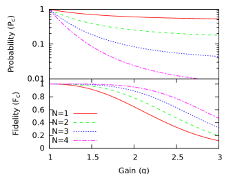
Figure 2: Probability of success and fidelity for an input coherent state with amplitude $\alpha=0.8$ for $N=1,2,3$ and $4$. These curves are calculated from equations 22 and 23.

The probability drops away from $1$ for small gains and the rate at which this occurs increases as $N$ increases. The fidelity initially stays close to $1$ for small amplitudes but eventually drops and the gain at which this occurs increases as $N$ increases. Whilst these properties are evident in the figure, they are general features given that $\alpha$ is fixed.

Low fidelity operation is not of great interest for building a device which performs linear amplification. Therefore we will set a bound on performance that is deemed acceptable. Quantitatively we will require a minimum fidelity $\mathcal{F}\geq 0.99$. The fidelity will increase towards $1$ as $N$ increases hence in any particular situation we can choose an $N$ to achieve this fidelity requirement. Figure 3 shows the effect of enforcing this minimum acceptable fidelity.

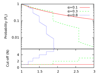
Figure 3: Probability of success for coherent state inputs with amplitude $\alpha=0.1,0.3,0.8$ for gains between $g=1$ and $4$. Cut-off $N$ is chosen to ensure an output fidelity more than $0.99$. Discontinuous jumps occur when the fidelity bound is reached and the value of $N$ is incremented. The corresponding values for $N$ are shown in the lower plot.

The most notable effect that can be seen is the discontinuous jumps in the probability of success. A jump occurs when the cut-off $N$ is incremented to enforce the minimum fidelity. This means that the probability of success is made up of pieces from the probabilities like what is shown in figure 2 for $\alpha=0.8$. Also of note, is that for low amplitude inputs (here $\alpha=0.1$) then choosing $N=1$ provides an acceptable reproduction of linear amplification over a wide range of gain (here $1\leq g\leq 3$).

IV EPR state inputs

An important application of this type of amplification is distilling continuous variable entanglement ref:Xiang2010 ; ref:Blandino2012 . The action of the amplifier is easiest to calculate for an ideal Einstein-Podolsky-Rosen (EPR) state

$$\left|EPR\right\rangle=\sqrt{1-\chi^{2}}\sum_{n=0}^{\infty}\chi^{n}\left|n,n\right\rangle,$$ (25)

where the parameter $0\leq\chi<1$ is representative of the strength of the continuous variable entanglement. The ideal amplification of this state is then

$$g^{a^{\dagger}a}\left|EPR\right\rangle\propto\sum_{n=0}^{\infty}(g\chi)^{n}\left|n,n\right\rangle.$$ (26)

The action of the amplifier preserves the form of the EPR state but increases the entanglement. Note that this places an upper bound on $g$. For if $g>1/\chi$ then the coefficients in the summation diverge. What this means is that when an implementation chooses an $N$ cut-off, the output state does not converge towards a particular state in the limit as $N\rightarrow\infty$. This phenomenon will also found when applying ideal amplification to a distribution of coherent states which forms a mixed state ref:Walk2013 .

The EPR state can be generalised to include losses. Here we will concentrate on the case where only one of the EPR modes undergoes loss of amplitude $\eta$. The state from this is a three mode state

$$\frac{\left|EPR_{l}\right\rangle}{\sqrt{1-\chi^{2}}}=\sum_{n=0}^{\infty}\sum_{t=0}^{n}\chi^{n}\sqrt{\binom{n}{t}\eta^{t}\left(1-\eta\right)^{n-t}}\left|n,t,n-t\right\rangle$$ (27)

where the third mode represents the loss mode which is assumed to be inaccessible to any experiment.

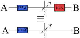
Figure 4: The state generated by an ideal noiseless linear amplifier on a single sided lossy EPR state is another single sided lossy EPR state but with different variables for the strength of the squeezing and loss. The parameters of the state after the amplification $\chi^{\prime}$ and $\eta^{\prime}$ are related to the input state parameters $\chi$ and $\eta$ and the gain of the amplification $g$ (equations 31, 32 and 33).

As in the case of the pure EPR state, the lossy EPR state under ideal amplification is another lossy EPR state but with different parameters, see figure 4. Applying the ideal amplification to the second mode in equation 27 introduces a $g^{t}$ into the coefficients. Then equating this to another lossy EPR state characterised by squeezing $\chi^{\prime}$ and transmission $\eta^{\prime}$ gives the relations

$$\chi^{n}g^{t}\sqrt{\eta}^{t}\left(\sqrt{1-\eta}\right)^{n-t}={\chi^{\prime}}^{n}\sqrt{\eta^{\prime}}^{t}\left(\sqrt{1-\eta^{\prime}}\right)^{n-t}$$ (28)

which must hold true for all integers $n\geq 0$ and $0\leq t\leq n$. Two separate equations can be obtained from this,

$$\chi\sqrt{1-\eta}=\chi^{\prime}\sqrt{1-\eta^{\prime}}$$ (29)

$$\chi g\sqrt{\eta}=\chi^{\prime}\sqrt{\eta^{\prime}},$$ (30)

which can be inverted to give

$$\chi^{\prime}=f\chi,$$ (31)

$$\eta^{\prime}=\frac{g^{2}}{f^{2}}\eta,$$ (32)

$$f=\sqrt{1-\eta+\eta g^{2}}.$$ (33)

The possibility of non-convergence of the output state, just as seen for pure EPR inputs, is present here as well. Convergence will be achieved provided $\chi^{\prime}<1$.

We will consider $\eta$ to be a fixed value and choose $\chi^{\prime}$ to be a fixed in the sense that some target squeezing strength is desired. In this way we can avoid choosing gains for which the output is not convergent.

We will focus here on the ability of the state to demonstrate the EPR paradox reid1998 ; ou1992 . This is achieved by EPR criterion $\varepsilon_{EPR}<1$ where

$$\varepsilon_{EPR}=V_{B|A}^{+}V_{B|A}^{-}$$ (34)

and $V_{B|A}^{\pm}$ is the conditional variance of the $B$ mode on $A$ and the superscript represents the quadrature in which the variance is calculated. The conditional variance is defined as

$$V_{B|A}^{\pm}=\min_{0\leq g\leq 1}\left<(X_{B}^{\pm}\mp gX_{A}^{\pm})^{2}\right>,$$ (35)

and for the EPR state with one sided loss the optimisation gives bernu

$$V^{+}_{B|A}=V^{-}_{B|A}=1-\frac{2\chi^{2}\eta}{1+\chi^{2}},$$ (36)

and hence the EPR criterion in this case is

$$\varepsilon_{EPR}=\left(1-\frac{2\chi^{2}\eta}{1+\chi^{2}}\right)^{2}.$$ (37)

When the amplifier succeeds, both the effective squeezing and transmission are greater then their initial counterparts. The amplifier has a purifing action on this state. This means that it is possible to reach a lower EPR criterion then would be otherwise possible.

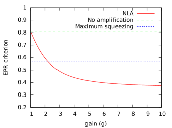
Figure 5: The EPR criterion as a function of gain with a target output squeezing of $\chi^{{}^{\prime}}=0.5$ and an initial transmission of $\eta=0.25$. The red line indicates the initial EPR criterion (no amplification), while the green line represents the maximum EPR criterion that could be obtained by using a squeezed state with $\chi\rightarrow 1$ without making use of a noiseless amplifier.

Figure 5 shows the EPR criterion for an output squeezing of $\chi^{{}^{\prime}}=0.5$ with a channel transmission of $\eta=0.25$. The lowest EPR condition possible without amplification given the channel loss (i.e. $\chi\rightarrow 1$) is achieved by amplifying the lossy EPR state when $g\approx 2.5$.

The state conditional on achieving success is

$$M_{s}\left|EPR_{l}\right\rangle=\sum_{t=0}^{\infty}\sum_{n=t}^{\infty}\mathrm{min}(g^{t-N},1)\chi^{n}\sqrt{\binom{n}{t}\eta^{t}(1-\eta)^{n-t}}\left|n,t,n-t\right\rangle.$$ (38)

The probability of success for our model amplifier on this type of input state can be simply computed as $P_{EPR}=\left\langle EPR\right|\hat{M}_{S}^{\dagger}\hat{M}_{S}\left|EPR\right\rangle$ just as before

$$P_{EPR}=(1-\chi^{2})\left(\frac{g^{-2N}}{1-\chi^{2}(1+(g^{2}-1)\eta)}+\sum_{n=N+1}^{\infty}\chi^{2n}\sum_{t=N+1}^{n}\binom{n}{t}\left(1-g^{2(t-N)}\right)\eta^{t}(1-\eta)^{n-t}\ \right).$$ (39)

A sum can be removed from this equation by using the relationship

$$\sum_{t=N+1}^{n}\binom{n}{t}a^{t}b^{n-t}=(a+b)^{n}I_{\frac{a}{a+b}}(N+1,n-N),$$ (40)

where $I_{x}(a,b)$ is the regularised incomplete beta function betafunc , giving

$$P_{EPR}=(1-\chi^{2})\left(\frac{g^{-2N}}{1-{\chi^{\prime}}^{2}}+\sum_{n=N+1}^{\infty}\left(\chi^{2n}I_{\eta}(N+1,n-N)-g^{-2N}{\chi^{\prime}}^{2n}I_{\eta^{\prime}}(N+1,n-N)\right)\right).$$ (41)

To compute fidelity is more difficult because when the loss mode is traced out the resulting state is mixed. We can calculate a lower bound on the fidelity by computing the fidelity of the amplified state compared to the purified lossy EPR state with squeezing $\chi^{\prime}$ and loss $\eta^{\prime}$, i.e. $\mathcal{F}_{EPR}=P_{EPR}^{-1}\left|\left\langle EPR^{{}^{\prime}}\right|\hat{M}_{S}\left|EPR\right\rangle\right|^{2}$

$$\frac{\sqrt{\mathcal{F}_{EPR}P_{EPR}}}{\sqrt{(1-\chi^{2})(1-\chi^{\prime 2})}}=\frac{g^{-N}}{1-(g\sqrt{\eta\eta^{\prime}}+\sqrt{(1-\eta)(1-\eta^{\prime})})\chi\chi^{\prime}}+\sum_{n=N+1}^{\infty}(\chi\chi^{\prime})^{n}\sum_{t=N+1}^{n}\binom{n}{t}(1-g^{t-N})\sqrt{\eta\eta^{\prime}}^{t}\sqrt{(1-\eta)(1-\eta^{\prime})}^{n-t}$$ (42)

$$\eta_{1}=\sqrt{\eta\eta^{\prime}}+\sqrt{(1-\eta)(1-\eta^{\prime})}=\frac{1-\eta+g\eta}{f}$$ (43)

$$\eta_{2}=g\sqrt{\eta\eta^{\prime}}+\sqrt{(1-\eta)(1-\eta^{\prime})}=f$$ (44)

$$\frac{\sqrt{\mathcal{F}_{EPR}P_{EPR}}}{\sqrt{(1-\chi^{2})(1-\chi^{\prime 2})}}=\frac{g^{-N}}{1-\eta_{2}\chi\chi^{\prime}}+\sum_{n=N+1}^{\infty}(\chi\chi^{\prime})^{n}\left(\eta_{1}^{n}I_{\sqrt{\eta\eta^{\prime}}/\eta_{1}}(N+1,n-N)-g^{-N}\eta_{2}^{n}I_{g\sqrt{\eta\eta^{\prime}}/\eta_{2}}(N+1,n-N)\right)$$ (45)

where $f$ is defined in Equation 33.

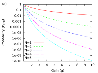
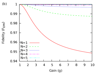
Figure 6: Probability and fidelity for the EPR state characterised by an effective squeezing of $\chi^{\prime}=0.5$ and a transmission of $\eta=0.3$ undergoing amplification with truncation numbers $N=1$ to $N=5$.

The probability and fidelity for $N=1$ to $5$ with $\chi^{\prime}=0.5$ and $\eta=0.3$ are shown in figure 6. The probabilities drop exponentially with gain, but the fidelity drops slowly. This is because as the gain increases a lower $\chi$ is used to ensure that $\chi^{\prime}$ stays fixed. The asymptotic behaviour of these functions as $g\rightarrow\infty$ is

$$P_{EPR}=g^{-2N}\left(\frac{1-{\chi^{\prime}}^{2N+2}}{1-{\chi^{\prime}}^{2}}\right)+O(g^{-2N-1}),$$ (46)

$$\mathcal{F}_{EPR}P_{EPR}=g^{-2N}\frac{(1-{\chi^{\prime}}^{2N+2})^{2}}{1-{\chi^{\prime}}^{2}}+O(g^{-2N-1}).$$ (47)

Hence we find that the fidelity asymptotically approaches a constant value

$$\mathcal{F}_{EPR}=1-{\chi^{\prime}}^{2N+2}+O(g^{-1}).$$ (48)

The fidelity will always be $1$ at $g=1$ and for larger $g$ then approaches this constant value from above. Therefore this number constitutes a lower bound on the fidelity.

As was indicated before in the analysis for coherent state inputs, the low fidelity operation is not usually of interest. When designing an experiment there is usually some minimum fidelity and probability of success that is deemed acceptable. The order of magnitude for these is dependant on the on the experimental conditions. We will now consider these factors to further analyse the action of this model amplifier.

We can use this expression for the limiting case of fidelity to explicly compute a maximum $N$ under restrictions in the fidelity and entanglement. A fidelity minimum is chosen $\mathcal{F}_{min}<1$ and at all times the performance of amplification must always be higher than this number. Also, if there is a maximum $\chi^{\prime}<1$ for which amplifications cannot exceed after successful amplification, then it must be true that

$$N\leq\frac{\log{\left(1-\mathcal{F}_{min}\right)}}{2\log{\chi^{\prime}}}-1$$ (49)

Note that this requirement is independent of the probability of success.

To consider both a probability and fidelity bound we consider a numerical optimisation of the EPR criterion for an amplified EPR state which results a particular output squeezing $\chi^{\prime}$ which has undergone one sided loss $1-\eta$. The optimisation we will consider here enforces a fidelity greater than $0.99$ and the probability of success greater than either $0.1$, $0.01$ and $0.001$. Because of the monotonic nature of the fidelity and probability under such conditions, we find that this optimisation always occurs on the boundary of either the probability constraint or the fidelity constraint. Figure 7 shows the results of this optimisation when $\chi^{\prime}=0.5$ and $0.8$ as a function of loss.

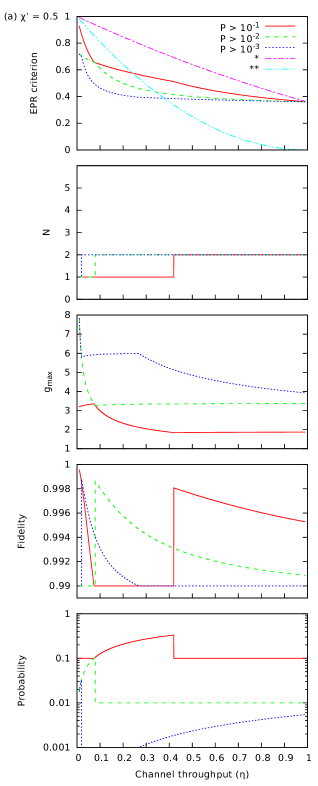
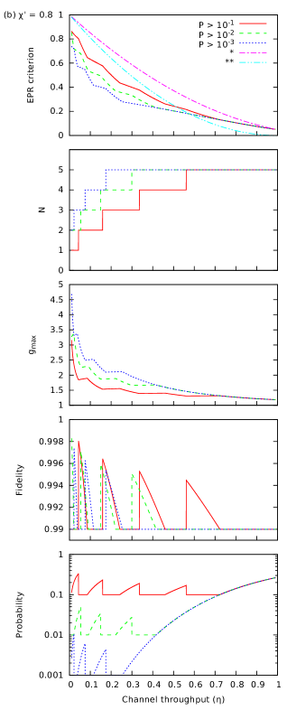
Figure 7: Plots of the lowest possible EPR criterion, $N$, gain $g$, lower bound of fidelity and probability of success which achieve the of lowest possible EPR criterion, $\varepsilon_{EPR}$ such that $\mathcal{F}_{min}>0.99$, probability of success $P>0.1$ (solid line), $0.01$ (dashed line) and $0.001$ (dotted line) and output squeezing of $\chi^{\prime}=0.5$ shown in (a) and $\chi^{\prime}=0.8$ shown in (b). The x-axis of each plot is the channel throughput $\eta$. The plots showing the optimised EPR criterion have curves showing the EPR criterion when no amplification is performed (*, dash-dot line) and the EPR criterion with no amplification with an infinitely squeezed source with the same loss (**, dash-dot-dot line).

The results of this optimisation are best understood by starting at the case where $\eta=1$. For this case we want to find if we are at the boundary of the fidelity or probability constraints whilst ensuring that both constraints are satisfied. Also, the largest possible gain which achieves the fidelity constraint will occur at the lowest value for $N$. Therefore we seek the gain and lowest $N$ such that our fidelity and probability constraints are satisfied. As the loss is increased, less signal is amplified and the fidelity and probability increase. Therefore a larger gain can be chosen which still satisfies the constraints. This continues until such point as the input signal is weak enough so that the next lowest $N$ satisfies the constraints. This results in a discontinuous jump in the output. Also, if the probability was the saturated constraint, when $N$ is decremented this may change to the fidelity constraint being the one that is saturated. As loss is increased further there will be a point where the saturation of these constraints will swap. This results in sharp corners appearing in the maximised curves for the gain and EPR criterion.

The figures also show a comparison of this best EPR criterion to particular situations not involving any amplification process. The amplification process always produces a lower EPR criterion when compared with doing no amplification. However, it is probably of more interest to compare the situation to that of assuming the entanglement source could in principle produce a maximally entangled EPR state (i.e. $\chi=1$). Because of the loss, the EPR criterion for this limiting case is not zero. Our amplification model can succeed in producing a lower EPR criterion than that of the maximally entanged source. As shown in Figure 7 this improvement occurs in high loss situations. The parameters for which this improvement occurs will depend on the value of $\chi^{\prime}$ chosen. But as shown in figure 7 the range of losses for which this occurs can cover a significant range.

V Conclusion

This paper has demonstrated a new model which could be used as a noiseless phase insensitive linear amplifier. We have presented a unitary for the non-conditional evolution of a coupled harmonic oscillator system and a heralding qubit. This evolution can then be used as a probabilistic amplifier by measuring the heralding qubit after the unitary evolution. The evolution is not that of a linear optical transformation, but does achieve the highest theoretically possible probability of success. The action of our noiseless amplification model on a coherent state and an EPR state was computed. For an EPR state undergoing one sided loss, we found that for sufficiently high loss it is possible for the amplifier to achieve an EPR criterion lower than that possible using an unamplified infinite squeezed source passing through the same loss. By choosing our parameters such that we target a particular level of two-mode squeezing when the amplification succeeds, we have shown that, for the case of single sided loss, the fidelity of the amplification has a lower bound. This model and the results we have computed here may be used as a guide to future experiments which wish to operate near the optimal probability of success.

VI Acknowledgements

This research was conducted by the Australian Research Council Centre of Excellence for Quantum Computation and Communication Technology (Project number CE110001027).

References

- (1) C. M. Caves, Phys. Rev. D 26, 1817 (1982).
- (2) T. C. Ralph and A. P. Lund, Quantum Communication Measurement and Computing Proceedings of 9th International Conference p. 155 (2009).
- (3) G. Y. Xiang, T. C. Ralph, A. P. Lund, N. Walk, and G. J. Pryde, Nature Photonics 4, 316 (2010).
- (4) A. Zavatta, J. Fiurás̆ek, and M. Bellini, Nature Photon 5, 52 (2011).
- (5) T. C. Ralph, Physical Review A, 84, 022339 (2011).
- (6) R. Blandino, A. Leverrier, M. Barbieri, J. Etesse, P. Grangier, R. Tualle-Brouri, Phys. Rev. A 86, 012327 (2012).
- (7) F. Ferreyrol, M. Barbieri, R. Blandino, S. Fossier, R. Tualle-Brouri, and P. Grangier, Phys. Rev. Lett. 104, 123603 (2010).
- (8) J. Fiurás̆ek, Physical Review A 80, 053822 (2009).
- (9) C. Gagatsos, E. Karpov, and N. J. Cerf, Phys. Rev. A 86, 012324 (2012).
- (10) N. Walk, A. P. Lund and T. C. Ralph, arXiv:1211.3794.
- (11) M. Micuda, I. Straka, M. Mikova, M. Dusek, N. J. Cerf, J. Fiurás̆ek, M. Jezek, Phys. Rev. Lett. 109, 180503 (2012).
- (12) C. I. Osorio, N. Bruno, N. Sangouard, H. Zbinden, N. Gisin, R. T. Thew, Phys. Rev. A 86, 023815 (2012).
- (13) S. Kosis, G. Y. Xiang, T. C. Ralph and G. J. Pryde, Nature Physics 9, 23 (2013).
- (14) H.-J. Kim, S.-Y. Lee, S.-W. Ji, and H. Nha, Physical Review A 85, 013839 (2012).
- (15) D .Menzies and S .Croke. arXiv:0903.4181.
- (16) F. Ferreyrol, R. Blandino, M. Barbieri, R. Tualle-Brouri, and P. Grangier, Physical Review A 83, 063801 (2011).
- (17) M. A. Nielsen and I. L. Chuang, Quantum computation and quantum information. Cambridge University Press, New York, 2000.
- (18) S. Pandey, Z. Jiang, J. Combes, C. M. Caves, arXiv:1304.3901 (2013).
- (19) M. D. Reid and P. D. Drummond, Phys. Rev. Lett. 60, 2731 (1988).
- (20) Z. Y. Ou, S. F. Pereira, H. J. Kimble, and K. C. Peng, Phys. Rev. Lett. 68, 3663 (1992).
- (21) We have used the definition of the incomplete gamma function as the integral . The and notation we have used for the regularised incomplete gamma functions is widely used but not universally used. See http://mathworld.wolfram.com/RegularizedGammaFunction.html
- (22) We have used the definition of the beta function as and the regularlised beta function is then .
- (23) J. Bernu, private communication (2012).