Flow-level performance of random wireless networks

Richard Combes and Eitan Altman    Richard Combes (1,2), and Eitan Altman (2) 1KTH, Royal Institute of Technology, Stockholm, Sweden 2INRIA Sophia Antipolis, France
Abstract

We study the flow-level performance of random wireless networks. The locations of base stations (BSs) follow a Poisson point process. The number and positions of active users are dynamic. We associate a queue to each BS. The performance and stability of a BS depend on its load. In some cases, the full distribution of the load can be derived. Otherwise we derive formulas for the first and second moments. Networks on the line and on the plane are considered. Our model is generic enough to include features of recent wireless networks such as 4G (LTE) networks. In dense networks, we show that the inter-cell interference power becomes normally distributed, simplifying many computations. Numerical experiments demonstrate that in cases of practical interest, the loads distribution can be well approximated by a gamma distribution with known mean and variance. 111Richard Combes is with KTH. Major parts of this work were done when he was in INRIA.

Index Terms:
Wireless networks, Performance Evaluation, Queuing theory, Traffic models, Flow-level dynamics, Stochastic geometry, Point processes.

I Introduction

The most straightforward approach to performance evaluation of wireless networks is to assume that BS locations are deterministic and follow a regular pattern such as an hexagonal grid on the plane. A more recent trend is to consider random BS locations. Namely BS locations form a stationary point process rather than a deterministic pattern. One of the motivations for this approach is that operational networks are hardly regular, due to irregular city planning, legal constraints on BS placement and non homogeneity of traffic density. When the BS locations follow a PPP (PPP), many performance indicators can be calculated in closed form or with simple numerical integrals, so that this approach is tractable. A summary of both the theory and networking applications can be found in [1, 2].

Another characteristic of wireless network is the dynamic user behavior (also called flow-level dynamics). Users enter the network at random locations and instants to receive a service, and leave after service completion. Users may move during their service. Network resources are shared between active users so that the time spent by different users is not independent i.e there is congestion. Congestion due to dynamic user behavior is modeled by queueing theory: each BS is modeled as a queue, and the system performance is derived from its stationary distribution, providing that the queue is stable. Queuing models for wireless networks serving streaming traffic [3, 4, 5], elastic traffic [6, 7] and a mix of both [8] have been studied in the literature. An important characteristic is the performance of a BS is its load. In particular, without admission control, the number of active users grows without bound if the load is strictly larger than 111.

Related work:

Assuming that users are served by the closest BS, the zones served by BS are Poisson-Voronoi cells. The geometry of Poisson-Voronoi cells is a well studied topic because of its applications to physics and more recently networking. The mean and variance of the cell area is studied in [9]. Statistical studies show that the cell area distribution can be approximated with good accuracy by a gamma distribution [10] or a generalized gamma distribution [11]. [12] investigates the distribution of the smallest disk containing the Voronoi cell which can serve as an upper bound. The number of sides of the cell was studied in [13]. Conditional to the number of faces of the cell, [14] showed that the fundamental area of the cell follows a Gamma distribution and [15] gives the distribution of the cell area. A more general gamma-type result is given in [16]. In [17], the authors consider the distribution of the integral of a function of the distance over the cell, and calculate its first and second moments as well as its tail behavior.

There is a large amount of recent results on the performance evaluation of wireless networks using stochastic geometry. Most works assume that BS locations follow a PPP. Distribution of the covered areas is studied in [18]. The distribution of the SINR (SINR) and data rate in downlink cellular networks is derived in [19]. [20] treats the uplink case. Downlink heterogenous networks are considered in [21, 22, 23, 24, 25], and the different types of BS are assumed to follow independent PPP. User association and fractional frequency reuse are studied in [26] and [24] respectively. The handover probability of a typical user is studied in [27]. Concerning non-Poisson networks, [28] studies the distribution of shot-noise and [29] examines the performance gap between PPP and non-Poisson networks.

All these results concern “single user” performance evaluation and do not take into account dynamic user behavior. Namely, only the distribution of the SINR, data rate etc. for a single user located at the origin are derived. In [30, 21, 22], a random number of users is considered. However, the time a user spends in the network does not depend on his position or on the number of users connected to the same serving BS i.e the congestion is not taken into account. For elastic traffic for instance, the time spent by a user to transmit a given amount of data depends on his throughput which is a function of its position, interference and congestion. Furthermore [30, 21] approximate the cell size distribution by a gamma distribution, as proposed by [10, 11].

Our contribution:

In this paper, we combine stochastic geometry and queuing theory. We assume that BS locations follow a PPP, and we study the distribution of the BS loads. The BS load is expressed as the integral of a function over the area covered by this BS, depending both on the distance to the BS and the interference power created by interfering BS. Hence the time spent in the network by a user can depend on its location, the interference and the number of users connected to the same BS. We derive formulas to calculate characteristics of the loads distribution. We study both line and plane networks. In the case of line networks, in many cases of interest we can derive the full distribution of the load in terms of its Laplace/Fourier transform. For plane networks, we give formulas for the first and second moments of the loads. Hence we extend the results of [17] to take into account inter-cell interference. We do not use the gamma approximation of the cell size distribution as in [30, 21]. Interference is modeled as Poisson shot-noise and its distribution is well studied , e.g [31, 1, 32].

The rest of the paper is organized as follows: in section II, we introduce the model considered and highlight the link between queuing theory and stochastic geometry. In section III, we explain how our model describes many features of wireless networks, including types of traffic (voice, streaming, data etc.), frequency reuse, channel-aware scheduling and so on. In section IV we consider PPP networks on a line and show that in some cases the full distribution of the load can be obtained. We turn to PPP networks on the plane in section V, and calculate the first and second moments of the load. In section VI we perform numerical experiments to study the load distribution statistically. Section VII concludes the paper.

II The model

II-A The basic model

We consider BS placed in a Euclidian space M𝑀M equipped with the usual Euclidean norm .\lVert.\rVert. Typically we will consider M=𝑀M=\mathbb{R} for networks on a line and M=2𝑀superscript2M=\mathbb{R}^{2} for networks in the plane. The BS form a PPP on M𝑀M with intensity λ𝜆\lambda denoted Φ={xn}nΦsubscriptsubscript𝑥𝑛𝑛\Phi=\{x_{n}\}_{n\in\mathbb{Z}}. We denote by 0[.]\mathbb{P}^{0}\left[.\right] and 𝔼0[.]\mathbb{E}^{0}\left[.\right] the Palm probability and expectation with respect to ΦΦ\Phi. See [33] for instance for the definition of Palm probability. Users are connected to the closest BS (in distance) and we define 𝒞nsubscript𝒞𝑛{\cal C}_{n} the zone served by BS n𝑛n:

𝒞n={zM:zxnzxn,nn}.subscript𝒞𝑛conditional-set𝑧𝑀formulae-sequencedelimited-∥∥𝑧subscript𝑥𝑛delimited-∥∥𝑧subscript𝑥superscript𝑛for-allsuperscript𝑛𝑛{\cal C}_{n}=\{z\in M:\lVert z-x_{n}\rVert\leq\lVert z-x_{n^{\prime}}\rVert,\forall n^{\prime}\neq n\}.

We use the convention that 0𝒞00subscript𝒞00\in{\cal C}_{0}. The set 𝒞nsubscript𝒞𝑛{\cal C}_{n} is a Voronoi cell, and the collection {𝒞n}nsubscriptsubscript𝒞𝑛𝑛\{{\cal C}_{n}\}_{n\in\mathbb{Z}} is known as the Poisson-Voronoi tessellation of M𝑀M. We define 𝒞(0)𝒞0{\cal C}(0) the Voronoi cell of the point process Φ{0}Φ0\Phi\cup\{0\}. By Slivnyak’s theorem, 𝒞(0)𝒞0{\cal C}(0) and 𝒞0subscript𝒞0{\cal C}_{0} have the same distribution under Palm probability. We call 𝒞(0)𝒞0{\cal C}(0) the typical cell. Consider marks {Gn}nsubscriptsubscript𝐺𝑛𝑛\{G_{n}\}_{n\in\mathbb{Z}} in +superscript\mathbb{R}^{+}, and a function h:++:superscriptsuperscripth:\mathbb{R}^{+}\to\mathbb{R}^{+}. We define the shot-noise at location z𝑧z by:

(z)=nGnh(zxn).𝑧subscript𝑛subscript𝐺𝑛delimited-∥∥𝑧subscript𝑥𝑛{\cal I}(z)=\sum_{n\in\mathbb{Z}}G_{n}h(\lVert z-x_{n}\rVert).

The random variable (z)𝑧{\cal I}(z) serves to model the inter-cell interference received at location z𝑧z. The function hh models the signal attenuation due to distance. The marks Gnsubscript𝐺𝑛G_{n} model for instance shadowing and frequency reuse. We assume that the marks are i.i.d. (i.i.d.) and that they are independent of ΦΦ\Phi. Results on the distribution of shot noise generated by a PPP are recalled in appendix A. By a slight abuse of notation we denote G0subscript𝐺0G_{0} by G𝐺G when it does not create confusion. We define:

𝒢(s)=𝔼[exp(sG)],𝒢𝑠𝔼delimited-[]𝑠𝐺{\cal G}(s)=\mathbb{E}\left[\exp(-sG)\right],

the Fourier/Laplace transform of G𝐺G. We will sometimes consider the path-loss to follow a power law (assumption 1).

Assumptions 1 (Power law path-loss).

G1𝐺1G\equiv 1 and the path-loss is h(r)=Prη𝑟𝑃superscript𝑟𝜂h(r)=Pr^{-\eta} with η>2𝜂2\eta>2 and P>0𝑃0P>0.

Finally we define the load of the typical cell:

ρ0=𝒞(0)f(z,(z))𝑑z,subscript𝜌0subscript𝒞0𝑓𝑧𝑧differential-d𝑧\rho_{0}=\int_{{\cal C}(0)}f(z,{\cal I}(z))dz, (1)

with f:M×++:𝑓𝑀superscriptsuperscriptf:M\times\mathbb{R}^{+}\to\mathbb{R}^{+} a positive measurable function. The quantity f(z,(z))dz𝑓𝑧𝑧𝑑𝑧f(z,{\cal I}(z))dz denotes the infinitesimal load created by users whom enter the network at location z𝑧z. The goal of this work is to study the Palm distribution of the load of the typical cell. We consider two possible simplifying assumptions on f𝑓f.

Assumptions 2 (No interference).

There is a positive function f0:++:subscript𝑓0superscriptsuperscriptf_{0}:\mathbb{R}^{+}\to\mathbb{R}^{+} such that for all z𝑧z:

f(z,(z))=f0(z).𝑓𝑧𝑧subscript𝑓0delimited-∥∥𝑧f(z,{\cal I}(z))=f_{0}(\lVert z\rVert).
Assumptions 3 (Affine function of interference).

There are positive functions f0:++,f1:++,:subscript𝑓0superscriptsuperscriptsubscript𝑓1:superscriptsuperscriptf_{0}:\mathbb{R}^{+}\to\mathbb{R}^{+},f_{1}:\mathbb{R}^{+}\to\mathbb{R}^{+}, such that for all z𝑧z:

f(z,(z))=f0(z)+f1(z)(z).𝑓𝑧𝑧subscript𝑓0delimited-∥∥𝑧subscript𝑓1delimited-∥∥𝑧𝑧f(z,{\cal I}(z))=f_{0}(\lVert z\rVert)+f_{1}(\lVert z\rVert){\cal I}(z).

The Palm distribution of the load is linked to the stationary distribution of the load by Slivnyak’s inversion formula:

𝔼[F(ρ0)]=𝔼0[F(ρ0)|𝒞(0)|]𝔼0[|𝒞(0)|]=λ𝔼0[F(ρ0)|𝒞(0)|],𝔼delimited-[]𝐹subscript𝜌0superscript𝔼0delimited-[]𝐹subscript𝜌0𝒞0superscript𝔼0delimited-[]𝒞0𝜆superscript𝔼0delimited-[]𝐹subscript𝜌0𝒞0\mathbb{E}\left[F(\rho_{0})\right]=\frac{\mathbb{E}^{0}\left[F(\rho_{0})\lvert{\cal C}(0)\rvert\right]}{\mathbb{E}^{0}\left[\lvert{\cal C}(0)\rvert\right]}=\lambda\mathbb{E}^{0}\left[F(\rho_{0})\lvert{\cal C}(0)\rvert\right],

with F𝐹F any positive bounded function. We denote by (z,δ)𝑧𝛿{\cal B}(z,\delta) the Euclidean ball centered at z𝑧z of radius δ𝛿\delta. For N1𝑁1N\geq 1 and (z1,,zN)MNsubscript𝑧1subscript𝑧𝑁superscript𝑀𝑁(z_{1},\cdots,z_{N})\in M^{N} we define:

N(z1,,zN)=i=1N(zi,zi).subscript𝑁subscript𝑧1subscript𝑧𝑁superscriptsubscript𝑖1𝑁subscript𝑧𝑖delimited-∥∥subscript𝑧𝑖{\cal B}_{N}(z_{1},\cdots,z_{N})=\cup_{i=1}^{N}{\cal B}(z_{i},\lVert z_{i}\rVert).

We denote by BN(z1,,zN)subscript𝐵𝑁subscript𝑧1subscript𝑧𝑁B_{N}(z_{1},\cdots,z_{N}) the Lebesgue measure of N(z1,,zN)subscript𝑁subscript𝑧1subscript𝑧𝑁{\cal B}_{N}(z_{1},\cdots,z_{N}).

We will often consider the distribution of ΦΦ\Phi conditional to the fact that a given set of points {z1,,zN}subscript𝑧1subscript𝑧𝑁\{z_{1},\cdots,z_{N}\} belong to the typical cell 𝒞(0)𝒞0{\cal C}(0). Conditional to the event (z1,,zN)𝒞(0)Nsubscript𝑧1subscript𝑧𝑁𝒞superscript0𝑁(z_{1},\cdots,z_{N})\in{\cal C}(0)^{N}, under Palm probability, ΦΦ\Phi is a PPP on MN(z1,,zN)𝑀subscript𝑁subscript𝑧1subscript𝑧𝑁M\setminus{\cal B}_{N}(z_{1},\cdots,z_{N}) with intensity λ𝜆\lambda. Therefore, for F𝐹F a function of the point process ΦΦ\Phi we define the expectation of F𝐹F conditional to the event that {z1,,zN}subscript𝑧1subscript𝑧𝑁\{z_{1},\cdots,z_{N}\} are in the typical cell:

𝔼0[F(Φ)|z1,,zN]superscript𝔼0delimited-[]conditional𝐹Φsubscript𝑧1subscript𝑧𝑁\displaystyle\mathbb{E}^{0}\left[F(\Phi)|z_{1},\cdots,z_{N}\right] =𝔼0[F(Φ)|(z1,,zN)𝒞(0)N]absentsuperscript𝔼0delimited-[]conditional𝐹Φsubscript𝑧1subscript𝑧𝑁𝒞superscript0𝑁\displaystyle=\mathbb{E}^{0}\left[F(\Phi)|(z_{1},\cdots,z_{N})\in{\cal C}(0)^{N}\right]
=𝔼0[F(Φ(N(z1,,zN)))].absentsuperscript𝔼0delimited-[]𝐹Φsubscript𝑁subscript𝑧1subscript𝑧𝑁\displaystyle=\mathbb{E}^{0}\left[F(\Phi\cap(\mathbb{C}\setminus{\cal B}_{N}(z_{1},\cdots,z_{N})))\right].

III Propagation, Data Rate and Traffic models

The load as defined in equation (1) appears in several models for the performance evaluation of wireless networks with flow-level dynamics. Namely, users enter the network at random times and locations, they are connected to the closest BS and leave the network after receiving service from the BS. The time spent by a user in the network depends on:

  • his location with respect to the serving BS because the power of the received signal decreases with distance,

  • his location with respect to the other BS because the BS interfere with each other,

  • the number of active users and their positions because of congestion. Namely the radio resources are shared between active users at each BS.

We describe a few queuing models used for different types of traffic. Users enter the network according to a homogeneous PPP of intensity λussubscript𝜆𝑢𝑠\lambda_{us} (not to be confused with λ𝜆\lambda). We will denote by R(z)𝑅𝑧R(z) the data rate of a user located at z𝑧z i.e his throughput when he is the only active user served by the closest BS.

III-A Traffic models

III-A1 Voice traffic

The available bandwidth is divided into C𝐶C circuits (sometimes called subcarriers). When a user enters the network he is assigned a circuit. If there are no circuits available the user is blocked and leaves the network. A user stays an exponential time with mean 1/μ1𝜇1/\mu in the network. Therefore, each BS is a M/M/C/C queue. The load is:

ρ0=𝒞(0)(λus/μ)𝑑z=(λus/μ)|𝒞(0)|.subscript𝜌0subscript𝒞0subscript𝜆𝑢𝑠𝜇differential-d𝑧subscript𝜆𝑢𝑠𝜇𝒞0\rho_{0}=\int_{{\cal C}(0)}(\lambda_{us}/\mu)dz=(\lambda_{us}/\mu)\lvert{\cal C}(0)\rvert.

The performance indicator of interest is the blocking rate (the proportion of blocked users), which is a function of the load, and is given by the Erlang B formula (see for instance [34]).

III-A2 Streaming traffic

For streaming traffic, the amount of resources allocated to a user depends on his data rate. A user stays an exponential time with mean 1/μ1𝜇1/\mu in the network. The bandwidth is divided into C𝐶C circuits of equal size. Users must achieve a minimal data rate Rminsubscript𝑅𝑚𝑖𝑛R_{min} and are allocated CRminR(z)𝐶subscript𝑅𝑚𝑖𝑛𝑅𝑧\lceil\frac{CR_{min}}{R(z)}\rceil circuits. If a user arrives and there are not enough circuits to serve him he is blocked. The load is:

ρ0=𝒞(0)λusCμCRminR(z)𝟏[0,C](RminR(z))𝑑z.subscript𝜌0subscript𝒞0subscript𝜆𝑢𝑠𝐶𝜇𝐶subscript𝑅𝑚𝑖𝑛𝑅𝑧subscript10𝐶subscript𝑅𝑚𝑖𝑛𝑅𝑧differential-d𝑧\rho_{0}=\int_{{\cal C}(0)}\frac{\lambda_{us}}{C\mu}\lceil\frac{CR_{min}}{R(z)}\rceil{\bf 1}_{[0,C]}\left(\frac{R_{min}}{R(z)}\right)dz.

This model is known as Multi-rate Erlang model and the blocking rate can be calculated rapidly using the Kaufman-Roberts algorithm ([3, 4]). The blocking rate is not always an increasing function of the load ([35]), but the load can serve as a first-order performance measure.

III-A3 Adaptive streaming traffic

For adaptive streaming traffic, users can adjust their instantaneous throughput based on the available bandwidth. Video-on-demand services usually follow this model, and the throughput is adjusted by changing the level of video encoding. A user stays an exponential time with mean 1/μ1𝜇1/\mu in the network. Each BS can be modeled as a M/M/\infty queue with load ρ0=(λus/μ)|𝒞(0)|subscript𝜌0subscript𝜆𝑢𝑠𝜇𝒞0\rho_{0}=(\lambda_{us}/\mu)\lvert{\cal C}(0)\rvert. The number of active users in stationary state is a Poisson random variable with mean ρ0subscript𝜌0\rho_{0}. Assume that the available bandwidth is shared equally among active users. Denote by N𝑁N a Poisson random variable with mean ρ0subscript𝜌0\rho_{0}. Then the expected throughput of a user at z𝑧z in steady state is:

R(z)𝔼[1N|N>0]=R(z)1eρ0(1+ρ0)ρ0(1eρ0).𝑅𝑧𝔼delimited-[]1𝑁ket𝑁0𝑅𝑧1superscript𝑒subscript𝜌01subscript𝜌0subscript𝜌01superscript𝑒subscript𝜌0R(z)\mathbb{E}\left[\frac{1}{N}\Big{|}N>0\right]=R(z)\frac{1-e^{-\rho_{0}}(1+\rho_{0})}{\rho_{0}(1-e^{-\rho_{0}})}.

III-A4 Elastic traffic

For elastic traffic, the bandwidth is shared fairly between active users as for adaptive streaming. Users download a random amount of data with expectation σ𝜎\sigma. Each BS is an M/G/1 processor sharing queue ([34, 6]) with load:

ρ0=σλus𝒞(0)1R(z)𝑑z.subscript𝜌0𝜎subscript𝜆𝑢𝑠subscript𝒞01𝑅𝑧differential-d𝑧\rho_{0}=\sigma\lambda_{us}\int_{{\cal C}(0)}\frac{1}{R(z)}dz. (2)

In particular both the mean number of active users and the blocking rate are functions of the load ([6]). For instance the mean number of active users in stationary regime is ρ0/(1ρ0)subscript𝜌01subscript𝜌0\rho_{0}/(1-\rho_{0}). It is noted that for elastic traffic, the time spent by a user is inversely proportional to his data rate, so that cell edge users stay longer than cell center users.

III-B Data rate calculation

III-B1 Spectral efficiency

We define the SINR at location z𝑧z:

S(z)=h(z)N0+(z),𝑆𝑧𝑧subscript𝑁0𝑧S(z)=\frac{h(z)}{N_{0}+{\cal I}(z)},

with N0subscript𝑁0N_{0} the thermal noise power. The user data rate at a given location depends on the interference because it is a function of the SINR. Assuming that the channel between a BS and a user is AWGN (AWGN), the data rate is given by the Shannon formula:

R(z)=wlog2(1+S(z)),𝑅𝑧𝑤subscript21𝑆𝑧R(z)=w\log_{2}\left(1+S(z)\right), (3)

with w𝑤w the bandwidth used for data transmission. As shown in [36] a modified Shannon formula R(z)=w¯log2(1+S(z)/S¯)𝑅𝑧¯𝑤subscript21𝑆𝑧¯𝑆R(z)=\overline{w}\log_{2}(1+S(z)/\overline{S}) with S¯=1.25¯𝑆1.25\overline{S}=1.25 and w¯=0.75w¯𝑤0.75𝑤\overline{w}=0.75w provides a very good approximation to the practical performance of LTE.

For wide-band systems such as CDMA (CDMA) where w𝑤w is large and the SINR is low, the data rate can be well approximated by a linear function of the SINR:

R(z)wS(z)/log(2),𝑅𝑧𝑤𝑆𝑧2R(z)\approx wS(z)/\log(2),

and in this case, 1/R(z)1𝑅𝑧1/R(z) is an affine function of the interference (z)𝑧{\cal I}(z).

III-B2 Path-loss, shadowing and fading

Distance-dependent path-loss is captured by the function hh. Shadowing is captured by G𝐺G, and typically G𝐺G can be taken as a log-normal variable. We can also account for Rayleigh fading of the useful signal by considering ([37]):

R(z)𝑅𝑧\displaystyle R(z) =w0+log2(1+ξS(z))eξ𝑑ξabsent𝑤superscriptsubscript0subscript21𝜉𝑆𝑧superscript𝑒𝜉differential-d𝜉\displaystyle=w\int_{0}^{+\infty}\log_{2}\left(1+\xi S(z)\right)e^{-\xi}d\xi
=we1/S(z)E1(1/S(z))/log(2),absent𝑤superscript𝑒1𝑆𝑧subscript𝐸11𝑆𝑧2\displaystyle=we^{1/S(z)}E_{1}(1/S(z))/\log(2),

with E1(.)E_{1}(.) the exponential-integral function. The fast-fading of interfering signals has a relatively small impact because there is typically a large number of interfering BS with independent fading processes (see for instance [38]).

Similarly, MIMO (MIMO) can be taken into account by changing the function mapping SINR into the corresponding data rate.

III-B3 Channel-aware scheduling

In downlink cellular networks serving elastic traffic, channel measurements are available at the BS so that a scheduler picks the user with the best channel condition to transmit e.g a proportional fair scheduler. We can account for channel-aware scheduling in queuing models (e.g [6, 39]). Define R(z)𝑅𝑧R(z) the data rate of a user when his fading is maximal. In practice R(z)𝑅𝑧R(z) is the data rate provided by the highest modulation and coding scheme. Then, for elastic traffic we can define the load as equation (2), and the stability condition is ρ0<1subscript𝜌01\rho_{0}<1. Each BS can be represented by a M/G/1/PS queue with state-dependent service rate.

III-B4 Frequency reuse schemes

In interference limited networks, it can be beneficial that BS do not transmit on the whole bandwidth at full power. We consider the following soft reuse scheme. The bandwidth is split into b>1𝑏1b>1 sub-bands of size w/b𝑤𝑏w/b. Based on a threshold redge0subscript𝑟𝑒𝑑𝑔𝑒0r_{edge}\geq 0 on the distance to the serving BS, users are split into far users (“edge users”) and close users (“center users”). Each BS chooses one of the sub-bands at random on which it transmits at full power and serves edge users. On the other sub-bands, the BS serves center users and transmits at reduced power. The ratio between the reduced power and the maximal power is denoted κ𝜅\kappa. It was shown in [40] that soft reuse noticeably increases the network capacity for elastic traffic.

Since choice of sub-bands by different BS are independent, the interference received by a user is a shot noise with:

[G=1]=1/b,[G=κ]=11/b.formulae-sequencedelimited-[]𝐺11𝑏delimited-[]𝐺𝜅11𝑏\mathbb{P}\left[G=1\right]=1/b\;\;,\;\;\mathbb{P}\left[G=\kappa\right]=1-1/b.

By a thinning argument, the interference is also the sum of two shot noises generated by two independent PPP with intensity λ/b𝜆𝑏\lambda/b and λ(b1)/b𝜆𝑏1𝑏\lambda(b-1)/b respectively.

A BS can be represented by two M/G/1/PS queues, one for the edge users and one for the center users with respective loads ρ0edgesuperscriptsubscript𝜌0𝑒𝑑𝑔𝑒\rho_{0}^{edge} and ρ0centersuperscriptsubscript𝜌0𝑐𝑒𝑛𝑡𝑒𝑟\rho_{0}^{center}:

ρ0edgesuperscriptsubscript𝜌0𝑒𝑑𝑔𝑒\displaystyle\rho_{0}^{edge} =σλus𝒞(0)1Redge(z)𝟏[redge,+)(|z|)𝑑zabsent𝜎subscript𝜆𝑢𝑠subscript𝒞01superscript𝑅𝑒𝑑𝑔𝑒𝑧subscript1subscript𝑟𝑒𝑑𝑔𝑒𝑧differential-d𝑧\displaystyle=\sigma\lambda_{us}\int_{{\cal C}(0)}\frac{1}{R^{edge}(z)}{\bf 1}_{[r_{edge},+\infty)}(\lvert z\rvert)dz
ρ0centersuperscriptsubscript𝜌0𝑐𝑒𝑛𝑡𝑒𝑟\displaystyle\rho_{0}^{center} =σλus𝒞(0)1Rcenter(z)𝟏[0,redge)(|z|)𝑑z.absent𝜎subscript𝜆𝑢𝑠subscript𝒞01superscript𝑅𝑐𝑒𝑛𝑡𝑒𝑟𝑧subscript10subscript𝑟𝑒𝑑𝑔𝑒𝑧differential-d𝑧\displaystyle=\sigma\lambda_{us}\int_{{\cal C}(0)}\frac{1}{R^{center}(z)}{\bf 1}_{[0,r_{edge})}(\lvert z\rvert)dz.

The data rates are calculated by:

Redge(z)superscript𝑅𝑒𝑑𝑔𝑒𝑧\displaystyle R^{edge}(z) =(w/b)log2(1+S(z)),absent𝑤𝑏subscript21𝑆𝑧\displaystyle=(w/b)\log_{2}\left(1+S(z)\right),
Rcenter(z)superscript𝑅𝑐𝑒𝑛𝑡𝑒𝑟𝑧\displaystyle R^{center}(z) =(w(b1)/b)log2(1+κS(z)).absent𝑤𝑏1𝑏subscript21𝜅𝑆𝑧\displaystyle=(w(b-1)/b)\log_{2}\left(1+\kappa S(z)\right).

We also consider a scheme called hard reuse where a BS chooses one of the sub-bands on which it transmits at full power and does not transmit on the others. This scheme can be seen as a particular case of soft reuse with κ=0𝜅0\kappa=0 and redge=0subscript𝑟𝑒𝑑𝑔𝑒0r_{edge}=0. Namely all users are considered as edge users.

III-B5 BS activity patterns

In a realistic setting, BS only transmit when they have users to serve, so that the inter-cell interference they create depends on their state. Namely neighboring BS can be represented by coupled queues. For more than two BS, this model is known to be intractable.  [41] proposes a “fluid approximation”: BS are modeled by independent queues, but the amount of time they transmit is equal to their load. The loads are obtained as a solution to a fixed point equation. While this is tractable for regular networks, in Poisson networks, even the expected load seems difficult to obtain, because the load of a BS depends on the load of its neighbors.

We suggest to use the (tractable) approximation introduced by [22]: the BS are modeled by independent queues, and they are active with probability p=min(𝔼0[ρ0],1)𝑝superscript𝔼0delimited-[]subscript𝜌01p=\min(\mathbb{E}^{0}\left[\rho_{0}\right],1). This is an independent thinning, so that the interference received at location z𝑧z is a shot noise generated by a PPP with intensity pλ𝑝𝜆p\lambda. The value of 𝔼0[ρ0]superscript𝔼0delimited-[]subscript𝜌0\mathbb{E}^{0}\left[\rho_{0}\right] can then be found as a solution to a fixed point equation.

Furthermore, this issue is only significant in low loads, when the traffic demand is small compared to the network capacity. Hence, in operational networks, it should not be a major issue if we assume proper network dimensionning.

Also, the “sleep mode” functionality studied in [42] can be modeled the same way: BS are switched off with probability p𝑝p resulting in an independent thinning.

IV Line networks

We first analyze line networks (M=𝑀M=\mathbb{R}). Line networks are interesting because we can obtain the full distribution of the load in some cases. In this section z𝑧z\in\mathbb{R} and r+𝑟superscriptr\in\mathbb{R}^{+}.

IV-A Typical cell

Under Palm probability, there is a BS at 00, that is x0=0subscript𝑥00x_{0}=0. We define xl=x1subscript𝑥𝑙subscript𝑥1x_{l}=-x_{-1} and xr=x1subscript𝑥𝑟subscript𝑥1x_{r}=x_{1}, which are the neighbors of the central BS on the left and right respectively. The typical cell is:

𝒞(0)=[xl/2,xr/2].𝒞0subscript𝑥𝑙2subscript𝑥𝑟2{\cal C}(0)=[-x_{l}/2,x_{r}/2].

The cell load is:

ρ0=xl/2xr/2f(z,(z))𝑑z.subscript𝜌0superscriptsubscriptsubscript𝑥𝑙2subscript𝑥𝑟2𝑓𝑧𝑧differential-d𝑧\rho_{0}=\int_{-x_{l}/2}^{x_{r}/2}f(z,{\cal I}(z))dz. (4)

The geometry of the typical cell follows from the definition of a PPP.

Proposition 1.

(xl,xr)subscript𝑥𝑙subscript𝑥𝑟(x_{l},x_{r}) are independent and both follow an exponential distribution with parameter λ𝜆\lambda.

Proof.

By definition of the PPP , for (Xl,Xr)(+)2subscript𝑋𝑙subscript𝑋𝑟superscriptsuperscript2(X_{l},X_{r})\in(\mathbb{R}^{+})^{2} :

0[xl>Xl,xr>Xr]superscript0delimited-[]formulae-sequencesubscript𝑥𝑙subscript𝑋𝑙subscript𝑥𝑟subscript𝑋𝑟\displaystyle\mathbb{P}^{0}\left[x_{l}>X_{l},x_{r}>X_{r}\right] =0[Φ[Xl,Xr]={0}]absentsuperscript0delimited-[]Φsubscript𝑋𝑙subscript𝑋𝑟0\displaystyle=\mathbb{P}^{0}\left[\Phi\cap[-X_{l},X_{r}]=\{0\}\right]
=exp(λ(Xl+Xr))absent𝜆subscript𝑋𝑙subscript𝑋𝑟\displaystyle=\exp(-\lambda(X_{l}+X_{r}))
=exp(λXl)exp(λXr).absent𝜆subscript𝑋𝑙𝜆subscript𝑋𝑟\displaystyle=\exp(-\lambda X_{l})\exp(-\lambda X_{r}).

This is the main reason why the distribution of the loads can be derived in some cases: the geometry of typical cell is described by two independent exponential variables.

IV-B No interference

In this subsection we consider assumptions 2, so that the load does not depend on interference. We derive its Laplace transform in Theorem 1. The proof of Theorem 1 is given in appendix B-A. We define the auxiliary function F0subscript𝐹0F_{0}:

F0(r)=0rf0(z)𝑑z.subscript𝐹0𝑟superscriptsubscript0𝑟subscript𝑓0𝑧differential-d𝑧F_{0}(r)=\int_{0}^{r}f_{0}(z)dz. (5)
Theorem 1.

With assumptions 2, the Laplace transform of the load is:

𝔼0[exp(sρ0)]=(λ0+exp(sF0(r/2)rλ)𝑑r)2superscript𝔼0delimited-[]𝑠subscript𝜌0superscript𝜆superscriptsubscript0𝑠subscript𝐹0𝑟2𝑟𝜆differential-d𝑟2\mathbb{E}^{0}\left[\exp(-s\rho_{0})\right]=\left(\lambda\int_{0}^{+\infty}\exp(-sF_{0}(r/2)-r\lambda)dr\right)^{2}
Corollary 1.
  • (i) If f0(z)=1subscript𝑓0𝑧1f_{0}(z)=1, ρ0subscript𝜌0\rho_{0} follows an Erlang distribution with parameters (2,λ)2𝜆(2,\lambda).

  • (ii) If f0(z)=|z|αsubscript𝑓0𝑧superscript𝑧𝛼f_{0}(z)=\lvert z\rvert^{\alpha}, α0𝛼0\alpha\geq 0 , ρ0subscript𝜌0\rho_{0} is distributed as the sum of two independent Weibull r.v. with parameters (4λ)α1(α+1)1,(α+1)1)(4\lambda)^{-\alpha-1}(\alpha+1)^{-1},(\alpha+1)^{-1}).

Proof.

(i) If f0(z)=1subscript𝑓0𝑧1f_{0}(z)=1, then F0(r)=rsubscript𝐹0𝑟𝑟F_{0}(r)=r so that

ρ0=xl+xr2.subscript𝜌0subscript𝑥𝑙subscript𝑥𝑟2\rho_{0}=\frac{x_{l}+x_{r}}{2}.

From proposition 1, ρ0subscript𝜌0\rho_{0} is the sum of two independent exponentially distributed r.v. with parameter 2λ2𝜆2\lambda. Hence ρ0subscript𝜌0\rho_{0} has an Erlang distribution with parameters (2,λ)2𝜆(2,\lambda).

(ii) If f0(z)=|z|αsubscript𝑓0𝑧superscript𝑧𝛼f_{0}(z)=\lvert z\rvert^{\alpha}, α0𝛼0\alpha\geq 0, then F0(r)=rα+1α+1subscript𝐹0𝑟superscript𝑟𝛼1𝛼1F_{0}(r)=\frac{r^{\alpha+1}}{\alpha+1} so that:

ρ0=(xl/2)α+1+(xr/2)α+1α+1.subscript𝜌0superscriptsubscript𝑥𝑙2𝛼1superscriptsubscript𝑥𝑟2𝛼1𝛼1\rho_{0}=\frac{(x_{l}/2)^{\alpha+1}+(x_{r}/2)^{\alpha+1}}{\alpha+1}.

xl/2subscript𝑥𝑙2x_{l}/2 is exponentially distributed with parameter 2λ2𝜆2\lambda, so that (xl/2)α+1superscriptsubscript𝑥𝑙2𝛼1(x_{l}/2)^{\alpha+1} follows a Weibull distribution with parameter (4λ)α1(α+1)1,(α+1)1)(4\lambda)^{-\alpha-1}(\alpha+1)^{-1},(\alpha+1)^{-1}). Hence ρ0subscript𝜌0\rho_{0} is indeed a sum of two i.i.d. Weibull r.v. with parameters (4λ)α1(α+1)1,(α+1)1)(4\lambda)^{-\alpha-1}(\alpha+1)^{-1},(\alpha+1)^{-1}). ∎

We observe that the cell size follows a Gamma distribution (Erlang is a particular case of Gamma). The Weibull distribution was introduced in [43]. The sum of i.i.d. Weibull r.v. was studied in [44].

IV-C Affine function of interference

In this subsection we consider assumptions 3, so that the load is an affine function of interference. This is of interest for instance in wide-band systems serving elastic traffic as mentioned in subsection III-B. In this case as well we can derive the full distribution of the BS load.

The BS load can be written:

ρ0=F0(xl/2)+F0(xr/2)+xl/2xr/2f1(z)(z)𝑑z.subscript𝜌0subscript𝐹0subscript𝑥𝑙2subscript𝐹0subscript𝑥𝑟2superscriptsubscriptsubscript𝑥𝑙2subscript𝑥𝑟2subscript𝑓1𝑧𝑧differential-d𝑧\rho_{0}=F_{0}(x_{l}/2)+F_{0}(x_{r}/2)+\int_{-x_{l}/2}^{x_{r}/2}f_{1}(z){\cal I}(z)dz. (6)

We define two auxiliary functions {\cal L} and 𝒦𝒦{\cal K}:

(s,xl,xr)𝑠subscript𝑥𝑙subscript𝑥𝑟\displaystyle{\cal L}(s,x_{l},x_{r}) =𝔼0[exp{sxl/2xr/2f1(z)(z)𝑑z}|xl,xr]absentsuperscript𝔼0delimited-[]conditional𝑠superscriptsubscriptsubscript𝑥𝑙2subscript𝑥𝑟2subscript𝑓1𝑧𝑧differential-d𝑧subscript𝑥𝑙subscript𝑥𝑟\displaystyle=\mathbb{E}^{0}\left[\exp\left\{-s\int_{-x_{l}/2}^{x_{r}/2}f_{1}(z){\cal I}(z)dz\right\}|x_{l},x_{r}\right]
=𝒢(s𝒦(xl,xl,xr))𝒢(s𝒦(xr,xl,xr))absent𝒢𝑠𝒦subscript𝑥𝑙subscript𝑥𝑙subscript𝑥𝑟𝒢𝑠𝒦subscript𝑥𝑟subscript𝑥𝑙subscript𝑥𝑟\displaystyle={\cal G}(s{\cal K}(-x_{l},x_{l},x_{r})){\cal G}(s{\cal K}(x_{r},x_{l},x_{r}))
exp(λ[xl,xr](1𝒢(s𝒦(z,xl,xr)))𝑑z),𝜆subscriptsubscript𝑥𝑙subscript𝑥𝑟1𝒢𝑠𝒦𝑧subscript𝑥𝑙subscript𝑥𝑟differential-d𝑧\displaystyle\exp(-\lambda\int_{\mathbb{R}\setminus[-x_{l},x_{r}]}(1-{\cal G}(s{\cal K}(z,x_{l},x_{r})))dz),

and:

𝒦(u,xl,xr)=xl/2xr/2f1(z)h(|zu|)𝑑z.𝒦𝑢subscript𝑥𝑙subscript𝑥𝑟superscriptsubscriptsubscript𝑥𝑙2subscript𝑥𝑟2subscript𝑓1𝑧𝑧𝑢differential-d𝑧{\cal K}(u,x_{l},x_{r})=\int_{-x_{l}/2}^{x_{r}/2}f_{1}(z)h(\lvert z-u\rvert)dz.

The Laplace transform of the load is given by Theorem 2. The proof of Theorem 2 is given in appendix B-B.

Theorem 2.

With assumptions 3, the Laplace transform of the BS load is given by:

𝔼0[exp(sρ0)]=2λ20+0r2(s,r1,r2)superscript𝔼0delimited-[]𝑠subscript𝜌02superscript𝜆2superscriptsubscript0superscriptsubscript0subscript𝑟2𝑠subscript𝑟1subscript𝑟2\displaystyle\mathbb{E}^{0}\left[\exp(-s\rho_{0})\right]=2\lambda^{2}\int_{0}^{+\infty}\int_{0}^{r_{2}}{\cal L}(s,r_{1},r_{2})
exp{λ(r1+r2)s(F0(r1/2)+F0(r2/2))}dr1dr2.𝜆subscript𝑟1subscript𝑟2𝑠subscript𝐹0subscript𝑟12subscript𝐹0subscript𝑟22𝑑subscript𝑟1𝑑subscript𝑟2\displaystyle\exp\left\{-\lambda(r_{1}+r_{2})-s(F_{0}(r_{1}/2)+F_{0}(r_{2}/2))\right\}dr_{1}dr_{2}.

The moments of the load can be recovered from the Laplace transform. Corollary 2 gives a fairly simple expression for the expected load.

Corollary 2.

With assumptions 3, the expectation of the BS load is:

𝔼0[ρ0]=20+(f0(r)+2λ𝔼[G]H(r)f1(r))e2λr𝑑r,superscript𝔼0delimited-[]subscript𝜌02superscriptsubscript0subscript𝑓0𝑟2𝜆𝔼delimited-[]𝐺𝐻𝑟subscript𝑓1𝑟superscript𝑒2𝜆𝑟differential-d𝑟\mathbb{E}^{0}\left[\rho_{0}\right]=2\int_{0}^{+\infty}(f_{0}(r)+2\lambda\mathbb{E}\left[G\right]H(r)f_{1}(r))e^{-2\lambda r}dr,

with H(r)=r+h(u)𝑑u𝐻𝑟superscriptsubscript𝑟𝑢differential-d𝑢H(r)=\int_{r}^{+\infty}h(u)du.

If we further consider power law path loss, the expected load has a simple form given by Corollary 3.

Corollary 3.

With assumptions 1 and 3, the expectation of the BS load is:

𝔼0[ρ0]=20+(f0(r)+2λPr1ηf1(r)/(η1))e2λr𝑑r.superscript𝔼0delimited-[]subscript𝜌02superscriptsubscript0subscript𝑓0𝑟2𝜆𝑃superscript𝑟1𝜂subscript𝑓1𝑟𝜂1superscript𝑒2𝜆𝑟differential-d𝑟\mathbb{E}^{0}\left[\rho_{0}\right]=2\int_{0}^{+\infty}(f_{0}(r)+2\lambda Pr^{1-\eta}f_{1}(r)/(\eta-1))e^{-2\lambda r}dr.

V Plane networks

We now turn to plane networks so that M=2𝑀superscript2M=\mathbb{R}^{2}. Analysis for plane networks is more involved than for line networks because the geometry of the typical cell is more complex. In this section we derive the first and second moments of the cell loads.

V-A Moments of the cell load

In this section we identify 2superscript2\mathbb{R}^{2} with the complex plane \mathbb{C} to simplify notation. z,z𝑧superscript𝑧z,z^{\prime} are locations in the complex plane, with z=reiθ𝑧𝑟superscript𝑒𝑖𝜃z=re^{i\theta} , z=reiθ𝑧superscript𝑟superscript𝑒𝑖superscript𝜃z=r^{\prime}e^{i\theta^{\prime}} their polar coordinates (with i𝑖i the imaginary unit) and x,x𝑥superscript𝑥x,x^{\prime} are locations in the complex plane used as integration variables. It is noted that B1(z)=π|z|2subscript𝐵1𝑧𝜋superscript𝑧2B_{1}(z)=\pi\lvert z\rvert^{2} and:

B2(z,z)=π(|z|2+|z|2)|z|2A(z/z)subscript𝐵2𝑧superscript𝑧𝜋superscript𝑧2superscriptsuperscript𝑧2superscript𝑧2𝐴superscript𝑧𝑧B_{2}(z,z^{\prime})=\pi(\lvert z\rvert^{2}+\lvert z^{\prime}\rvert^{2})-\lvert z\rvert^{2}A(z^{\prime}/z)

with A(z)𝐴𝑧A(z) the area of the intersection of the unit disk, and a disk of center z1𝑧1z-1 and radius |z|𝑧|z|.

The N𝑁N-th moment of the cell load can be calculated as a 2N2𝑁2N dimensional integral. The moments might be infinite.

Theorem 3.

The N𝑁N-th (Palm) moment of the load is:

𝔼0[ρ0N]superscript𝔼0delimited-[]superscriptsubscript𝜌0𝑁\displaystyle\mathbb{E}^{0}\left[\rho_{0}^{N}\right] =N𝔼0[i=1Nf(zi,(zi))|z1,,zN]absentsubscriptsuperscript𝑁superscript𝔼0delimited-[]conditionalsuperscriptsubscriptproduct𝑖1𝑁𝑓subscript𝑧𝑖subscript𝑧𝑖subscript𝑧1subscript𝑧𝑁\displaystyle=\int_{\mathbb{C}^{N}}\mathbb{E}^{0}\left[\prod_{i=1}^{N}f(z_{i},{\cal I}(z_{i}))|z_{1},\cdots,z_{N}\right]
exp(λBN(z1,,zN))dz1dzN.𝜆subscript𝐵𝑁subscript𝑧1subscript𝑧𝑁𝑑subscript𝑧1𝑑subscript𝑧𝑁\displaystyle\exp(-\lambda B_{N}(z_{1},\cdots,z_{N}))dz_{1}\cdots dz_{N}. (7)

The Laplace transform of the interference ((z1),,(zN))subscript𝑧1subscript𝑧𝑁({\cal I}(z_{1}),\cdots,{\cal I}(z_{N})) conditional to (z1,,zN)𝒞(0)Nsubscript𝑧1subscript𝑧𝑁𝒞superscript0𝑁(z_{1},\cdots,z_{N})\in{\cal C}(0)^{N} is given by proposition 2 stated in the appendix. Also, the expectation on the r.h.s. (r.h.s.) of (7) can be calculated using the Plancherel theorem (proposition 3).

While it is theoretically possible to calculate all the moments of the load using Theorem 3, the amount of computing power required increases exponentially with N𝑁N. Hence its practical use is limited to the first and second moments.

Theorem 4.

(i) The first (Palm) moment of the load is:

𝔼0[ρ0]=2π0+rK(r)eλπr2𝑑r,superscript𝔼0delimited-[]subscript𝜌02𝜋superscriptsubscript0𝑟𝐾𝑟superscript𝑒𝜆𝜋superscript𝑟2differential-d𝑟\mathbb{E}^{0}\left[\rho_{0}\right]=2\pi\int_{0}^{+\infty}rK(r)e^{-\lambda\pi r^{2}}dr, (8)

with: K(z)=𝔼[f(z,(z))|z]𝐾𝑧𝔼delimited-[]conditional𝑓𝑧𝑧𝑧K(z)=\mathbb{E}\left[f(z,{\cal I}(z))|z\right].

The Laplace transform of (z)𝑧{\cal I}(z), conditional to z𝒞(0)𝑧𝒞0z\in{\cal C}(0) is given by proposition 4.

Proof.

(i) We have that B1(z1)=π|z1|2subscript𝐵1subscript𝑧1𝜋superscriptsubscript𝑧12B_{1}(z_{1})=\pi\lvert z_{1}\rvert^{2}, so specializing Theorem 3 to N=1𝑁1N=1 gives:

𝔼0[ρ0]=K(z)eλπ|z|2𝑑z.superscript𝔼0delimited-[]subscript𝜌0subscript𝐾𝑧superscript𝑒𝜆𝜋superscript𝑧2differential-d𝑧\mathbb{E}^{0}\left[\rho_{0}\right]=\int_{\mathbb{C}}K(z)e^{-\lambda\pi\lvert z\rvert^{2}}dz. (9)

By circular symmetry, we have that K(z)=K(|z|)𝐾𝑧𝐾𝑧K(z)=K(\lvert z\rvert) for all z𝑧z. Rewriting the integral (9) in polar coordinates proves the result:

𝔼0[ρ0]=2π0+rK(r)eλπr2𝑑rsuperscript𝔼0delimited-[]subscript𝜌02𝜋superscriptsubscript0𝑟𝐾𝑟superscript𝑒𝜆𝜋superscript𝑟2differential-d𝑟\mathbb{E}^{0}\left[\rho_{0}\right]=2\pi\int_{0}^{+\infty}rK(r)e^{-\lambda\pi r^{2}}dr

The second moment of the cell load is given by theorem 5, and its proof is presented in appendix B-D.

Theorem 5.

a) The second (Palm) moment of the load is:

𝔼0[ρ02]=8π0+r(r+r(0πQ(r,r,θ)𝑑θ)𝑑r)𝑑r.superscript𝔼0delimited-[]superscriptsubscript𝜌028𝜋superscriptsubscript0𝑟superscriptsubscript𝑟superscript𝑟superscriptsubscript0𝜋𝑄𝑟superscript𝑟𝜃differential-d𝜃differential-dsuperscript𝑟differential-d𝑟\displaystyle\mathbb{E}^{0}\left[\rho_{0}^{2}\right]=8\pi\int_{0}^{+\infty}r\left(\int_{r}^{+\infty}r^{\prime}\left(\int_{0}^{\pi}Q(r,r^{\prime},\theta)d\theta\right)dr^{\prime}\right)dr.

with:

Q(r,r,θ)=L(r,reiθ)exp(λr2B2(1,eiθr/r)),𝑄𝑟superscript𝑟𝜃𝐿𝑟superscript𝑟superscript𝑒𝑖𝜃𝜆superscript𝑟2subscript𝐵21superscript𝑒𝑖𝜃superscript𝑟𝑟Q(r,r^{\prime},\theta)=L(r,r^{\prime}e^{i\theta})\exp\left(-\lambda r^{2}B_{2}(1,e^{i\theta}r^{\prime}/r)\right),

and:

L(z,z)=𝔼[f(z,(z))f(z,(z))|z,z].𝐿𝑧superscript𝑧𝔼delimited-[]conditional𝑓𝑧𝑧𝑓superscript𝑧superscript𝑧𝑧superscript𝑧L(z,z^{\prime})=\mathbb{E}\left[f(z,{\cal I}(z))f(z^{\prime},{\cal I}(z^{\prime}))|z,z^{\prime}\right].

The Laplace transform of ((z),(z))𝑧superscript𝑧({\cal I}(z),{\cal I}(z^{\prime})) conditional to (z,z)𝒞(0)2𝑧superscript𝑧𝒞superscript02(z,z^{\prime})\in{\cal C}(0)^{2} is given by specialization of theorem 2 to N=2𝑁2N=2 and λ(dx)=λ𝟏2(z,z)(x)dx𝜆𝑑𝑥𝜆subscript1subscript2𝑧superscript𝑧𝑥𝑑𝑥\lambda(dx)=\lambda{\bf 1}_{\mathbb{C}\setminus{\cal B}_{2}(z,z^{\prime})}(x)dx.

Theorems 4 and 5 are an extension of the results of [17] to take into account the influence of interference. In order to compute K𝐾K and L𝐿L, we must compute the p.d.f. (p.d.f.) of the interference at various locations.

V-B Affine function of interference

As done for plane networks in subsection IV-C, we consider the case where the load at a location is an affine function of the interference (assumptions 3). In this case calculating the full distribution of the interference is not needed. Obtaining the first and second moments is sufficient which simplifies the calculations.

Corollary 4.

Under assumptions 3, the first (Palm) moment of the load is:

𝔼0[ρ0]=2π0+r(f0(r)+2πλ𝔼[G]H(r)f1(r))eλπr2𝑑r.superscript𝔼0delimited-[]subscript𝜌02𝜋superscriptsubscript0𝑟subscript𝑓0𝑟2𝜋𝜆𝔼delimited-[]𝐺𝐻𝑟subscript𝑓1𝑟superscript𝑒𝜆𝜋superscript𝑟2differential-d𝑟\mathbb{E}^{0}\left[\rho_{0}\right]=2\pi\int_{0}^{+\infty}r\left(f_{0}(r)+2\pi\lambda\mathbb{E}\left[G\right]H(r)f_{1}(r)\right)e^{-\lambda\pi r^{2}}dr.

with H(r)=r+rh(r)𝑑r𝐻𝑟superscriptsubscript𝑟𝑟𝑟differential-d𝑟H(r)=\int_{r}^{+\infty}rh(r)dr.

Corollary 5.

Under assumptions 1 and 3, the first (Palm) moment of the load is:

𝔼0[ρ0]=2π0+r(f0(r)+2πλPr2ηη2f1(r))eλπr2𝑑r.superscript𝔼0delimited-[]subscript𝜌02𝜋superscriptsubscript0𝑟subscript𝑓0𝑟2𝜋𝜆𝑃superscript𝑟2𝜂𝜂2subscript𝑓1𝑟superscript𝑒𝜆𝜋superscript𝑟2differential-d𝑟\mathbb{E}^{0}\left[\rho_{0}\right]=2\pi\int_{0}^{+\infty}r\left(f_{0}(r)+2\pi\lambda P\frac{r^{2-\eta}}{\eta-2}f_{1}(r)\right)e^{-\lambda\pi r^{2}}dr.

Under assumptions 1 and 3, the L𝐿L function introduced in Theorem 5 simplifies similarly.

V-C Elastic traffic in the low SINR regime

When considering elastic traffic in the low SINR regime, the expected load has a remarkably simple expression derived in corollary 6. The equation for the load (the function f𝑓f) for elastic traffic is explained in section III. The proof of corollary 6 is found in appendix B-E.

Corollary 6.

Consider function f𝑓f given by equations (2) and  (3), and assumption 1. Then we have the lower bound on the expected load:

𝔼0[ρ0]log(2)λusσwλ(N0P(πλ)ηΓ(1+η/2)+2η2).superscript𝔼0delimited-[]subscript𝜌02subscript𝜆𝑢𝑠𝜎𝑤𝜆subscript𝑁0𝑃superscript𝜋𝜆𝜂Γ1𝜂22𝜂2\mathbb{E}^{0}\left[\rho_{0}\right]\geq\frac{\log(2)\lambda_{us}\sigma}{w\lambda}\left(\frac{N_{0}}{P(\sqrt{\pi\lambda})^{\eta}}\Gamma(1+\eta/2)+\frac{2}{\eta-2}\right). (10)

In particular:

𝔼0[ρ0]η2++.superscript𝔼0delimited-[]subscript𝜌0𝜂superscript2\mathbb{E}^{0}\left[\rho_{0}\right]\underset{\eta\to 2^{+}}{\to}+\infty.

It is noted that the lower bound (10) is particularly simple and is tight in the low SINR regime. Corollary 6 states that the average load becomes infinite for elastic traffic when the signal attenuation is a power law, with path-loss exponent close to free space propagation. Another interesting fact is that the average load does not depend on the transmitted power P𝑃P in the interference limited regime. Indeed, in stationary probability, the average distance between a user located at 00 and the closest BS is 1/πλ=2λπ0+r2eλπr21𝜋𝜆2𝜆𝜋superscriptsubscript0superscript𝑟2superscript𝑒𝜆𝜋superscript𝑟21/\sqrt{\pi\lambda}=2\lambda\pi\int_{0}^{+\infty}r^{2}e^{-\lambda\pi r^{2}}. So the term P(πλ)η/N0𝑃superscript𝜋𝜆𝜂subscript𝑁0P(\sqrt{\pi\lambda})^{\eta}/N_{0} is the ratio between the received power at distance 1/πλ1𝜋𝜆1/\sqrt{\pi\lambda} and the thermal noise power N0subscript𝑁0N_{0}. When this term is large, the first term of (10) becomes negligible, and

𝔼0[ρ0]λusσ2log(2)(η2)wλ.superscript𝔼0delimited-[]subscript𝜌0subscript𝜆𝑢𝑠𝜎22𝜂2𝑤𝜆\mathbb{E}^{0}\left[\rho_{0}\right]\approx\lambda_{us}\sigma\frac{2\log(2)}{(\eta-2)w\lambda}.

Also, in this regime, the load is inversely proportional to the BS density. Namely, the network capacity is proportional to the number of deployed BS .

V-D Dense networks

In dense networks (λ+𝜆\lambda\to+\infty), the interference becomes normally distributed. Then K𝐾K and L𝐿L can be calculated as integrals of the Gaussian distribution, and we only need to calculate the first and second moments of the interference. In the case of a PPP on the line (i.e M=𝑀M=\mathbb{R}), convergence of shot noise to a Gaussian process is well known ([45, 46, 31]). Theorem 6 provides a generalization. We prove a more general result (Theorem 7) in appendix B-F.

Theorem 6.

Consider ΦΦ\Phi a homogenous PPP on a closed set 2superscript2{\cal M}\subset\mathbb{R}^{2} with intensity λ𝜆\lambda, and hh given by assumptions 1. Then, for all N1𝑁1N\geq 1, (z1,,zN)(M)Nsubscript𝑧1subscript𝑧𝑁superscript𝑀𝑁(z_{1},\cdots,z_{N})\in(M\setminus{\cal M})^{N}, the distribution of ((z1),,(zN))subscript𝑧1subscript𝑧𝑁({\cal I}(z_{1}),\cdots,{\cal I}(z_{N})) converges in distribution to a multivariate normal distribution when λ+𝜆\lambda\to+\infty. Namely:

1λ1𝜆\displaystyle\frac{1}{\sqrt{\lambda}} ((z1)𝔼[(z1)],,(zN)𝔼[(zN)])subscript𝑧1𝔼delimited-[]subscript𝑧1subscript𝑧𝑁𝔼delimited-[]subscript𝑧𝑁\displaystyle({\cal I}(z_{1})-\mathbb{E}\left[{\cal I}(z_{1})\right],\cdots,{\cal I}(z_{N})-\mathbb{E}\left[{\cal I}(z_{N})\right])
𝒩(0,Σ(z1,,zN)),absent𝒩0Σsubscript𝑧1subscript𝑧𝑁\displaystyle\to{\cal N}(0,\Sigma(z_{1},\cdots,z_{N})),

with Σ(z1,,zN)Σsubscript𝑧1subscript𝑧𝑁\Sigma(z_{1},\cdots,z_{N}) its covariance matrix. The covariance is given by:

𝐜𝐨𝐯(\displaystyle{\bf cov}( (zi)/λ,(zi)/λ)\displaystyle{\cal I}(z_{i})/\sqrt{\lambda},{\cal I}(z_{i^{\prime}})/\sqrt{\lambda})
=𝔼[G2]P2(zixzix)η𝑑x.absent𝔼delimited-[]superscript𝐺2superscript𝑃2subscriptsuperscriptdelimited-∥∥subscript𝑧superscript𝑖𝑥delimited-∥∥subscript𝑧𝑖𝑥𝜂differential-d𝑥\displaystyle=\mathbb{E}\left[G^{2}\right]P^{2}\int_{{\cal M}}(\lVert z_{i^{\prime}}-x\rVert\lVert z_{i}-x\rVert)^{-\eta}dx.

Specializing theorem 6 to N=1𝑁1N=1 and N=2𝑁2N=2 we obtain the limit distribution of (z)𝑧{\cal I}(z) and ((z),(z))𝑧superscript𝑧({\cal I}(z),{\cal I}(z^{\prime})) which can be used to compute K𝐾K and L𝐿L respectively. We do not write the N=2𝑁2N=2 case for clarity.

Corollary 7.

With assumptions 1, conditional to z𝒞(0)𝑧𝒞0z\in{\cal C}(0), the interference at z𝑧z converges in law to a normal distribution:

1λ((z)𝔼[(z)|z])λ+(0,Σ(z)),1𝜆𝑧𝔼delimited-[]conditional𝑧𝑧𝜆0Σ𝑧\frac{1}{\sqrt{\lambda}}({\cal I}(z)-\mathbb{E}\left[{\cal I}(z)|z\right])\underset{\lambda\to+\infty}{\to}(0,\Sigma(z)),

with:

𝐯𝐚𝐫((z)/λ|z)=π𝔼[G2]P2|z|2(1η)/(η1).𝐯𝐚𝐫conditional𝑧𝜆𝑧𝜋𝔼delimited-[]superscript𝐺2superscript𝑃2superscript𝑧21𝜂𝜂1{\bf var}({\cal I}(z)/\sqrt{\lambda}|z)=\pi\mathbb{E}\left[G^{2}\right]P^{2}\lvert z\rvert^{2(1-\eta)}/(\eta-1).

VI Numerical experiments

In this section we perform numerical experiments to study the distribution of the loads. We consider elastic traffic, so that the function f𝑓f is given by equations (2) and (3).

We use the following parameters: path-loss h(r)=Prη𝑟𝑃superscript𝑟𝜂h(r)=Pr^{-\eta} with P=10128/103η𝑃superscript10128103𝜂P=10^{-128/10-3\eta}, η>2𝜂2\eta>2, no shadowing G1𝐺1G\equiv 1, total bandwidth w=5𝑤5w=5 Mhz, total BS transmit power 464646 dBm, thermal noise power N0=174subscript𝑁0174N_{0}=-174 dBm/Hz, traffic σλus=10𝜎subscript𝜆𝑢𝑠10\sigma\lambda_{us}=10 Mbits/km2/s. We use η=3.5𝜂3.5\eta=3.5 unless otherwise stated, which corresponds to typical dense urban environments. To simulate the distribution of the loads we proceed similarly to [47] to simulate the typical cell. To simulate the interference received over the typical cell, we simulate the PPP on a window large enough so that there are 3×1033superscript1033\times 10^{3} interfering BS on average. To evaluate the distribution of the loads, 104superscript10410^{4} independent samples of the typical cell are drawn. Numerical integrals are computed using Gauss-Kronrod quadrature.

VI-A Loads distribution
Refer to caption
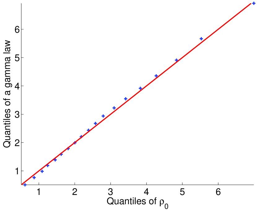
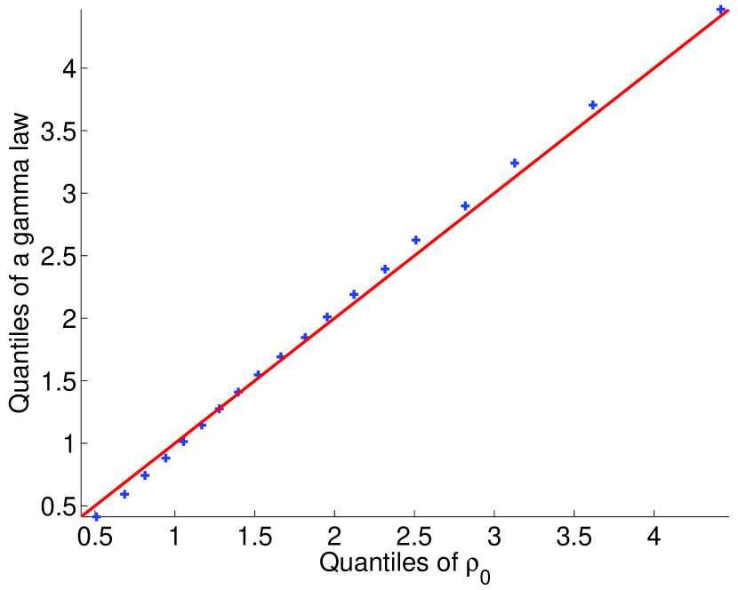
(a) η=2.5𝜂2.5\eta=2.5, λ=1BS/km2𝜆1superscriptBS/km2\lambda=1\text{BS/km}^{2}
Refer to caption
(b) η=3.2𝜂3.2\eta=3.2, λ=1BS/km2𝜆1superscriptBS/km2\lambda=1\text{BS/km}^{2}
Refer to caption
(c) η=4𝜂4\eta=4, λ=1BS/km2𝜆1superscriptBS/km2\lambda=1\text{BS/km}^{2}
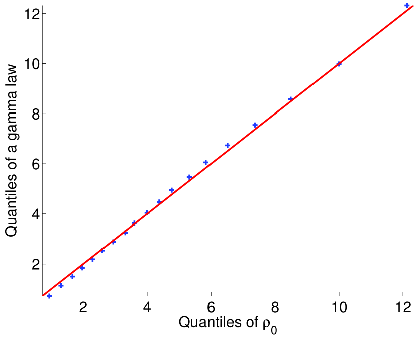
Figure 1: Quantile-to-Quantile comparison between the loads distribution and a gamma distribution

On figure 1 we compare the distribution of the loads obtained by simulation to a gamma distribution with the same mean and variance for η{2.5,3.2,4}𝜂2.53.24\eta\in\{2.5,3.2,4\} using a quantile-to-quantile plot. For the three values of η𝜂\eta we observe a good fit between the two. It is noted that from the results of [15], even the area of the Voronoi cell does not follow a gamma distribution, so in general the load cannot be gamma distributed. For practical purposes however, the gamma distribution provides a good approximation.

It is noted that choosing a gamma distribution with the same mean and variance is not the maximum likelihood estimation, since the maximum likelihood involves the expectation of the logarithm of the load. We use this moment estimator because we only know the mean and variance of the loads by Theorems 4 and 5. We recall that from corollary 6 the load distribution becomes heavy-tailed (𝔼0[ρ0]+superscript𝔼0delimited-[]subscript𝜌0\mathbb{E}^{0}\left[\rho_{0}\right]\to+\infty) when η2+𝜂superscript2\eta\to 2^{+}, so that it cannot be approximated by a light-tailed distribution such as the gamma in this case.

VI-B Average loads

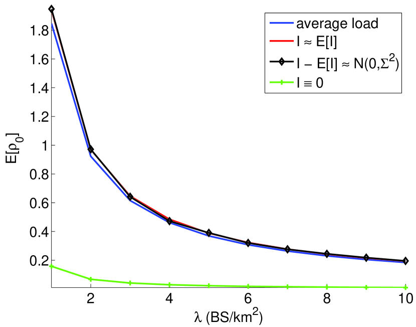
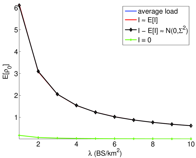
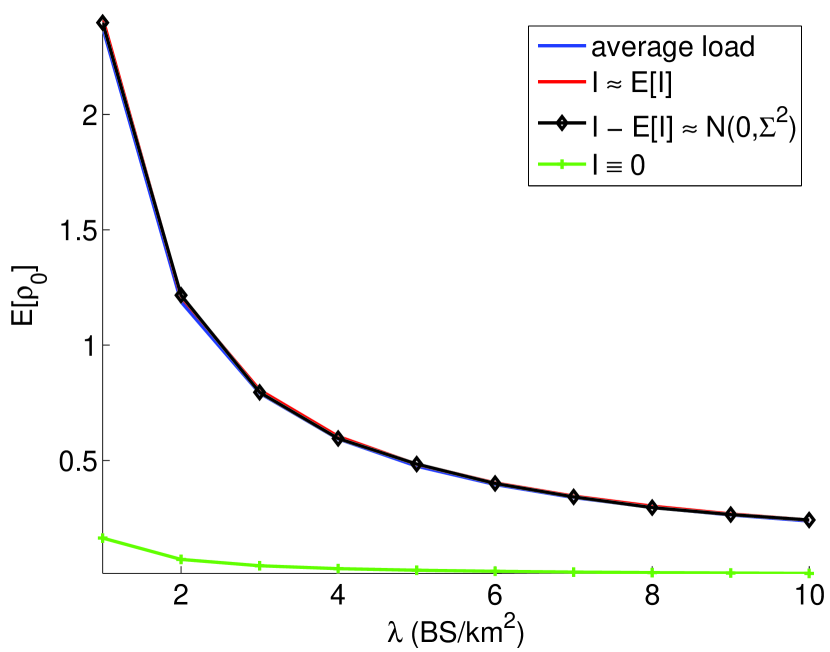
On figure 3, we plot the average load as a function of the BS density λ𝜆\lambda with η{2.5,3.5,4}𝜂2.53.54\eta\in\{2.5,3.5,4\}. The four curves are denoted:

  • a) “Average load”: the average load calculated by (8) of theorem 4,

  • b) “IE[I]𝐼𝐸delimited-[]𝐼I\approx E[I]”: an approximation of the average load by replacing the interference at a given location (z)𝑧{\cal I}(z) by its expectation 𝔼[(z)|z]𝔼delimited-[]conditional𝑧𝑧\mathbb{E}\left[{\cal I}(z)|z\right] .

  • c) “IE[I]N(0,Σ)𝐼𝐸delimited-[]𝐼𝑁0ΣI-E[I]\approx N(0,\Sigma)”: an approximation of the average load by replacing the interference at a given location (z)𝑧{\cal I}(z) by a normally distributed r.v. with variance given by corollary 7.

  • d) “I0𝐼0I\equiv 0”: the average load when there is no interference, i.e (z)0𝑧0{\cal I}(z)\equiv 0.

When λ𝜆\lambda increases, the interference increases, but the size of the typical cell decreases so that the amount of traffic served by a given BS decreases. Namely there is more interference but less congestion. On all curves, the average load decreases with λ𝜆\lambda which shows that the effect of reduced congestion dominates the effect of increased interference.

We observe that approximations b) and c) are fairly accurate, and that the accuracy is better when η𝜂\eta is close to 222. This is because, when η𝜂\eta decreases, the ratio between interference and path loss 𝔼[(z)|z]h(z)𝔼delimited-[]conditional𝑧𝑧𝑧\frac{\mathbb{E}\left[{\cal I}(z)|z\right]}{h(z)} increases, we get closer to the low SINR regime and If(z,I)𝐼𝑓𝑧𝐼I\to f(z,I) becomes closer to a linear function as explained in subsection III-B. The same argument also justifies the fact that for a given value of λ𝜆\lambda, the average load increases when the path-loss exponent η𝜂\eta decreases.

There is a large difference between the load with interference a) and without d), showing that taking into account interference for predicting the loads distribution is indeed necessary.
Refer to caption
(a) η=2.5𝜂2.5\eta=2.5
Refer to caption
(b) η=3.5𝜂3.5\eta=3.5
Refer to caption
(c) η=4𝜂4\eta=4
Figure 2: Average load as a function of the BS density λ𝜆\lambda

VI-C Frequency reuse

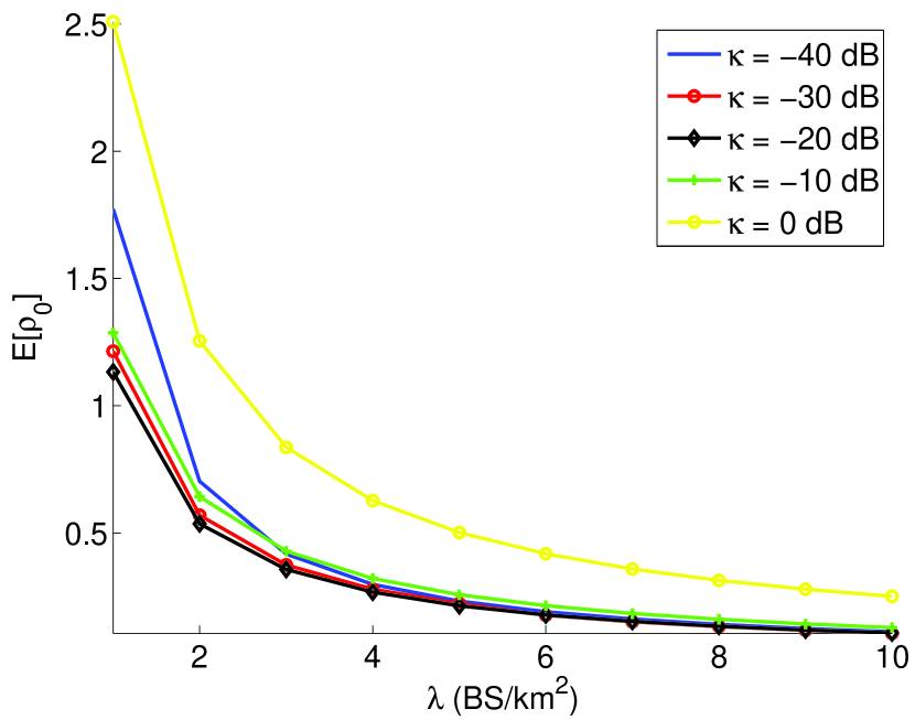
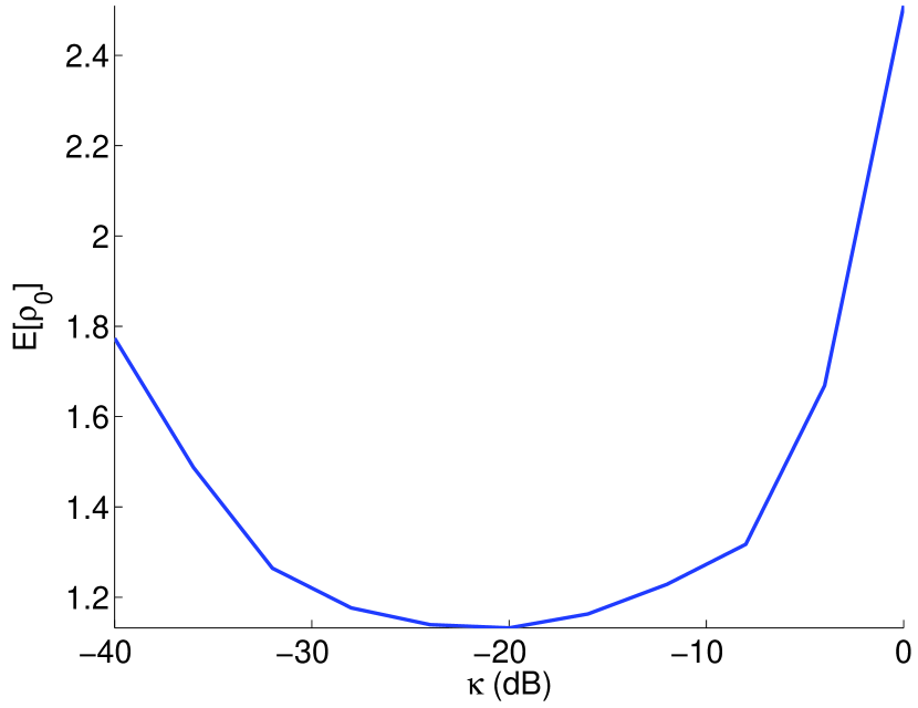
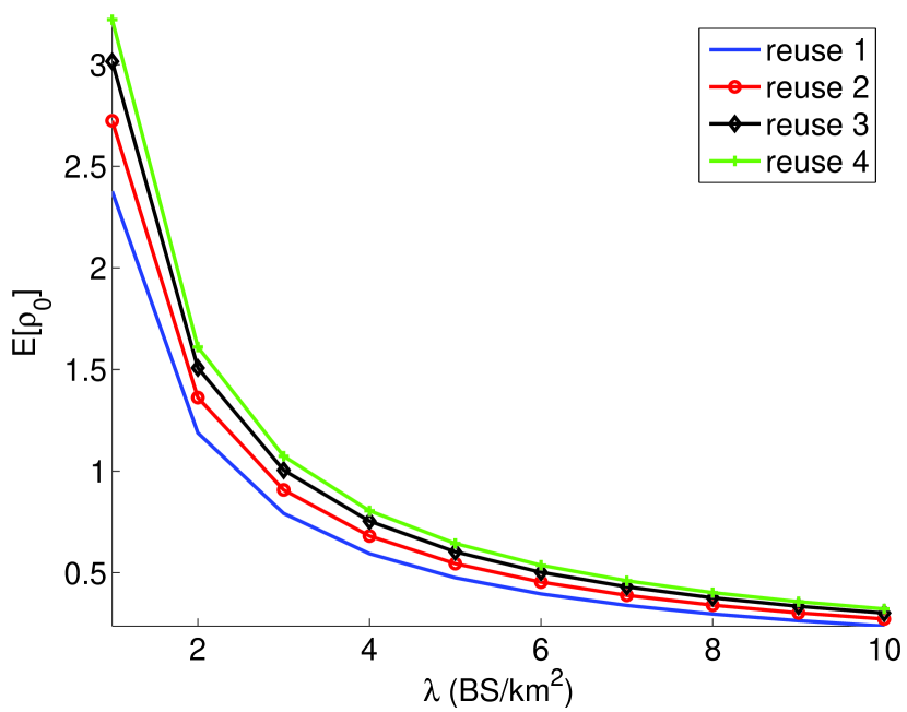
On figure 3, we plot the average load as a function of λ𝜆\lambda for different frequency reuse strategies as explained in subsection III-B4. On figure 3(a) we consider hard reuse with reuse factor b{1,,4}𝑏14b\in\{1,\dots,4\}. On figure 3(b) we consider soft reuse with b=3𝑏3b=3 and κ[40,0]𝜅400\kappa\in[-40,0] dB. For each value of λ𝜆\lambda and κ𝜅\kappa, the threshold between edge and center redgesubscript𝑟𝑒𝑑𝑔𝑒r_{edge} is chosen so that the average load of the center and edge are equal: 𝔼0[ρ0edge]=𝔼0[ρ0center]superscript𝔼0delimited-[]superscriptsubscript𝜌0𝑒𝑑𝑔𝑒superscript𝔼0delimited-[]superscriptsubscript𝜌0𝑐𝑒𝑛𝑡𝑒𝑟\mathbb{E}^{0}\left[\rho_{0}^{edge}\right]=\mathbb{E}^{0}\left[\rho_{0}^{center}\right]. On figure 3(c) we consider a soft reuse with b=3𝑏3b=3, λ=1BS/km2𝜆1superscriptBS/km2\lambda=1\text{BS/km}^{2} and κ[40,0]𝜅400\kappa\in[-40,0] dB.

We see that hard reuse schemes actually diminish the network performance by increasing the average load. Reuse 111 gives the best performance. This is true regardless of the BS density λ𝜆\lambda. On the other hand, soft reuse schemes bring considerable improvement. The value κ=20𝜅20\kappa=-20 dB gives the best performance, and the average load for this value is about half of the average load for reuse 111. This shows that for PPP networks, soft frequency reuse allows to serve twice as much traffic with the same number of BS.

Those results are in line with previous work such as [40] where the capacity of a regular network (possibly with small random perturbations) serving elastic traffic was studied. Namely soft reuse increases the network performance noticeably, while hard reuse brings little to no improvement. A noticeable difference though is that the optimal power reduction for the completely random PPP networks κ𝜅\kappa is 2020-20 dB, while for regular networks it is around 55-5 dB. Namely there is more than an order of magnitude of difference.
Refer to caption
(a) Hard reuse, η=3.5𝜂3.5\eta=3.5
Refer to caption
(b) Soft reuse 333, η=3.5𝜂3.5\eta=3.5
Refer to caption
(c) Soft reuse 333, η=3.5𝜂3.5\eta=3.5, λ=1BS/km2𝜆1superscriptBS/km2\lambda=1\text{BS/km}^{2}:
optimal κ𝜅\kappa
Figure 3: Average load for different frequency reuse strategies

VII Conclusion

We have considered the flow-level performance of random wireless networks. The locations of BS follow a PPP. We take into account flow-level dynamics by modeling each BS as a queue. The performance and stability of each BS depends on its load. In certain cases the full distribution of the load has been derived through its Laplace transform. In all cases, we have given formulas to calculate the first and second moments of the loads. Networks on the line and on the plane have both been considered. Our model is generic enough to include features of recent wireless networks such as 4G networks (LTE). In dense networks, we have shown that the inter-cell interference power becomes normally distributed. Hence some computations reduce to an integral with respect to the Gaussian distribution. Using numerical experiments we have demonstrated that in certain cases of practical interest, the loads distribution can be approximated by a gamma distribution with known mean and variance, and that this approximation is very accurate.

Acknowledgment

The authors are thankful to Alexandre Proutière for his helpful comments on the traffic models.

References

  • [1] F. Baccelli and B. Blaszczyszyn, “Stochastic geometry and wireless networks, volume 1: Theory,” Foundations and Trends in Networking, vol. 3, no. 3-4, pp. 249–449, 2009.
  • [2] ——, “Stochastic geometry and wireless networks, volume 2: Applications,” Foundations and Trends in Networking, vol. 4, no. 1-2, pp. 1–312, 2009.
  • [3] J. Kaufman, “Blocking in a shared resource environment,” IEEE Transactions on Communications, vol. 29, no. 10, pp. 1474 – 1481, oct 1981.
  • [4] J. W. Roberts, “A service system with heterogeneous user requirements,” in Performance of Data Communications Systems and Their Applications, 1981, pp. 423–431.
  • [5] F. Baccelli, B. Blaszczyszyn, and M. K. Karray, “Blocking rates in large CDMA networks via a spatial erlang formula,” INRIA, Rapport de recherche RR-5517, 2005.
  • [6] T. Bonald and A. Proutière, “Wireless downlink data channels: User performance and cell dimensioning,” in Proceedings of ACM MOBICOM, 2003.
  • [7] E. Altman, “Capacity of multi-service cellular networks with transmission-rate control: a queueing analysis,” in Proceedings of ACM MOBICOM, 2002, pp. 205–214.
  • [8] T. Bonald and A. Proutière, “On performance bounds for the integration of elastic and adaptive streaming flows,” SIGMETRICS Perform. Eval. Rev., vol. 32, no. 1, pp. 235–245, Jun. 2004.
  • [9] E. N. Gilbert, “Random subdivisions of space into crystals,” The Annals of Mathematical Statistics, vol. 33, no. 3, pp. 958–972, 1962.
  • [10] T. Kiang, “Random Fragmentation in Two and Three Dimensions,” Zeitschrift für Astrophysik, vol. 64, p. 433, 1966.
  • [11] J.-S. Ferenc and Z. Néda, “On the size distribution of Poisson Voronoi cells,” Physica A Statistical Mechanics and its Applications, vol. 385, pp. 518–526, Nov. 2007.
  • [12] P. Calka, “The distributions of the smallest disks containing the Poisson-Voronoi typical cell and the Crofton cell in the plane,” Advances in Applied Probability, vol. 34, no. 4, pp. 702–717, 2002.
  • [13] ——, “An explicit expression for the distribution of the number of sides of the typical Poisson-Voronoi cell,” Advances in Applied Probability, vol. 35, no. 4, pp. 863–870, 2003.
  • [14] S. A. Zuyev, “Estimates for distributions of the Voronoi polygon’s geometric characteristics,” Random Struct. Algorithms, pp. 149–162, 1992.
  • [15] P. Calka, “Precise formulae for the distributions of the principal geometric characteristics of the typical cells of a two-dimensional Poisson-Voronoi tessellation and a Poisson line process,” Advances in Applied Probability, vol. 35, no. 3, pp. 551–562, 2003.
  • [16] J. Møller and S. Zuyev, “Gamma-type results and other related properties of Poisson processes,” Advances in Applied Probability, vol. 28, no. 3, pp. 662–673, 1996.
  • [17] S. G. Foss and S. A. Zuyev, “On a Voronoi aggregative process related to a bivariate Poisson process,” Advances in Applied Probability, vol. 28, no. 4, pp. 965–981, 1996.
  • [18] F. Baccelli, B. Blaszczyszyn, and F. Tournois, “Spatial averages of coverage characteristics in large CDMA networks,” Wireless Networks, vol. 8, no. 6, pp. 569–586, 2002.
  • [19] J. G. Andrews, F. Baccelli, and R. K. Ganti, “A tractable approach to coverage and rate in cellular networks,” IEEE Transactions on Communications, vol. 59, no. 11, pp. 3122–3134, Nov. 2011.
  • [20] T. Novlan, H. Dhillon, and J. Andrews, “Analytical modeling of uplink cellular networks,” IEEE Transactions on Wireless Communications, no. 99, pp. 1–11, 2013.
  • [21] S. Singh, H. Dhillon, and J. Andrews, “Offloading in heterogeneous networks: Modeling, analysis, and design insights,” IEEE Transactions on Wireless Communications, vol. 12, no. 5, pp. 2484–2497, 2013.
  • [22] H. Dhillon, R. Ganti, and J. Andrews, “Load-aware modeling and analysis of heterogeneous cellular networks,” IEEE Transactions on Wireless Communications, vol. 12, no. 4, pp. 1666–1677, 2013.
  • [23] H. Dhillon, R. Ganti, F. Baccelli, and J. Andrews, “Modeling and analysis of k-tier downlink heterogeneous cellular networks,” IEEE Journal on Selected Areas in Communications, vol. 30, no. 3, pp. 550–560, 2012.
  • [24] T. Novlan, R. Ganti, A. Ghosh, and J. Andrews, “Analytical evaluation of fractional frequency reuse for heterogeneous cellular networks,” IEEE Transactions on Communications, vol. 60, no. 7, pp. 2029–2039, 2012.
  • [25] X. Lin, J. G. Andrews, and A. Ghosh, “Modeling, analysis and design for carrier aggregation in heterogeneous cellular networks,” CoRR, vol. abs/1211.4041, 2012.
  • [26] H.-S. Jo, Y. J. Sang, P. Xia, and J. G. Andrews, “Heterogeneous cellular networks with flexible cell association: A comprehensive downlink SINR analysis,” CoRR, vol. abs/1107.3602, 2011.
  • [27] L. Decreusefond, P. Martins, and T.-T. Vu, “An analytical model for evaluating outage and handover probability of cellular wireless networks,” in Proceedings of WPMC, Taïwan, 2012, pp. 1–5.
  • [28] R. Ganti, F. Baccelli, and J. Andrews, “Series expansion for interference in wireless networks,” IEEE Transactions on Information Theory, vol. 58, no. 4, pp. 2194–2205, 2012.
  • [29] A. Guo and M. Haenggi, “Spatial Stochastic Models and Metrics for the Structure of Base Stations in Cellular Networks,” IEEE Transactions on Wireless Communications, 2013, submitted. Available at http://www.nd.edu/ mhaenggi/pubs/twc13b.pdf.
  • [30] S. M. Yu and S.-L. Kim, “Downlink capacity and base station density in cellular networks,” CoRR, vol. abs/1109.2992, 2011.
  • [31] S. Lowen and M. Teich, “Power-law shot noise,” IEEE Transactions on Information Theory, vol. 36, no. 6, pp. 1302 –1318, nov 1990.
  • [32] K. Gulati, B. Evans, J. Andrews, and K. Tinsley, “Statistics of co-channel interference in a field of Poisson and Poisson-Poisson clustered interferers,” IEEE Transactions on Signal Processing, vol. 58, no. 12, pp. 6207–6222, 2010.
  • [33] D. J. Dalay and D. Vere-Jones, An introduction to the theory of point processes.   Springer, 2002.
  • [34] L. Kleinrock, Queueing Systems: Theory.   Wiley, 1976, vol. 1.
  • [35] T. Bonald and M. Feuillet, Network Performance Analysis.   ISTE Ltd and John Wiley and Sons Inc, September 2011.
  • [36] P. Mogensen, W. Na, I. Kovacs, F. Frederiksen, A. Pokhariyal, K. Pedersen, T. Kolding, K. Hugl, and M. Kuusela, “LTE capacity compared to the Shannon bound,” in Proceedings of IEEE VTC, 2007, pp. 1234–1238.
  • [37] B. Błaszczyszyn and M. K. Karray, “Fading effect on the dynamic performance evaluation of OFDMA cellular networks,” in Proceedings of ComNet, 2009.
  • [38] R. Combes, Z. Altman, and E. Altman, “Scheduling gain for frequency-selective rayleigh-fading channels with application to self-organizing packet scheduling,” Performance Evaluation, Feb. 2011.
  • [39] S. Borst, “User-level performance of channel-aware scheduling algorithms in wireless data networks,” IEEE/ACM Transactions on Networking, vol. 13, no. 3, pp. 636–647, Jun. 2005.
  • [40] T. Bonald and N. Hegde, “Capacity gains of some frequency reuse schemes in OFDMA networks,” in Proceedings of IEEE GLOBECOM, dec. 2009, pp. 1–6.
  • [41] T. Bonald, S. Borst, N. Hegde, and A. Proutière, “Wireless data performance in multi-cell scenarios,” in Proceedings of ACM SIGMETRICS, 2004, pp. 378–387.
  • [42] D. Tsilimantos, J.-M. Gorce, and E. Altman, “Stochastic Analysis of Energy Savings with Sleep Mode in OFDMA Wireless Networks,” in Proceedings of IEEE INFOCOM, 2013.
  • [43] W. Weibull, “A statistical distribution function of wide applicability,” Journal of Applied Mechanics, vol. 18, pp. 293–297, 1951.
  • [44] F. Yilmaz and M.-S. Alouini, “Sum of Weibull variates and performance of diversity systems,” in Proceedings of IWCMC, 2009, pp. 247–252.
  • [45] W. Davenport and W. Root, An introduction to the theory of random signals and noise, ser. Lincoln Laboratory publications.   McGraw-Hill, 1958.
  • [46] W. Feller, An introduction to probability theory and its applications, ser. Wiley series in probability and mathematical statistics. Probability and mathematical statistics.   Wiley, 1966.
  • [47] C. Gloaguen, F. Fleischer, H. Schmidt, and V. Schmidt, “Simulation of typical Cox-Voronoi cells with a special regard to implementation tests,” Math. Meth. of OR, vol. 62, no. 3, pp. 357–373, 2005.

Appendix A Auxiliary results on shot noise generated by a PPP

A-A Laplace transform of shot noise

The Laplace transform of shot noise is given by Theorem 2. A proof can be found for instance in [1].

Proposition 2.

Consider ΦΦ\Phi a PPP on M𝑀M with measure λ(dz)𝜆𝑑𝑧\lambda(dz). for all N1𝑁1N\geq 1, (z1,,zN)MNsubscript𝑧1subscript𝑧𝑁superscript𝑀𝑁(z_{1},\cdots,z_{N})\in M^{N}, (s1,,sN)Nsubscript𝑠1subscript𝑠𝑁superscript𝑁(s_{1},\cdots,s_{N})\in\mathbb{C}^{N}: with strictly positive real part:

𝔼[exp(i=1Nsi(zi))]𝔼delimited-[]superscriptsubscript𝑖1𝑁subscript𝑠𝑖subscript𝑧𝑖\displaystyle\mathbb{E}\left[\exp(-\sum_{i=1}^{N}s_{i}{\cal I}(z_{i}))\right]
=exp{M[1𝒢(sii=1Nh(ziz))]λ(dz)}.absentsubscript𝑀delimited-[]1𝒢subscript𝑠𝑖superscriptsubscript𝑖1𝑁delimited-∥∥subscript𝑧𝑖𝑧𝜆𝑑𝑧\displaystyle=\exp\left\{-\int_{M}\left[1-{\cal G}\left(s_{i}\sum_{i=1}^{N}h(\lVert z_{i}-z\rVert)\right)\right]\lambda(dz)\right\}.

A-B Expectation of a function of shot noise

It is noted that once the Fourier/Laplace transform of a random variable I𝐼I is known, the expectation of any function of I𝐼I can be calculated using the Plancherel-Parseval theorem recalled in proposition 3.

Proposition 3 (Plancherel theorem).

Consider I𝐼I a real random variable and f𝑓f a positive function:

𝔼[f(I)]=f^(s)¯𝔼[exp(siI)]𝑑s.𝔼delimited-[]𝑓𝐼subscript¯^𝑓𝑠𝔼delimited-[]𝑠𝑖𝐼differential-d𝑠\mathbb{E}\left[f(I)\right]=\int_{\mathbb{R}}\overline{\hat{f}(s)}\mathbb{E}\left[\exp(-siI)\right]ds.

with f^^𝑓\hat{f} the Fourier transform of f𝑓f, and z¯¯𝑧\overline{z} the complex conjugate of z𝑧z.

It is noted that if f𝑓f is not square integrable, the Fourier transform should be taken in the sense of tempered distributions.

A-C Shot noise distributions of interest

We can specialize Theorem 2 to obtain results on the distribution of shot noise generated by an homogenous PPP, conditional to the event z𝒞(0)𝑧𝒞0z\in{\cal C}(0).

Proposition 4.

The Laplace transform of (z)𝑧{\cal I}(z), conditional to z𝒞(0)𝑧𝒞0z\in{\cal C}(0) is:

𝔼[exp(s(z))|z]=exp(2πλ|z|+r(1𝒢(sh(r)))𝑑r).𝔼delimited-[]conditional𝑠𝑧𝑧2𝜋𝜆superscriptsubscript𝑧𝑟1𝒢𝑠𝑟differential-d𝑟\mathbb{E}\left[\exp(-s{\cal I}(z))|z\right]=\exp\left(-2\pi\lambda\int_{\lvert z\rvert}^{+\infty}r(1-{\cal G}(sh(r)))dr\right).

and its first and second moments are:

𝔼[(z)|z]𝔼delimited-[]conditional𝑧𝑧\displaystyle\mathbb{E}\left[{\cal I}(z)|z\right] =2πλ𝔼[G]|z|+rh(r)𝑑r,absent2𝜋𝜆𝔼delimited-[]𝐺superscriptsubscript𝑧𝑟𝑟differential-d𝑟\displaystyle=2\pi\lambda\mathbb{E}\left[G\right]\int_{\lvert z\rvert}^{+\infty}rh(r)dr,
𝐯𝐚𝐫((z)|z)𝐯𝐚𝐫conditional𝑧𝑧\displaystyle{\bf var}({\cal I}(z)|z) =2πλ𝔼[G2]|z|+rh(r)2𝑑r,absent2𝜋𝜆𝔼delimited-[]superscript𝐺2superscriptsubscript𝑧𝑟superscript𝑟2differential-d𝑟\displaystyle=2\pi\lambda\mathbb{E}\left[G^{2}\right]\int_{\lvert z\rvert}^{+\infty}rh(r)^{2}dr,
Proof.

By specialization of theorem 2 to N=1𝑁1N=1 and λ(dx)=λ𝟏1(z)(x)dx𝜆𝑑𝑥𝜆subscript1subscript1𝑧𝑥𝑑𝑥\lambda(dx)=\lambda{\bf 1}_{\mathbb{C}\setminus{\cal B}_{1}(z)}(x)dx:

𝔼[exp(s(z))|z])\displaystyle\mathbb{E}\left[\exp(-s{\cal I}(z))|z\right])
=exp(λ1(z)(1𝒢(sh(zx)))𝑑x).absent𝜆subscriptsubscript1𝑧1𝒢𝑠𝑧𝑥differential-d𝑥\displaystyle=\exp\left(-\lambda\int_{\mathbb{C}\setminus{\cal B}_{1}(z)}(1-{\cal G}(sh(z-x)))dx\right).

Once again, using polar coordinates and centering (i.e zx=reiθ𝑧𝑥𝑟superscript𝑒𝑖𝜃z-x=re^{i\theta}) gives the result:

𝔼[exp(s(z))|z]=exp(2πλ|z|+(1𝒢(sh(r)))r𝑑r).𝔼delimited-[]conditional𝑠𝑧𝑧2𝜋𝜆superscriptsubscript𝑧1𝒢𝑠𝑟𝑟differential-d𝑟\mathbb{E}\left[\exp(-s{\cal I}(z))|z\right]=\exp\left(-2\pi\lambda\int_{\lvert z\rvert}^{+\infty}(1-{\cal G}(sh(r)))rdr\right).

Proposition 5.

With assumptions 1, the Laplace transform of (z)𝑧{\cal I}(z), conditional to z𝒞(0)𝑧𝒞0z\in{\cal C}(0) is given by:

log(𝔼[exp(s(z))|z])𝔼delimited-[]conditional𝑠𝑧𝑧\displaystyle\log(\mathbb{E}\left[\exp(s{\cal I}(z))|z\right])
=πλ[|z|2+2(Ps)2ηγ(Ps|z|η,2/η)/η],absent𝜋𝜆delimited-[]superscript𝑧22superscript𝑃𝑠2𝜂𝛾𝑃𝑠superscript𝑧𝜂2𝜂𝜂\displaystyle=\pi\lambda\left[\lvert z\rvert^{2}\right.+\left.2(Ps)^{\frac{2}{\eta}}\gamma(Ps\lvert z\rvert^{-\eta},-2/\eta)/\eta\right],

with γ(x,s)=0xts1et𝑑t𝛾𝑥𝑠superscriptsubscript0𝑥superscript𝑡𝑠1superscript𝑒𝑡differential-d𝑡\gamma(x,s)=\int_{0}^{x}t^{s-1}e^{-t}dt the lower incomplete gamma function and Γ(s)=Γ(+,s)Γ𝑠Γ𝑠\Gamma(s)=\Gamma(+\infty,s) the gamma function. Its first and second moments are:

𝔼[(z)|z]𝔼delimited-[]conditional𝑧𝑧\displaystyle\mathbb{E}\left[{\cal I}(z)|z\right] =2πλ𝔼[G]Pr2η/(η2),absent2𝜋𝜆𝔼delimited-[]𝐺𝑃superscript𝑟2𝜂𝜂2\displaystyle=2\pi\lambda\mathbb{E}\left[G\right]Pr^{2-\eta}/(\eta-2),
𝐯𝐚𝐫((z)|z)𝐯𝐚𝐫conditional𝑧𝑧\displaystyle{\bf var}({\cal I}(z)|z) =2πλ𝔼[G2]P2r22η/(2η2).absent2𝜋𝜆𝔼delimited-[]superscript𝐺2superscript𝑃2superscript𝑟22𝜂2𝜂2\displaystyle=2\pi\lambda\mathbb{E}\left[G^{2}\right]P^{2}r^{2-2\eta}/(2\eta-2).
Proof.

See [19]. ∎

Appendix B Proofs

B-A Proof of theorem 1

Proof.

First assume (xl,xr)subscript𝑥𝑙subscript𝑥𝑟(x_{l},x_{r}) to be known. We decompose the load (4) in two terms using (5) and the symmetry of f0subscript𝑓0f_{0}:

ρ0subscript𝜌0\displaystyle\rho_{0} =xl/2xr/2f0(z)𝑑z=0xr/2f0(z)𝑑z+0xl/2f0(z)𝑑zabsentsuperscriptsubscriptsubscript𝑥𝑙2subscript𝑥𝑟2subscript𝑓0𝑧differential-d𝑧superscriptsubscript0subscript𝑥𝑟2subscript𝑓0𝑧differential-d𝑧superscriptsubscript0subscript𝑥𝑙2subscript𝑓0𝑧differential-d𝑧\displaystyle=\int_{-x_{l}/2}^{x_{r}/2}f_{0}(z)dz=\int_{0}^{x_{r}/2}f_{0}(z)dz+\int_{0}^{x_{l}/2}f_{0}(z)dz
=F0(xl/2)+F0(xr/2).absentsubscript𝐹0subscript𝑥𝑙2subscript𝐹0subscript𝑥𝑟2\displaystyle=F_{0}(x_{l}/2)+F_{0}(x_{r}/2).

By proposition 1, (xl,xr)subscript𝑥𝑙subscript𝑥𝑟(x_{l},x_{r}) are i.i.d. so that:

𝔼0[exp(sρ0)]superscript𝔼0delimited-[]𝑠subscript𝜌0\displaystyle\mathbb{E}^{0}\left[\exp(-s\rho_{0})\right] =𝔼0[exp(s(F0(xl/2)+F0(xr/2)))]absentsuperscript𝔼0delimited-[]𝑠subscript𝐹0subscript𝑥𝑙2subscript𝐹0subscript𝑥𝑟2\displaystyle=\mathbb{E}^{0}\left[\exp(-s(F_{0}(x_{l}/2)+F_{0}(x_{r}/2)))\right]
=(𝔼0[exp(sF0(xl/2))])2.absentsuperscriptsuperscript𝔼0delimited-[]𝑠subscript𝐹0subscript𝑥𝑙22\displaystyle=(\mathbb{E}^{0}\left[\exp(-sF_{0}(x_{l}/2))\right])^{2}. (11)

xlsubscript𝑥𝑙x_{l} is exponentially distributed with parameter λ𝜆\lambda so that the r.h.s. of (B-A) equals:

𝔼0[exp(sρ0)]superscript𝔼0delimited-[]𝑠subscript𝜌0\displaystyle\mathbb{E}^{0}\left[\exp(-s\rho_{0})\right]
=(λ0+exp(sF0(r/2))exp(rλ)𝑑r)2,absentsuperscript𝜆superscriptsubscript0𝑠subscript𝐹0𝑟2𝑟𝜆differential-d𝑟2\displaystyle=\left(\lambda\int_{0}^{+\infty}\exp(-sF_{0}(r/2))\exp(-r\lambda)dr\right)^{2},

proving the result. ∎

B-B Proof of theorem 2

Proof.

We first consider (xl,xr)subscript𝑥𝑙subscript𝑥𝑟(x_{l},x_{r}) to be known. The interference at z𝒞(0)𝑧𝒞0z\in{\cal C}(0) can be decomposed into:

(z)𝑧\displaystyle{\cal I}(z) =G1h(|z+xl|)+G1h(|zxr|)absentsubscript𝐺1𝑧subscript𝑥𝑙subscript𝐺1𝑧subscript𝑥𝑟\displaystyle=G_{-1}h(\lvert z+x_{l}\rvert)+G_{1}h(\lvert z-x_{r}\rvert)
+n{1,0,1}Gnh(|zxn|).subscript𝑛101subscript𝐺𝑛𝑧subscript𝑥𝑛\displaystyle+\sum_{n\in\mathbb{N}\setminus\{-1,0,1\}}G_{n}h(\lvert z-x_{n}\rvert).

The interference dependent term in (6) can be written:

xl/2xr/2f1(z)superscriptsubscriptsubscript𝑥𝑙2subscript𝑥𝑟2subscript𝑓1𝑧\displaystyle\int_{-x_{l}/2}^{x_{r}/2}f_{1}(z) (z)dz=G1xl/2xr/2f1(z)h(|z+xl|)𝑑z𝑧𝑑𝑧subscript𝐺1superscriptsubscriptsubscript𝑥𝑙2subscript𝑥𝑟2subscript𝑓1𝑧𝑧subscript𝑥𝑙differential-d𝑧\displaystyle{\cal I}(z)dz=G_{-1}\int_{-x_{l}/2}^{x_{r}/2}f_{1}(z)h(\lvert z+x_{l}\rvert)dz
+G1xl/2xr/2f1(z)h(|zxr|)𝑑zsubscript𝐺1superscriptsubscriptsubscript𝑥𝑙2subscript𝑥𝑟2subscript𝑓1𝑧𝑧subscript𝑥𝑟differential-d𝑧\displaystyle+G_{1}\int_{-x_{l}/2}^{x_{r}/2}f_{1}(z)h(\lvert z-x_{r}\rvert)dz
+n{1,0,1}Gnxl/2xr/2f1(z)h(|zxn|)𝑑z.subscript𝑛101subscript𝐺𝑛superscriptsubscriptsubscript𝑥𝑙2subscript𝑥𝑟2subscript𝑓1𝑧𝑧subscript𝑥𝑛differential-d𝑧\displaystyle+\sum_{n\in\mathbb{N}\setminus\{-1,0,1\}}G_{n}\int_{-x_{l}/2}^{x_{r}/2}f_{1}(z)h(\lvert z-x_{n}\rvert)dz. (12)

By definition of 𝒦𝒦{\cal K} (eq. IV-C), the r.h.s. of (B-B) becomes:

xl/2xr/2f1(z)(z)𝑑zsuperscriptsubscriptsubscript𝑥𝑙2subscript𝑥𝑟2subscript𝑓1𝑧𝑧differential-d𝑧\displaystyle\int_{-x_{l}/2}^{x_{r}/2}f_{1}(z){\cal I}(z)dz =G1𝒦(xl,xl,xr)+G1𝒦(xr,xl,xr)absentsubscript𝐺1𝒦subscript𝑥𝑙subscript𝑥𝑙subscript𝑥𝑟subscript𝐺1𝒦subscript𝑥𝑟subscript𝑥𝑙subscript𝑥𝑟\displaystyle=G_{-1}{\cal K}(-x_{l},x_{l},x_{r})+G_{1}{\cal K}(x_{r},x_{l},x_{r})
+n{1,0,1}Gn𝒦(xn,rl,rr).subscript𝑛101subscript𝐺𝑛𝒦subscript𝑥𝑛subscript𝑟𝑙subscript𝑟𝑟\displaystyle+\sum_{n\in\mathbb{N}\setminus\{-1,0,1\}}G_{n}{\cal K}(x_{n},r_{l},r_{r}). (13)

The third term on the r.h.s. of (B-B) is a shot noise with respect to the point process Φ[xl,xr]Φsubscript𝑥𝑙subscript𝑥𝑟\Phi\setminus[-x_{l},x_{r}], with impulse response z𝒦(z,xl,xr)maps-to𝑧𝒦𝑧subscript𝑥𝑙subscript𝑥𝑟z\mapsto{\cal K}(z,x_{l},x_{r}). Conditional to (xl,xr)subscript𝑥𝑙subscript𝑥𝑟(x_{l},x_{r}), Φ[xl,xr]Φsubscript𝑥𝑙subscript𝑥𝑟\Phi\setminus[-x_{l},x_{r}] is a PPP on [xl,xr]subscript𝑥𝑙subscript𝑥𝑟\mathbb{R}\setminus[-x_{l},x_{r}] with intensity λ𝜆\lambda. Hence we can apply proposition 2:

𝔼0[exp{sn{1,0,1}Gn𝒦(xn,rl,rr)}|xl,xr]superscript𝔼0delimited-[]conditional𝑠subscript𝑛101subscript𝐺𝑛𝒦subscript𝑥𝑛subscript𝑟𝑙subscript𝑟𝑟subscript𝑥𝑙subscript𝑥𝑟\displaystyle\mathbb{E}^{0}\left[\exp\left\{-s\sum_{n\in\mathbb{N}\setminus\{-1,0,1\}}G_{n}{\cal K}(x_{n},r_{l},r_{r})\right\}|x_{l},x_{r}\right]
=exp{λ[rl,rr](1𝒢(s𝒦(z,rl,rr)))𝑑z}absent𝜆subscriptsubscript𝑟𝑙subscript𝑟𝑟1𝒢𝑠𝒦𝑧subscript𝑟𝑙subscript𝑟𝑟differential-d𝑧\displaystyle=\exp\left\{-\lambda\int_{\mathbb{R}\setminus[-r_{l},r_{r}]}(1-{\cal G}(s{\cal K}(z,r_{l},r_{r})))dz\right\} (14)

Furthermore, the Laplace transform of the two first terms of (B-B) is:

𝔼0[exp(sG1𝒦(xl,xl,xr)sG1𝒦(xr,xl,xr))|xl,xr]superscript𝔼0delimited-[]conditional𝑠subscript𝐺1𝒦subscript𝑥𝑙subscript𝑥𝑙subscript𝑥𝑟𝑠subscript𝐺1𝒦subscript𝑥𝑟subscript𝑥𝑙subscript𝑥𝑟subscript𝑥𝑙subscript𝑥𝑟\displaystyle\mathbb{E}^{0}\left[\exp(-sG_{-1}{\cal K}(-x_{l},x_{l},x_{r})-sG_{1}{\cal K}(x_{r},x_{l},x_{r}))|x_{l},x_{r}\right]
=𝒢(s𝒦(xl,xl,xr))𝒢(s𝒦(xr,xl,xr)).absent𝒢𝑠𝒦subscript𝑥𝑙subscript𝑥𝑙subscript𝑥𝑟𝒢𝑠𝒦subscript𝑥𝑟subscript𝑥𝑙subscript𝑥𝑟\displaystyle={\cal G}(s{\cal K}(-x_{l},x_{l},x_{r})){\cal G}(s{\cal K}(x_{r},x_{l},x_{r})). (15)

Combining (B-B) and (B-B) we obtain the Laplace transform of the interference dependent term in (6):

𝔼0[exp(sxl/2xr/2f1(z)(z)𝑑z)|xl,xr]superscript𝔼0delimited-[]conditional𝑠superscriptsubscriptsubscript𝑥𝑙2subscript𝑥𝑟2subscript𝑓1𝑧𝑧differential-d𝑧subscript𝑥𝑙subscript𝑥𝑟\displaystyle\mathbb{E}^{0}\left[\exp\left(-s\int_{-x_{l}/2}^{x_{r}/2}f_{1}(z){\cal I}(z)dz\right)|x_{l},x_{r}\right]
=𝒢(s𝒦(xl,xl,xr))𝒢(s𝒦(xr,xl,xr))absent𝒢𝑠𝒦subscript𝑥𝑙subscript𝑥𝑙subscript𝑥𝑟𝒢𝑠𝒦subscript𝑥𝑟subscript𝑥𝑙subscript𝑥𝑟\displaystyle={\cal G}(s{\cal K}(-x_{l},x_{l},x_{r})){\cal G}(s{\cal K}(x_{r},x_{l},x_{r}))
exp[λ[xl,xr](1𝒢(s𝒦(z,xl,xr)))𝑑z]𝜆subscriptsubscript𝑥𝑙subscript𝑥𝑟1𝒢𝑠𝒦𝑧subscript𝑥𝑙subscript𝑥𝑟differential-d𝑧\displaystyle\exp\left[-\lambda\int_{\mathbb{R}\setminus[-x_{l},x_{r}]}(1-{\cal G}(s{\cal K}(z,x_{l},x_{r})))dz\right]
=(s,xl,xr).absent𝑠subscript𝑥𝑙subscript𝑥𝑟\displaystyle={\cal L}(s,x_{l},x_{r}).

The Laplace transform of the load conditional to (xl,xr)subscript𝑥𝑙subscript𝑥𝑟(x_{l},x_{r}) is then:

𝔼0[exp(sρ0)|xl,xr]superscript𝔼0delimited-[]conditional𝑠subscript𝜌0subscript𝑥𝑙subscript𝑥𝑟\displaystyle\mathbb{E}^{0}\left[\exp(-s\rho_{0})|x_{l},x_{r}\right]
=(s,xl,xr)exp(s(F0(xl/2)+F0(xr/2))).absent𝑠subscript𝑥𝑙subscript𝑥𝑟𝑠subscript𝐹0subscript𝑥𝑙2subscript𝐹0subscript𝑥𝑟2\displaystyle={\cal L}(s,x_{l},x_{r})\exp(-s(F_{0}(x_{l}/2)+F_{0}(x_{r}/2))). (16)

Since (xl,xr)subscript𝑥𝑙subscript𝑥𝑟(x_{l},x_{r}) are i.i.d. and exponentially distributed, the load distribution is obtained by un-conditioning (B-B):

𝔼0[exp(sρ0)]=λ22(s,r1,r2)superscript𝔼0delimited-[]𝑠subscript𝜌0superscript𝜆2subscriptsuperscript2𝑠subscript𝑟1subscript𝑟2\displaystyle\mathbb{E}^{0}\left[\exp(-s\rho_{0})\right]=\lambda^{2}\int_{\mathbb{R}^{2}}{\cal L}(s,r_{1},r_{2})
exp{λ(r1+r2)s(F0(r1/2)+F0(r2/2))}dr1dr2.𝜆subscript𝑟1subscript𝑟2𝑠subscript𝐹0subscript𝑟12subscript𝐹0subscript𝑟22𝑑subscript𝑟1𝑑subscript𝑟2\displaystyle\exp\left\{-\lambda(r_{1}+r_{2})-s(F_{0}(r_{1}/2)+F_{0}(r_{2}/2))\right\}dr_{1}dr_{2}. (17)

The expression under the integral in (B-B) is symmetrical in (r1,r2)subscript𝑟1subscript𝑟2(r_{1},r_{2}) which proves the result. ∎

B-C Proof of Theorem 3

Proof.

We first write the definition of the load:

ρ0Nsuperscriptsubscript𝜌0𝑁\displaystyle\rho_{0}^{N} =(f(z,(z))𝟏𝒞(0)(z)𝑑z)Nabsentsuperscriptsubscript𝑓𝑧𝑧subscript1𝒞0𝑧differential-d𝑧𝑁\displaystyle=\left(\int_{\mathbb{C}}f(z,{\cal I}(z)){\bf 1}_{{\cal C}(0)}(z)dz\right)^{N}
=N[i=1Nf(zi,(zi))]𝟏𝒞(0)N(z1,,zN)𝑑z1𝑑zN.absentsubscriptsuperscript𝑁delimited-[]superscriptsubscriptproduct𝑖1𝑁𝑓subscript𝑧𝑖subscript𝑧𝑖subscript1𝒞superscript0𝑁subscript𝑧1subscript𝑧𝑁differential-dsubscript𝑧1differential-dsubscript𝑧𝑁\displaystyle=\int_{\mathbb{C}^{N}}\left[\prod_{i=1}^{N}f(z_{i},{\cal I}(z_{i}))\right]{\bf 1}_{{\cal C}(0)^{N}}(z_{1},\cdots,z_{N})dz_{1}\cdots dz_{N}.

Taking expectations:

𝔼0[ρ0N]superscript𝔼0delimited-[]superscriptsubscript𝜌0𝑁\displaystyle\mathbb{E}^{0}\left[\rho_{0}^{N}\right]
=N𝔼0[[i=1Nf(zi,(zi))]𝟏𝒞(0)N(z1,,zN)]𝑑z1𝑑zN.absentsubscriptsuperscript𝑁superscript𝔼0delimited-[]delimited-[]superscriptsubscriptproduct𝑖1𝑁𝑓subscript𝑧𝑖subscript𝑧𝑖subscript1𝒞superscript0𝑁subscript𝑧1subscript𝑧𝑁differential-dsubscript𝑧1differential-dsubscript𝑧𝑁\displaystyle=\int_{\mathbb{C}^{N}}\mathbb{E}^{0}\left[\left[\prod_{i=1}^{N}f(z_{i},{\cal I}(z_{i}))\right]{\bf 1}_{{\cal C}(0)^{N}}(z_{1},\cdots,z_{N})\right]dz_{1}\cdots dz_{N}.

The probability of belonging to 𝒞(0)N𝒞superscript0𝑁{\cal C}(0)^{N} is given as a void probability of the PPP:

𝔼0[1𝒞(0)N(z1,,zN)]superscript𝔼0delimited-[]subscript1𝒞superscript0𝑁subscript𝑧1subscript𝑧𝑁\displaystyle\mathbb{E}^{0}\left[1_{{\cal C}(0)^{N}}(z_{1},\cdots,z_{N})\right] =0[ΦN(z1,,zN)={0}]absentsuperscript0delimited-[]Φsubscript𝑁subscript𝑧1subscript𝑧𝑁0\displaystyle=\mathbb{P}^{0}\left[\Phi\cap{\cal B}_{N}(z_{1},\cdots,z_{N})=\{0\}\right]
=exp(λBN(z1,,zN)),absent𝜆subscript𝐵𝑁subscript𝑧1subscript𝑧𝑁\displaystyle=\exp(-\lambda B_{N}(z_{1},\cdots,z_{N})),

and by conditioning on (z1,,zN)𝒞(0)Nsubscript𝑧1subscript𝑧𝑁𝒞superscript0𝑁(z_{1},\cdots,z_{N})\in{\cal C}(0)^{N}, we obtain the first result:

𝔼0[ρ0N]=Nsuperscript𝔼0delimited-[]superscriptsubscript𝜌0𝑁subscriptsuperscript𝑁\displaystyle\mathbb{E}^{0}\left[\rho_{0}^{N}\right]=\int_{\mathbb{C}^{N}} 𝔼0[i=1Nf(zi,(zi))|z1,,zN]superscript𝔼0delimited-[]conditionalsuperscriptsubscriptproduct𝑖1𝑁𝑓subscript𝑧𝑖subscript𝑧𝑖subscript𝑧1subscript𝑧𝑁\displaystyle\mathbb{E}^{0}\left[\prod_{i=1}^{N}f(z_{i},{\cal I}(z_{i}))|z_{1},\cdots,z_{N}\right]
exp(λBN(z1,,zN))dz1dzN.𝜆subscript𝐵𝑁subscript𝑧1subscript𝑧𝑁𝑑subscript𝑧1𝑑subscript𝑧𝑁\displaystyle\exp(-\lambda B_{N}(z_{1},\cdots,z_{N}))dz_{1}\cdots dz_{N}.

Conditional to (z1,,zN)𝒞(0)Nsubscript𝑧1subscript𝑧𝑁𝒞superscript0𝑁(z_{1},\cdots,z_{N})\in{\cal C}(0)^{N}, Φ{0}Φ0\Phi\setminus\{0\} is a PPP on N(z1,,zN)subscript𝑁subscript𝑧1subscript𝑧𝑁\mathbb{C}\setminus{\cal B}_{N}(z_{1},\cdots,z_{N}) with intensity λ𝜆\lambda. Hence applying proposition 2 proves the second result. ∎

B-D Proof of Theorem 5

Proof.

a) Specialization of theorem 4 to N=2𝑁2N=2 gives:

𝔼0[ρ02]=2L(z,z)exp(λB2(z,z))𝑑z𝑑z.superscript𝔼0delimited-[]superscriptsubscript𝜌02subscriptsuperscript2𝐿𝑧superscript𝑧𝜆subscript𝐵2𝑧superscript𝑧differential-d𝑧differential-dsuperscript𝑧\mathbb{E}^{0}\left[\rho_{0}^{2}\right]=\int_{\mathbb{C}^{2}}L(z,z^{\prime})\exp(-\lambda B_{2}(z,z^{\prime}))dzdz^{\prime}. (18)

In polar coordinates (18) becomes:

𝔼0[ρ02]superscript𝔼0delimited-[]superscriptsubscript𝜌02\displaystyle\mathbb{E}^{0}\left[\rho_{0}^{2}\right] =(+)2[0,2π]2absentsubscriptsuperscriptsuperscript2subscriptsuperscript02𝜋2\displaystyle=\int_{(\mathbb{R}^{+})^{2}}\int_{[0,2\pi]^{2}}
rrL(reiθ,reiθ)exp(λB2(reiθ,reiθ))drdrdθdθ.𝑟superscript𝑟𝐿𝑟superscript𝑒𝑖𝜃superscript𝑟superscript𝑒𝑖superscript𝜃𝜆subscript𝐵2𝑟superscript𝑒𝑖𝜃superscript𝑟superscript𝑒𝑖superscript𝜃𝑑𝑟𝑑superscript𝑟𝑑𝜃𝑑superscript𝜃\displaystyle rr^{\prime}L(re^{i\theta},r^{\prime}e^{i\theta^{\prime}})\exp(-\lambda B_{2}(re^{i\theta},r^{\prime}e^{i\theta^{\prime}}))drdr^{\prime}d\theta d\theta^{\prime}. (19)

The integrand in (B-D) has the following invariants:

  • (reiθ,reiθ)(reiθ,reiθ)𝑟superscript𝑒𝑖𝜃superscript𝑟superscript𝑒𝑖superscript𝜃superscript𝑟superscript𝑒𝑖superscript𝜃𝑟superscript𝑒𝑖𝜃(re^{i\theta},r^{\prime}e^{i\theta^{\prime}})\to(r^{\prime}e^{i\theta^{\prime}},re^{i\theta}) (symmetry)

  • (θ,θ)(θθ,0)𝜃superscript𝜃𝜃superscript𝜃0(\theta,\theta^{\prime})\to(\theta-\theta^{\prime},0) (rotation invariance)

  • B2(reiθ,reiθ)=r2B2(eiθ,r/reiθ)=r2B2(1,r/rei(θθ))subscript𝐵2𝑟superscript𝑒𝑖𝜃superscript𝑟superscript𝑒𝑖superscript𝜃superscript𝑟2subscript𝐵2superscript𝑒𝑖𝜃superscript𝑟𝑟superscript𝑒𝑖superscript𝜃superscriptsuperscript𝑟2subscript𝐵21𝑟superscript𝑟superscript𝑒𝑖𝜃superscript𝜃B_{2}(re^{i\theta},r^{\prime}e^{i\theta^{\prime}})=r^{2}B_{2}(e^{i\theta},r^{\prime}/re^{i\theta^{\prime}})={r^{\prime}}^{2}B_{2}(1,r/{r^{\prime}}e^{i(\theta-\theta^{\prime})}), (homogeneity of B2subscript𝐵2B_{2})

which gives the announced formula.

B-E Proof of Corollary 6

Proof.

By concavity of the logarithm:

f(z,(z))log(2)λusσwN0+(z)h(z).𝑓𝑧𝑧2subscript𝜆𝑢𝑠𝜎𝑤subscript𝑁0𝑧𝑧f(z,{\cal I}(z))\geq\frac{\log(2)\lambda_{us}\sigma}{w}\frac{N_{0}+{\cal I}(z)}{h(z)}.

Applying corollary 5, with f0(z)=λusσlog(2)N0wh(z)subscript𝑓0𝑧subscript𝜆𝑢𝑠𝜎2subscript𝑁0𝑤𝑧f_{0}(z)=\frac{\lambda_{us}\sigma\log(2)N_{0}}{wh(z)} and f1(z)=λusσlog(2)wh(z)subscript𝑓1𝑧subscript𝜆𝑢𝑠𝜎2𝑤𝑧f_{1}(z)=\frac{\lambda_{us}\sigma\log(2)}{wh(z)}:

𝔼0[ρ0]superscript𝔼0delimited-[]subscript𝜌0\displaystyle\mathbb{E}^{0}\left[\rho_{0}\right] 2π0+r(f0(r)+2πλPr2ηη2f1(r))eλπr2𝑑r.absent2𝜋superscriptsubscript0𝑟subscript𝑓0𝑟2𝜋𝜆𝑃superscript𝑟2𝜂𝜂2subscript𝑓1𝑟superscript𝑒𝜆𝜋superscript𝑟2differential-d𝑟\displaystyle\geq 2\pi\int_{0}^{+\infty}r\left(f_{0}(r)+2\pi\lambda P\frac{r^{2-\eta}}{\eta-2}f_{1}(r)\right)e^{-\lambda\pi r^{2}}dr.

We have that:

2π0+rf0(r)eλπr2𝑑r2𝜋superscriptsubscript0𝑟subscript𝑓0𝑟superscript𝑒𝜆𝜋superscript𝑟2differential-d𝑟\displaystyle 2\pi\int_{0}^{+\infty}rf_{0}(r)e^{-\lambda\pi r^{2}}dr
=2πlog(2)λusσN0wP0+rη+1eλπr2𝑑rabsent2𝜋2subscript𝜆𝑢𝑠𝜎subscript𝑁0𝑤𝑃superscriptsubscript0superscript𝑟𝜂1superscript𝑒𝜆𝜋superscript𝑟2differential-d𝑟\displaystyle=\frac{2\pi\log(2)\lambda_{us}\sigma N_{0}}{wP}\int_{0}^{+\infty}r^{\eta+1}e^{-\lambda\pi r^{2}}dr
=log(2)λusσwλN0Γ(1+η/2)P(πλ)η,absent2subscript𝜆𝑢𝑠𝜎𝑤𝜆subscript𝑁0Γ1𝜂2𝑃superscript𝜋𝜆𝜂\displaystyle=\frac{\log(2)\lambda_{us}\sigma}{w\lambda}\frac{N_{0}\Gamma(1+\eta/2)}{P(\sqrt{\pi\lambda})^{\eta}},

and:

2π0+r2πλPr2ηη2f1(r)eλπr2𝑑r2𝜋superscriptsubscript0𝑟2𝜋𝜆𝑃superscript𝑟2𝜂𝜂2subscript𝑓1𝑟superscript𝑒𝜆𝜋superscript𝑟2differential-d𝑟\displaystyle 2\pi\int_{0}^{+\infty}r2\pi\lambda P\frac{r^{2-\eta}}{\eta-2}f_{1}(r)e^{-\lambda\pi r^{2}}dr
=(2π)2log(2)λusσλ(η2)w0+r3eλπr2𝑑rabsentsuperscript2𝜋22subscript𝜆𝑢𝑠𝜎𝜆𝜂2𝑤superscriptsubscript0superscript𝑟3superscript𝑒𝜆𝜋superscript𝑟2differential-d𝑟\displaystyle=\frac{(2\pi)^{2}\log(2)\lambda_{us}\sigma\lambda}{(\eta-2)w}\int_{0}^{+\infty}r^{3}e^{-\lambda\pi r^{2}}dr
=log(2)λusσwλ2η2.absent2subscript𝜆𝑢𝑠𝜎𝑤𝜆2𝜂2\displaystyle=\frac{\log(2)\lambda_{us}\sigma}{w\lambda}\frac{2}{\eta-2}.

We have used the following identity twice (by a change of variables):

0+raeλπr2𝑑rsuperscriptsubscript0superscript𝑟𝑎superscript𝑒𝜆𝜋superscript𝑟2differential-d𝑟\displaystyle\int_{0}^{+\infty}r^{a}e^{-\lambda\pi r^{2}}dr =Γ((a+1)/2)2(λπ)(a+1)/2,absentΓ𝑎122superscript𝜆𝜋𝑎12\displaystyle=\frac{\Gamma((a+1)/2)}{2(\lambda\pi)^{(a+1)/2}},

for a0𝑎0a\geq 0. We obtain the announced result by summing:

𝔼0[ρ0]superscript𝔼0delimited-[]subscript𝜌0\displaystyle\mathbb{E}^{0}\left[\rho_{0}\right] log(2)λusσwλ(N0Γ(1+η/2)P(πλ)η+2η2).absent2subscript𝜆𝑢𝑠𝜎𝑤𝜆subscript𝑁0Γ1𝜂2𝑃superscript𝜋𝜆𝜂2𝜂2\displaystyle\geq\frac{\log(2)\lambda_{us}\sigma}{w\lambda}\left(\frac{N_{0}\Gamma(1+\eta/2)}{P(\sqrt{\pi\lambda})^{\eta}}+\frac{2}{\eta-2}\right).

B-F Proof of Theorem 6

Instead of proving Theorem 6, we prove a more general result, Theorem 7. We introduce assumption 4 on the decay of the path loss function hh. In particular, with assumption 1, assumption 4 holds.

Assumptions 4.

There exists ϵ>0italic-ϵ0\epsilon>0, z0subscript𝑧0z_{0}\in\mathbb{C} and a constant Ch>0subscript𝐶0C_{h}>0 such that h(z)Ch|z|(2+ϵ)𝑧subscript𝐶superscript𝑧2italic-ϵh(z)\leq C_{h}\lvert z\rvert^{-(2+\epsilon)} for |z||z0|𝑧subscript𝑧0\lvert z\rvert\geq\lvert z_{0}\rvert.

Theorem 7.

Consider ΦΦ\Phi a PPP on M𝑀M with measure λm(dz)𝜆𝑚𝑑𝑧\lambda m(dz) where λ+𝜆superscript\lambda\in\mathbb{R}^{+} and m𝑚m is a measure on M𝑀M such that the following integrals are finite for all zM𝑧𝑀z\in M:

  • Mh(zx)m(dx)<+subscript𝑀delimited-∥∥𝑧𝑥𝑚𝑑𝑥\int_{M}h(\lVert z-x\rVert)m(dx)<+\infty,

  • Mh(zx)2m(dx)<+subscript𝑀superscriptdelimited-∥∥𝑧𝑥2𝑚𝑑𝑥\int_{M}h(\lVert z-x\rVert)^{2}m(dx)<+\infty.

Furthermore we assume that for all z𝑧z, esssupxh(zx)<+subscriptesssup𝑥delimited-∥∥𝑧𝑥\operatorname{ess\,sup}_{x}h(\lVert z-x\rVert)<+\infty where esssupesssup\operatorname{ess\,sup} is taken with respect to measure m𝑚m and that 𝔼[G2]<+𝔼delimited-[]superscript𝐺2\mathbb{E}\left[G^{2}\right]<+\infty.

For all N1𝑁1N\geq 1, (z1,,zN)MNsubscript𝑧1subscript𝑧𝑁superscript𝑀𝑁(z_{1},\cdots,z_{N})\in M^{N}, ((z1),,(zN))subscript𝑧1subscript𝑧𝑁({\cal I}(z_{1}),\cdots,{\cal I}(z_{N})) converges in distribution to a multivariate normal distribution when λ+𝜆\lambda\to+\infty. Namely:

1λ1𝜆\displaystyle\frac{1}{\sqrt{\lambda}} ((z1)𝔼[(z1)],,(zN)𝔼[(zN)])subscript𝑧1𝔼delimited-[]subscript𝑧1subscript𝑧𝑁𝔼delimited-[]subscript𝑧𝑁\displaystyle({\cal I}(z_{1})-\mathbb{E}\left[{\cal I}(z_{1})\right],\cdots,{\cal I}(z_{N})-\mathbb{E}\left[{\cal I}(z_{N})\right])
𝒩(0,Σ(z1,,zN)),absent𝒩0Σsubscript𝑧1subscript𝑧𝑁\displaystyle\to{\cal N}(0,\Sigma(z_{1},\cdots,z_{N})),

with Σ(z1,,zN)Σsubscript𝑧1subscript𝑧𝑁\Sigma(z_{1},\cdots,z_{N}) its covariance matrix. The covariance is given by:

𝐜𝐨𝐯(\displaystyle{\bf cov}( (zi)/λ,(zi)/λ)\displaystyle{\cal I}(z_{i})/\sqrt{\lambda},{\cal I}(z_{i^{\prime}})/\sqrt{\lambda})
=𝔼[G2]Mh(zix)h(zix)m(dx).absent𝔼delimited-[]superscript𝐺2subscript𝑀delimited-∥∥subscript𝑧superscript𝑖𝑥delimited-∥∥subscript𝑧𝑖𝑥𝑚𝑑𝑥\displaystyle=\mathbb{E}\left[G^{2}\right]\int_{M}h(\lVert z_{i^{\prime}}-x\rVert)h(\lVert z_{i}-x\rVert)m(dx).
Proof.

We recall the Laplace transform of the shot noise from proposition 2:

𝔼[exp(i=1Nsi(zi))]𝔼delimited-[]superscriptsubscript𝑖1𝑁subscript𝑠𝑖subscript𝑧𝑖\displaystyle\mathbb{E}\left[\exp(-\sum_{i=1}^{N}s_{i}{\cal I}(z_{i}))\right]
=exp{M[1𝒢(sii=1Nh(ziz))]λm(dz)}.absentsubscript𝑀delimited-[]1𝒢subscript𝑠𝑖superscriptsubscript𝑖1𝑁delimited-∥∥subscript𝑧𝑖𝑧𝜆𝑚𝑑𝑧\displaystyle=\exp\left\{-\int_{M}\left[1-{\cal G}\left(s_{i}\sum_{i=1}^{N}h(\lVert z_{i}-z\rVert)\right)\right]\lambda m(dz)\right\}. (20)

The expectation of shot noise is given by:

𝔼[(zi)]=𝔼[G]λMh(zix)m(dx).𝔼delimited-[]subscript𝑧𝑖𝔼delimited-[]𝐺𝜆subscript𝑀delimited-∥∥subscript𝑧𝑖𝑥𝑚𝑑𝑥\mathbb{E}\left[{\cal I}(z_{i})\right]=\mathbb{E}\left[G\right]\lambda\int_{M}h(\lVert z_{i}-x\rVert)m(dx). (21)

Replacing (21) in (B-F) we have that:

𝔼[exp(i=1Nsiλ((zi)𝔼[(zi)]))]𝔼delimited-[]superscriptsubscript𝑖1𝑁subscript𝑠𝑖𝜆subscript𝑧𝑖𝔼delimited-[]subscript𝑧𝑖\displaystyle\mathbb{E}\left[\exp(-\sum_{i=1}^{N}\frac{s_{i}}{\sqrt{\lambda}}({\cal I}(z_{i})-\mathbb{E}\left[{\cal I}(z_{i})\right]))\right]
=exp[λM[1𝒢(i=1Nsih(ziz)λ)\displaystyle=\exp\left[-\lambda\int_{M}\left[1-{\cal G}\left(\sum_{i=1}^{N}\frac{s_{i}h(\lVert z_{i}-z\rVert)}{\sqrt{\lambda}}\right)\right.\right.
+𝔼[G]i=1Nsiλh(ziz)]m(dz)].\displaystyle\left.\left.+\mathbb{E}\left[G\right]\sum_{i=1}^{N}\frac{s_{i}}{\sqrt{\lambda}}h(\lVert z_{i}-z\rVert)\right]m(dz)\right].

Consider s𝑠s fixed and consider δ>0𝛿0\delta>0. Since esssupxh(zx)<+subscriptesssup𝑥delimited-∥∥𝑧𝑥\operatorname{ess\,sup}_{x}h(\lVert z-x\rVert)<+\infty, there exists λ𝜆\lambda so that m𝑚m-almost everywhere:

|sh(zx)|λ<δ.𝑠delimited-∥∥𝑧𝑥𝜆𝛿\frac{\lvert sh(\lVert z-x\rVert)\rvert}{\sqrt{\lambda}}<\delta.

Using a Taylor expansion for 𝒢𝒢{\cal G} in a neighborhood of 00, there exists a function a𝑎a such that:

𝒢(δ)=1𝔼[G]δ+𝔼[G2]δ22+|δ|2a(δ).𝒢𝛿1𝔼delimited-[]𝐺𝛿𝔼delimited-[]superscript𝐺2superscript𝛿22superscript𝛿2𝑎𝛿{\cal G}(\delta)=1-\mathbb{E}\left[G\right]\delta+\mathbb{E}\left[G^{2}\right]\frac{\delta^{2}}{2}+\lvert\delta\rvert^{2}a(\delta).

with a(δ)0𝑎𝛿0a(\delta)\to 0 , δ0+𝛿superscript0\delta\to 0^{+}. Therefore:

𝔼[exp(i=1Nsiλ((zi)𝔼[(zi)]))]𝔼delimited-[]superscriptsubscript𝑖1𝑁subscript𝑠𝑖𝜆subscript𝑧𝑖𝔼delimited-[]subscript𝑧𝑖\displaystyle\mathbb{E}\left[\exp(-\sum_{i=1}^{N}\frac{s_{i}}{\sqrt{\lambda}}({\cal I}(z_{i})-\mathbb{E}\left[{\cal I}(z_{i})\right]))\right]
=exp{a(δ)𝔼[G2]2M[i=1Nsih(ziz)]2m(dz)}absent𝑎𝛿𝔼delimited-[]superscript𝐺22subscript𝑀superscriptdelimited-[]superscriptsubscript𝑖1𝑁subscript𝑠𝑖delimited-∥∥subscript𝑧𝑖𝑧2𝑚𝑑𝑧\displaystyle=\exp\left\{a(\delta)-\frac{\mathbb{E}\left[G^{2}\right]}{2}\int_{M}\left[\sum_{i=1}^{N}s_{i}h(\lVert z_{i}-z\rVert)\right]^{2}m(dz)\right\}
=exp{a(δ)\displaystyle=\exp\left\{a(\delta)-\right.
1i,iN𝔼[G2]sisi2Mh(ziz)h(ziz)m(dz)}\displaystyle\left.\sum_{1\leq i,i^{\prime}\leq N}\frac{\mathbb{E}\left[G^{2}\right]s_{i}s_{i^{\prime}}}{2}\int_{M}h(\lVert z_{i}-z\rVert)h(\lVert z_{i^{\prime}}-z\rVert)m(dz)\right\} (22)

It is noted that we can choose δ𝛿\delta arbitrarily small when λ𝜆\lambda is arbitrarily large. Therefore the r.h.s. of equation  (B-F) is, up to a negligible term, the Laplace transform of the multivariate Gaussian distribution which proves the convergence in distribution.

The covariance is obtained by inspection of the Laplace transform (B-F). ∎