Strong thermal fluctuations in cuprate superconductors in magnetic field above $T_{c}$

Abstract

Recent measurements of fluctuation diamagnetism in high temperature superconductors show distinct features above and below $T_{c}$, which can not be explained by simple gaussian fluctuation theory. Self consistent calculation of magnetization in layered high temperature superconductors, based on the Ginzburg-Landau-Lawrence-Doniach model and including all Landau levels is presented. The results agree well with the experimental data in wide region around $T_{c}$, including both the vortex liquid below $T_{c}$ and the normal state above $T_{c}$. The gaussian fluctuation theory significantly over-estimates the diamagnetism for strong fluctuations. It is demonstrated that the intersection point of magnetization curves appears in the region where the lowest Landau level contribution dominates.

Introduction. One of the numerous qualitative differences between high $T_{c}$ superconductors (HTSC) and low $T_{c}$ superconductors is dramatic enhancement of thermal fluctuation effects. The thermal fluctuations are much stronger in HTSC not just due to higher critical temperatures, much shorter coherence length and high anisotropy play a major role in the enhancement too. Since thermal fluctuations are strong the effect of superconducting correlations (pairing) can extend into the normal state well above the critical temperature. The normal state properties of the underdoped cuprates exhibit a number of anomalies collectively referred to as the ”pseudogap” physics Timusk99 and their physical origin is still poorly understood. It is natural therefore to attempt to associate some of these phenomena with the superconducting thermal fluctuations or ”preformed” Cooper pairsEmery95 .

The interest in fluctuations was invigorated after the Nernst effect was observed Xu00 all the way up to the pseudogap crossover temperature $T^{\ast}$ in underdoped $La_{2-x}Sr_{x}CuO_{4}$ ($LSCO$). Assuming that Nernst effect is primarily due to thermal fluctuations, the whole pseudogap region would be associated with preformed Cooper pairs and become a precursor of the superconducting state. The finding motivated additional experiments on Nernst effect in various HTSC Wang06 , as well as renewed study of thermal fluctuations in the temperature region between $T_{c}$ and $T^{\ast}$ by other probes: electric Rullier11 and thermal conductivity Kudo04 and diamagnetism LuLi10 . The main goal was to try to quantify the superconducting fluctuation effects, so they can be either directly linked or separated from the pseudogap physics. This requires a reliable quantitative theory of influence of thermal fluctuations on transport (Nernst effect, thermal and electric conductivity) and thermodynamic (magnetization, specific heat) physical quantities. Since there is no sufficiently simple or/and widely accepted microscopic theory of HTSC, one has to rely on a more phenomenological Ginzburg - Landau (GL) theory Larkin05 that, although not sensitive to microscopic details, is accurate and simple enough to describe the fluctuations above $T_{c}$. While the transport experiments like Nernst effect have some hotly debated experimental Chang12 and theoretical Varlamov09 issues to be addressed, the clearest data come from recent thermodynamical measurements of magnetization Kivelson10 in $LSCO$, $Bi_{2}Sr_{2}CaCu_{2}O_{8+\delta}$ ($BSCCO$) and $YBa_{2}Cu_{3}O_{7}$ ($YBCO$) LuLi10 .

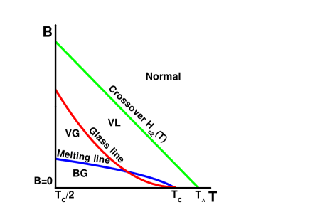
Figure 1: Magnetic phase diagram of high $T_{c}$ superconductors. VL is the vortex liquid region, while VG and BG are the vortex glass and Bragg glass.

The purpose of this note is to provide a convincing theoretical description of the magnetization data. Our conclusion is that the GL description of the layered materials $LSCO$, $BSCCO$ and $YBCO$ by the Lawrence - Doniach model within the self consistent fluctuation theory (SCFT, sometimes refered to as Hartree approximation) fits well the fluctuation effects in major families of HTSC materials in wide range of fields and temperatures and demonstrates that the fluctuation effects extend to well above $T_{c}$ far below $T^{\ast}$. This means that there is no evidence that the pseudogap physics influences the diamagnetism and that superconductivity probably plays no role at $T^{\ast}$.

Strong diamagnetism of a type II superconductor takes a form of network of Abrikosov flux lines (vortices) created by magnetic field. Vortices strongly interact with each other creating highly correlated configurations. A generic magnetic phase diagram of HTSC Li03 , Fig.1, contains four phases: two inhomogeneous phases, unpinned crystal and pinned Bragg glass and two homogeneous phases, unpinned vortex liquid and pinned vortex glass. In HTCS thermal fluctuations are strong enough to melt the lattices Zeldov95 into the vortex liquid over very large portion of the phase diagram. This portion covers the fields and temperatures of the above experiments, both above and below $T_{c}$ and for fields up to $40T$. The glass line separates pinned vortex matter (zero resistivity) from the unpinned one (nonzero resistivity due to flux flow).

Fluctuation diamagnetism in type II superconductors has been studied theoreticallyLarkin05 within both the microscopic theory (starting from the pioneering work of Aslamazov and Larkin) and the GL approach. In all of these calculations (with an exception of the strong field limit that allows the lowest Landau level approximation, see Li10 ) the fluctuations were assumed to be small enough, so they can be taken into account perturbatively. Within the GL approach this is referred to as the gaussian fluctuation theory (GFT)Larkin05 ; Carballeira00 . The GFT applied to the recent HTSC magnetization data was criticized Ong07 to fit just a single curve (magnetic field) rather than a significant portion of the magnetic phase diagram near $T_{c}$. To determine theoretically fluctuation diamagnetism for strong thermal fluctuations, one therefore must go beyond this simple approximation neglecting the effect of the quartic term in the GL free energy. The effect of the quartic term is taken into account within SCFT, widely used in physics of phase transitions at zero magnetic field and was adapted to transport property in magnetic field Dorsey91 ; Tinh09 . Since disorder is not considered, our results are limited to the vortex liquid phase of the magnetic phase diagram of Fig.1, where vortices are depinned.

The GL model of layered superconductor. Layered superconductor is sufficiently accurately described on the mesoscopic scale by the Lawrence-Doniach free energy (incorporating microscopic thermal fluctuation via dependence of parameters on temperature $T$, but not containing thermal fluctuations of the order parameter on the mesoscopic scale):

$$F\left[\psi\right] = s^{\prime}\sum_{l}\int_{\mathbf{r}}\left[\frac{\hbar^{2}}{2m_{a}}\left|\mathbf{D}\psi_{l}\right|^{2}+\frac{\hbar^{2}}{2m_{c}d^{\prime 2}}\left|\psi_{l}-\psi_{l+1}\right|^{2}\right.$$ (1)

$$\left.+\alpha\left(T-T_{\Lambda}\right)\left|\psi_{l}\right|^{2}+\frac{\beta}{2}\left|\psi_{l}\right|^{4}\right]\text{.}$$

Here $\psi_{l}\left(x,y\right)$ is the order parameter in the $l^{\text{th}}$ layer, $\mathbf{D\equiv\triangledown}+\frac{ie^{\ast}}{\hbar c}\mathbf{A}$, is the covariant derivative ($e^{\ast}=2|e|$) and $\mathbf{A}$ is the vector potential of magnetic field oriented along the crystallographic $c$ axis. The (effective) layer thickness is $s^{\prime}$ and the distance between the layers - $d^{\prime}$. Note that the temperature $T_{\Lambda}$, that will be called ”mean field” or ”bare” transition temperature, is larger than the real transition temperature $T_{c}$.

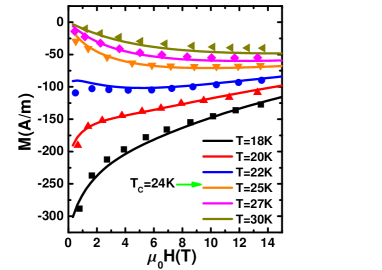
(a) LSCO

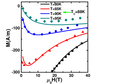
(b) BSCCO

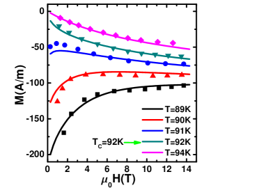
(c) YBCO

Figure 2: Magnetization data of ref.LuLi10 (dots) and their self consistent approximation fits (solid lines). Three major families of high $T_{c}$ superconductors are represented: (a) underdoped LSCO, (b) optimally doped BSCCO, (c) optimally doped YBCO. The curve closest to $T_{c}$ for each sample were used to determine the fitting parameters given in Table I. Each set of curves uses just three fitting parameters.

Table 1: Fitting parameters for LSCO, BSCCO, and YBCO.

$Material$	$T_{c}(Kelvin)$	$d^{\prime}({Angstrom})$	$H_{c2}(Tesla)$	$T_{\Lambda}(Kelvin)$	$\gamma$	$\Lambda$	$\kappa$	$Gi$
$LSCO$	$24$	$6.58$	$31$	$33$	$29$	$0.30$	66.7	$0.033$
$BSCCO$	$88$	$19.6$	$115$	$99$	$19$	$0.25$	55.6	$0.025$
$YBCO$	$92$	$11.68$	$220$	$100$	$4.1$	$0.22$	78.7	$0.0026$

The ”bare” coherence length $\xi=\hbar/\sqrt{2m_{a}\alpha T_{\Lambda}}$ will be used as the unit of length and the upper critical field $H_{c2}\equiv\hbar c/e^{\ast}\xi^{2}$ as the magnetic field unit. They depend on coarse graining scale (cutoff scale $\Lambda$) at which the mesoscopic model is derived (in principle) from The dimensionless order parameter is $\phi=\sqrt{\beta/2\alpha T_{\Lambda}}\psi$, so that the GL Boltzmann factor in scaled units takes a form,

$$f = \frac{F}{T}=\frac{1}{2\omega_{\Lambda}t_{\Lambda}}\sum_{l}\int_{\mathbf{r}}\left[\left|\mathbf{D}\phi_{l}\right|^{2}+d^{-2}\left|\phi_{l}-\phi_{l+1}\right|^{2}\right.$$ (2)

$$\left.-\left(1-t_{\Lambda}\right)\left|\phi_{l}\right|^{2}+\left|\phi_{l}\right|^{4}\right]\text{.}$$

Here $t_{\Lambda}=T/T_{\Lambda}$, $b=B/H_{c2}$ are dimensionless temperature and induction.It is more convenient to use the fluctuation strength parameter $\omega_{\Lambda}=\sqrt{2Gi_{\Lambda}}\pi/s$, instead of the more customary (”bare”) Ginzburg number $Gi_{\Lambda}=2\left(e^{\ast}/c\hbar\right)^{3}\kappa^{4}T_{\Lambda}^{2}\gamma^{2}/H_{c2}$. Since the renormalization by strong thermal fluctuations is central in this work, bare quantities carry index $\Lambda$, although the results used for fitting experiments will utilize renormalized parameters. The anisotropy $\gamma=\sqrt{m_{c}/m_{a}}$, $s=s^{\prime}\gamma/\xi_{\Lambda}$ and $d=d^{\prime}\gamma/\xi_{\Lambda}$. In strongly type II suprconductors the Ginzburg parameter $\kappa=\lambda/\xi>>1$ and magnetic field is nearly homogeneoussuppl , so we choose the Landau gauge $\mathbf{A}=(-by,0)$ in $\mathbf{D}=\mathbf{\nabla}+i\mathbf{A}$.

Fluctuation diamagnetism calculated within SCFT. The idea the method Li10 is as followssuppl . Let us divide the GL Boltzmann factor $f\left[\phi\right]$ into an optimized quadratic (”large”) part,

$$K = \frac{1}{2\omega_{\Lambda}t_{\Lambda}}\sum_{l}\int_{\mathbf{r}}\left[\left|\mathbf{D}\phi_{l}\right|^{2}+d^{-2}\left|\phi_{l}-\phi_{l+1}\right|^{2}\right.$$ (3)

$$\left.+\left(2\varepsilon-b\right)\left|\phi_{l}\right|^{2}\right]\text{,}$$

and a small perturbation

$$W=\frac{1}{2\omega_{\Lambda}t_{\Lambda}}\sum_{l}\int_{\mathbf{r}}\left[\left(t_{\Lambda}+b-1-2\varepsilon\right)\left|\phi_{l}\right|^{2}+\left|\phi_{l}\right|^{4}\right]\text{.}$$ (4)

Here, the variational parameter $\varepsilon$ (that depends on temperature, magnetic field and material parameters) has a physical meaning of the excitation gap in the vortex liquid phase. It is found from minimization of the variational free energy including the fluctuations on the mesoscopic scale. The only nontrivial technical difficulty is the summation over Landau levels in the presence of UV cutoff $\Lambda$. It is shownsuppl that to absorb all UV divergences one has to sum over Landau levels till the ”maximal” one $N_{\max}=\Lambda/b-1$. This results in the vortex liquid gap equation

$$\varepsilon = \frac{t_{\Lambda}+b-1}{2}+\frac{\omega_{\Lambda}t_{\Lambda}d}{2\pi^{2}}\int_{k=0}^{2\pi/d}\left\{\psi\left(g+\Lambda/b\right)-\psi\left(g\right)\right\};$$ (5)

$$g \equiv \left(1-\cos(kd)\right)/\left(d^{2}b\right)+\varepsilon/b\text{,}$$

where $\psi$ is the digamma function. The integration is over the Fourier harmonics $k$ in the $c$ direction.

The SCFT is widely used in GL model without magnetic field, $b=0$, under the name of ”mean field” and in this case simplifies to

$$\varepsilon = \left(t_{\Lambda}-1\right)/2+\omega_{\Lambda}t_{\Lambda}\left(h\left(\Lambda+\varepsilon\right)-h\left(\varepsilon\right)\right)\text{;}$$

$$h\left(u\right) = \ln\left(1+ud^{2}+\sqrt{2ud^{2}+\left(ud^{2}\right)^{2}}\right)/\pi\text{.}$$ (6)

In this case $\varepsilon$ has a meaning of the ”mass” of the field $\phi$ describing the fluctuations in the normal phase. It vanishes at the ”renormalized” transition temperature $T_{c}$ leading to its relation to $T_{\Lambda}$

$$T_{\Lambda}^{-1}=T_{c}^{-1}\left(1-2\omega h\left(\Lambda\right)\right)\text{.}$$ (7)

Here the renormalized coupling $\omega=\sqrt{2Gi}\pi/s$, this time expressed via renormalized Ginzburg number $Gi=2\left(e^{\ast}/c\hbar\right)^{3}\kappa^{4}T_{c}^{2}\gamma^{2}/H_{c2}$, is used. Expressing $T_{\Lambda}$ via $T_{c}$ in Eq.(5), the gap equation becomes,

$$\varepsilon = \frac{\omega td}{2\pi^{2}}\int_{k=0}^{2\pi/d}\left[\psi\left(g+\Lambda/b\right)-\psi\left(g\right)\right]$$ (8)

$$-\omega th\left(\Lambda\right)+\left(t+b-1\right)/2\text{,}$$

with $t=T/T_{c}$. Physical quantities are then calculated using numerical solution of this algebraic equation. For $b,\varepsilon<<\Lambda$ it is cutoff independent and simplifies:

$$\varepsilon=\left(t+b-1\right)/2-\frac{\omega td}{2\pi^{2}}\int_{k=0}^{2\pi/d}\left[\psi\left(g\right)+\ln 2\right]\text{.}$$ (9)

Magnetization issuppl ,

$$M=\frac{\omega stH_{c2}}{8\pi^{3}\kappa^{2}}\int_{k=0}^{2\pi/d}\left[\left(g+\Lambda/b-1/2\right)\psi\left(g+\Lambda/b\right)\right.$$

$$\left.-\left(g-1/2\right)\psi\left(g\right)+\ln\left(\Gamma\left(g\right)/\Gamma\left(g+\Lambda/b\right)\right)-\Lambda/b\right]\text{,}$$ (10)

while for $b,\varepsilon<<\Lambda$ it simplifies to

$$M=\frac{\omega stH_{c2}}{8\pi^{3}\kappa^{2}}\int_{k=0}^{2\pi/d}\left[\ln\frac{\Gamma\left(g\right)}{\sqrt{2\pi}}+g-\left(g-\frac{1}{2}\right)\psi\left(g\right)\right]\text{.}$$ (11)

In certain portions of the magnetic phase diagrams the strong inequalities $b,\varepsilon<<\Lambda$ are not obeyed, while SCFT is still valid, so we have used the formula Eq.(10), with weak (logarithmic) cutoff dependence instead of the cutoff independent renormalized formula.

Comparing with experiments and GFT. Recent accurate magnetization data LuLi10 on magnetization of three major families of HTSC materials, including underdoped $La_{2-x}Sr_{x}CuO_{4}$ for $x=0.09$, optimally doped $Bi_{2}Sr_{2}CaCu_{2}O_{8+\delta}$, and optimally doped $YBa_{2}Cu_{3}O_{7}$, are fitted in Fig. 2a, 2b, 2c respectively. Measured magnetization curves of $LSCO$ and $YBCO$ in the $0-14T$ field range and $BSCCO$ at $0-40T$ show distinct features above and below $T_{c}$, thus allowing meaningful fitting. The conditions $b,\varepsilon<<\Lambda$ are obeyed provided temperature does not deviate too far from $T_{c}$ and magnetic field is small compared to $H_{c2}$. Several temperatures within $10\%$ of $T_{c}$ were used to determine three fitting parameters, $H_{c2}$, anisotropy $\gamma$, and $\kappa^{2}/s$, using simplified formulas Eqs.(9, 11). The interlayer distances $d^{\prime}$ were taken from Poole2007 . Near $T_{c}$, the correlation length is large, therefore we take $s=d$, as the maximum value of $s$. The results for each material are given in Table I.

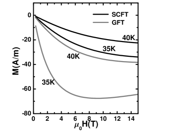
Figure 3: The comparison between the fluctuation magnetization of $LSCO$ calculated using the self consistent fluctuation theory (SCFT) vs the perturbative gaussian fluctuation (GFT) one.

For the rest of the data (higher temperature and higher magnetic field) the theoretical curves shown in Fig. 2. were logarithmically dependent on cutoff and therefore the full formulas, Eqs.(5, 10), were utilized. The two additional parameters, namely mean field critical temperature $T_{\Lambda}$ and $\Lambda$ are constrained via Eq.(7) (with experimentally measured $T_{c}$ also listed in Table I). The values of $T_{\Lambda}$ and $\Lambda$ in units of $\hbar e^{\ast}H_{c2}/(m_{a}c)$ are given in Table I.

To demonstrate the importance of nonperturbative effects the SCFT magnetization, Eq.(10) is compared with GFT within the 2D layered superconductors model Carballeira00 in Fig. 3. One observes that The SCFT magnitude is much smaller than the GFT one. One of the reasons is that the vortex liquid gap $\varepsilon$ is larger than the reduced temperature (perturbative gap) $\left(t_{\Lambda}+b-1\right)/2$.

The data of ref. LuLi10 in the region of smaller fields exhibit the so called ”intersection point” of the magnetization curves plotted as function of temperature. Our magnetization curves (underdoped $LSCO$ is shown in Fig. 4 as an example) demonstrate the intersection point in this region for all three materials. The intersection points were measured in many high $T_{c}$ cuprate Salem and explained within the ”lowest Landau level” approximation Lin05 valid for $\varepsilon<<b$. It turns out that an addition requirement for the intersection point is $\varepsilon d^{2}>>1$. Our results demonstrate that beyond this approximation the intersection point disappears.

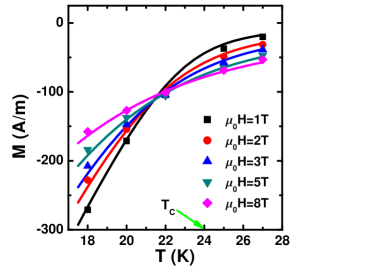
Figure 4: Fit of magnetization LuLi10 in the region of the intersection point (fields lower than those shown in Fig. 2a) in LSCO using the same fitting parameters (given in Table I).

Conclusions. We have investigated the fluctuation diamagnetism of HTSC using a self consistent nonperturbative method beyond gaussian fluctuations term within Lawrence - Doniach GL model. The comparison with recent accurate experiments near $T_{c}$ demonstrate that the effect of quartic terms should to be included due to strong fluctuations. The theory describes well wide class of materials from relatively low anisotropy optimally doped $YBCO$ to highly anisotropic underdoped $LSCO$ and optimally doped $BSCCO$ at temperatures both below and above $T_{c}$. No input from the microscopic ”pseudogap” physics is needed to describe the magnetization data. Dynamical effects like Nernst effect, electrical and thermal conductivity can be in principle approached within the similar SCFT generalized to a time dependent variants of the GL model.

- (1) T. Timusk and B. Statt, Rep. Prog. Phys. 62, 61 (1999).
- (2) V. J. Emery and S. A. Kivelson, Nature 374, 434 (1995); P. A. Lee and X. G. Wen, Phys. Rev. Lett. 78, 4111 (1997); A. Levchenko, M. R. Norman, and A. A. Varlamov, Phys. Rev. B 83, 020506 (2011).
- (3) Z. A. Xu, N. P. Ong, Y. Wang, T. Kakeshita and S. Uchida, Nature 406, 486 (2000); Y. Wang, Z. A. Xu, T. Kakeshita, S. Uchida, S. Ono, Yoichi Ando, and N. P. Ong, Phys. Rev. B 64, 224519 (2001); Y. Wang, N. P. Ong, Z. A. Xu, T. Kakeshita, S. Uchida, D. A. Bonn, R. Liang, and W. N. Hardy, Phys. Rev. Lett. 88, 257003 (2002).
- (4) Y. Wang, Lu Li, and N. P. Ong, Phys. Rev. B 73, 024510 (2006).
- (5) F. Rullier-Albenque, H. Alloul, and G. Rikken, Phys. Rev. B 84, 014522 (2011) and references therein; M. S. Grbic, M. Pozek, D. Paar, V. Hinkov, M. Raichle, D. Haug, B. Keimer, N. Barisic, and A. Dulcic, Phys. Rev. B 83, 144508 (2011).
- (6) K. Kudo, M. Yamazaki, T. Kawamata, T. Adachi, T. Noji, Y. Koike, T. Nishizaki, and N. Kobayashi, Phys. Rev. B 70, 014503 (2004).
- (7) Lu Li, Y. Wang, S. Komiya, S. Ono, Y. Ando, G. D. Gu, and N. P. Ong, Phys. Rev. B 81, 054510 (2010); Y. Wang, Lu Li, M. J. Naughton, G. D. Gu, S. Uchida, and N. P. Ong, Phys. Rev. Lett. 95, 247002 (2005).
- (8) A. Larkin and A. Varlamov, Theory of fluctuations in superconductors, (Clarendon Press, Oxford, 2005).
- (9) J. Chang, N. Doiron-Leyraud, O. Cyr-Choini re, G. Grissonnanche, F. Lalibert , E. Hassinger, J-Ph. Reid, R. Daou, S. Pyon, T. Takayama, H. Takagi, and Louis Taillefer, Nature Phys. 8, 751 (2012).
- (10) I. Ussishkin, S. L. Sondhi, and D. A. Huse, Phys. Rev. Lett. 89, 287001 (2002); A. Sergeev, M. Y. Reizer, and V. Mitin, Phys. Rev. B 77, 064501 (2008); Phys. Rev. Lett. 106, 139701 (2011); M. N. Serbyn, M. A. Skvortsov, A. A. Varlamov, and V. Galitski, Phys. Rev. Lett. 102, 067001 (2009); Phys. Rev. Lett. 106, 139702 (2011).
- (11) S. A. Kivelson and E. H. Fradkin, Physics 3, 15 (2010).
- (12) D. Li and B. Rosenstein, Phys. Rev. Lett. 90, 167004 (2003); Phys. Rev. B 70, 144521 (2004); Beidenkopf, T. Verdene, Y. Myasoedov, H. Shtrikman, E. Zeldov, B. Rosenstein, D. Li, and T. Tamegai, Phys. Rev. Lett. 98, 167004 (2007).
- (13) E. Zeldov, D. Majer, M. Konczykowski, V. B. Geshkenbein, V. M. Vinokur, and H. Shtrikman, Nature 375, 373 (1995).
- (14) B. Rosenstein and D. Li, Rev. Mod. Phys. 82, 109 (2010).
- (15) R. E. Prange, Phys. Rev. B 1, 2349 (1970); C. Carballeira, J. Mosqueira, A. Revcolevschi, and F. Vidal, Phys. Rev. Lett. 84 3157 (2000); Physica C 384 185 (2003); A. Lascialfari, A. Rigamonti, L. Romano, A. A. Varlamov, and I. Zucca, Phys. Rev. B 68, 100505 (2003).
- (16) L. Cabo, J. Mosqueira, and F. Vidal, Phys. Rev. Lett. 98, 119701 (2007); N. P. Ong, Y. Wang, Lu Li, and M. J. Naughton, Phys. Rev. Lett. 98, 119702 (2007).
- (17) S. Ullah and A. T. Dorsey, Phys. Rev. B 44, 262 (1991).
- (18) B. D. Tinh and B. Rosenstein, Phys. Rev. B 79, 024518 (2009); B. D. Tinh, D. Li, and B. Rosenstein, Phys. Rev. B 81 224521 (2010).
- (19) See Supplemental Material for further details.
- (20) C. P. Poole Jr., H. A. Farach, R. J. Creswick, and R. Prozorov, Superconductivity (Academic Press, Amsterdam, 2007).
- (21) S. Salem-Sugui, Jr., J. Mosqueira, and A. D. Alvarenga, Phys. Rev. B 80, 094520 (2009); S. Salem-Sugui Jr., A. D. Alvarenga, J. Mosqueira, J. D. Dancausa, C. Salazar Mejia, E. Sinnecker1, H. Luo and H. Wen, Supercond. Sci. Technol. 25. 105004 (2012); J. Mosqueira, L. Cabo, and F. Vidal, Phys. Rev. B 76, 064521 (2007); B. Rosenstein, B. Ya. Shapiro, R. Prozorov, A. Shaulov, and Y. Yeshurun, Phys. Rev. B 63, 134501 (2001); Y. M. Huh and D. K. Finnemore, Phys. Rev. B 65, 092506 (2002); M. J. Naughton, Phys. Rev. B 61, 1605 (2000).
- (22) Z. Tesanovic, L. Xing, L. Bulaevskii, Q. Li, and M. Suenaga, Phys. Rev. Lett. 69, 3563 (1992); F. P. Lin and B. Rosenstein, Phys. Rev. B 71, 172504 (2005).