Blueberryrgb0.25,0,0.65 \definecolorStrawberryrgb0.65,0,0.25
‘
Holographic turbulence
Abstract
We construct turbulent black holes in asymptotically AdS4 spacetime by numerically solving Einstein equations. Both the dual holographic fluid and bulk geometry display signatures of an inverse cascade with the bulk geometry being well approximated by the fluid/gravity gradient expansion. We argue that statistically steady-state black holes dual to dimensional turbulent flows have horizons which are approximately fractal with fractal dimension .
Introduction.—According to holography, turbulent flows in relativistic boundary conformal field theories should be dual to dynamical black hole solutions in asymptotically AdSd+2 spacetime with the number of spatial dimensions the turbulent flow lives in. This immediately raises many interesting questions about gravitational dynamics. For example, what distinguishes turbulent black holes from non-turbulent ones? What is the gravitational origin of energy cascades and the Kolmogorov scaling observed in turbulent fluid flows?
Gravitational dynamics can also provide insight into turbulence itself. This is particularly relevant for problems where physics beyond hydrodynamics may play a crucial role in turbulent evolution, since holography provides a complete description of physics valid on all length scales. For superfluid turbulence, where vortex dynamics and turbulent evolution are not governed by hydrodynamics, holography has already yielded valuable insight and demonstrated two dimensional holographic superfluids can exhibit a direct energy cascade to the UV Adams et al. (2012). Likewise, having control of regimes beyond the hydrodynamic description of turbulence of normal fluids may allow one to study the domain of validity and the late-time regularity of solutions to the Navier-Stokes equation.
In this paper we take a first step towards studying holographic turbulence by numerically constructing black hole solutions in asymptotically AdS4 spacetime dual to turbulent flows, where energy flows from the UV to the IR in an inverse cascade. We propose a simple geometric measure to distinguish turbulent black holes from non-turbulent ones: the horizon of a turbulent black hole exhibits a fractal-like structure with effective fractal dimension . The in this formula can be understood as the geometric counterpart of the rapid entropy growth implied by the Kolmogorov scaling.
Numerics and Gravitational Description.—We generate turbulent evolution by numerically solving Einstein’s equations
| (1) |
with cosmological constant . Our numerical scheme for solving Einstein’s equations is outlined in Chesler and Yaffe (2011, 2009); Cardoso et al. (2012) and will be further elaborated on in a coming paper Chesler and Yaffe (To appear shortly). In what follows we focus on some of the salient details.
We employ a characteristic formulation of Einstein’s equations and choose the metric ansatz
| (2) |
with Greek indices running over the boundary spacetime coordinates. The coordinate is the AdS radial coordinate with corresponding the the AdS boundary. The metric ansatz (2) is invariant under the residual diffeomorphism for arbitrary . Since the geometry we study contains a black brane with planar topology, we fix the residual diffeomorphism invariance by demanding the apparent horizon be at . Horizon excision is then performed by restricting the computational domain to .
The AdS boundary is causal and therefore boundary conditions must be imposed there. Solving Einstein’s equations with a series expansion about , one finds an asymptotic expansion of the form . All omitted terms in the expansion are determined by and and their derivatives. The expansion coefficient corresponds to the metric the dual turbulent flow lives in. Hence we choose the boundary condition . The expansion coefficient is determined by solving Einstein’s equations and encodes the expectation value of the boundary stress tensor de Haro et al. (2001)
| (3) |
where is Newton’s constant.
We choose initial data corresponding to a locally boosted black brane with metric 111 In the characteristic formulation of Einstein’s equations sufficient initial data consists of the conserved boundary densities and the rescaled spatial metric Cardoso et al. (2012); Chesler and Yaffe (To appear shortly). With these quantities specified at all other components of the metric can be determined by solving Einstein’s equations Cardoso et al. (2012); Chesler and Yaffe (To appear shortly). Therefore, when using (4) as initial data we only use and .
| (4) |
where is the local boost velocity and with the local temperature of the brane. The function satisfies
We work in a periodic spatial box of size . We choose the initial boost velocity
| (5) |
with . The small fluctuations are present to break the symmetry of the initial conditions. We choose to be a sum of the first four spatial Fourier modes with random coefficients and phases and adjust the overall amplitude of such that . These initial conditions are unstable and capable of producing subsequent turbulent evolution if the Reynolds number is sufficiently large. For our initial conditions . We choose box size and the initial temperature .
We discretize Einstein’s equations using pseudospectral methods and represent the radial dependence of all functions in terms of an expansion of Chebyshev polynomials and the dependence of all functions in terms of an expansion of plane waves. We then evolve the discretized geometry for 3001 units of time.
Results and Discussion.—To illustrate the turbulent flow generated by solving Einstein’s equations in Fig. 1 we plot of the boundary vorticity at three different times. To compute the vorticity we first extract the boundary stress tensor from the metric via Eq. (3). We then define the fluid velocity as the normalized future-directed time-like eigenvector of ,
| (6) |
with the proper energy density.
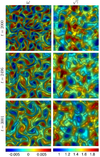
During times through our system experiences an instability which drives our initial state into turbulent evolution. At all times shown in Fig. 1 there is little sign of the initial sinusoidal structure present in the initial data (5). At time there are many vortices present with fluid rotating clockwise (red) and counterclockwise (blue). During the latter evolution seen at times and isolated vortices with the same rotation tend to merge together to produce larger and larger vortices. The merging of vortices of like-rotation to produce larger vortices is a tell tale signature of an inverse cascade.
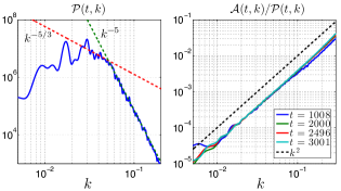
It is interesting to compare our results to the Kolmogorov theory of turbulence. A classic result from Kolmogorov’s theory is that for driven steady-state turbulence the power spectrum of the fluid velocity,
| (7) |
with , obeys the scaling
| (8) |
in an inertial range . Despite the fact that our system is not driven or in a steady-state configuration we do see hints of the Kolmogorov scaling. In Fig. 2 we plot at time . Our numerical results are consistent with the scaling (8) in the inertial range . As we are not driving the system, evidence of the scaling is transient and destroyed first in the UV, with the UV knee at shifting to the IR as time progresses. Beyond the inertial range the spectrum decreases like with until . We comment further below on the UV behavior of .
The inverse cascade also manifests itself in gravitational quantities. One interesting quantity to consider is the horizon area element . In our coordinate system and in the limit of large Reynolds number the event and apparent horizons approximately coincide at and the horizon area element is 222 In the fluid/gravity gradient expansion the apparent and event horizons coincide up to second order in gradients. Hence their positions should coincide in the limit. . Also included in Fig. 1 are plots of . At exhibits structure over a large hierarchy of scales and is fractal-like in appearance. We comment more on this further below. However, as time progresses becomes smoother and smoother just as the fluid vorticity does due to the inverse cascade.
The velocity power spectrum also imprints itself in bulk quantities. One quantity to consider is the extrinsic curvature of the event horizon. can be constructed from the null normal to the horizon and an auxiliary null vector whose normalization is conveniently chosen to satisfy . The extrinsic curvature is then given by with . Since the horizon is at we choose and . The horizon curvature satisfies where run over the spatial coordinates. For later connivence we define the rescaled traceless horizon curvature where is the traceless part of the extrinsic curvature and is defined by the geodesic equation .
Also included in Fig. 2 are plots of where the horizon curvature power spectrum is
| (9) |
with . As Fig. 2 makes clear, our numerical results are consistent with
| (10) |
Evidently, bulk quantities — even at the horizon — are correlated with boundary quantities. As we detail below, this is a consequence of the applicability of the fluid/gravity correspondence.
Both qualitative and quantitative aspects of our results can be understood in terms of relativistic conformal hydrodynamics and the fluid/gravity correspondence. In the limit of asymptotically slowly varying fields (compared to the dissipative scale set by the local temperature of the system) Einstein’s equations (1) can be solved perturbatively with a gradient expansion where is order in boundary spacetime derivatives Bhattacharyya et al. (2008). The expansion coefficients can be expressed in terms of the boundary quantities and and their spacetime derivatives. The leading order term is just the locally boosted black brane (4). Likewise, via Eq. (3) the bulk gradient expansion encodes the boundary stress gradient expansion . The expansion coefficient is the stress tensor of ideal conformal hydrodynamics. Likewise, is the viscous stress tensor of conformal hydrodynamics with the shear viscosity and the shear tensor given below in (15). The underlying evolution of and and hence the bulk geometry is governed by conservation of the boundary stress tensor. Hence at leading order in gradients the evolution of and is governed by ideal relativistic hydrodynamics and the geometry is given by the boosted black brane metric (4). Indeed, it was recently demonstrated in Carrasco et al. (2012) that turbulence in ideal conformal relativistic hydrodynamics gives rise to an inverse cascade and exhibits the Kolmogorov scaling (8).
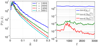
Our first hint of the applicability of the fluid/gravity gradient expansion comes from studying the power spectrum of the fluid velocity at high and the relative importance of viscous effects. In Fig. 3 we plot at for different times on a semi-log scale. As shown in the figure, our results are consistent with exponential decay of for with . With our choice of units where , the kinematic viscosity . Therefore, at the scale viscous effects are suppressed by an order ten factor relative to inertial effects. This suggest that the hydrodynamic gradient expansion on the boundary is well behaved.
Likewise, we find that our numerical metric is very well approximated by the fluid/gravity gradient expansion. To perform the comparison, via Eq. (6) we extract and (and hence ) from . We then use and to construct the expansion functions computed in Van Raamsdonk (2008). We then take the difference and define the order error to be at each time . As shown in Fig. 3, the boosted black brane metric (4) approximates the geometry at the 1% level. Including first order gradient corrections further decreases the size of the error 333 Near time , when the size of the first order corrections to the metric is comparable to the truncation error of our numerical calculation. In particular, by monitoring the validity of temporal constraint equations we can ascertain the degree of convergence of our numerics. Near time the constraints are satisfied at order 1 part in which is the same size as the first order gradient correction to the geometry. The degree in which the constraints are satisfied can be improved by decreasing the spatial grid spacing. We suspect that using a finer resolution will decrease .
It is natural that turbulent evolution gives rise to dual geometries well approximated by locally boosted black branes. First of all, irrespective of turbulent flows require Reynolds number , or equivalently, very small gradients compared to . This is precisely the regime where the gradient expansions of fluid/gravity should be well behaved. Second, the inverse cascade of turbulence implies that gradients become smaller and smaller as energy cascades from the UV to the IR. Therefore, the leading term (4) should become a better and better approximation to the metric as time progresses and the inverse cascade develops.
At least for the above observation has powerful consequences for studying turbulent black holes. Instead of numerically solving the equations of general relativity one can simply study the equations of hydrodynamics and construct the bulk geometry via the fluid/gravity gradient expansion. This is particularly illuminating in the limit of non-relativistic fluid velocities , where the bulk geometry and boundary stress are asymptotically close to equilibrium. As shown in Bhattacharyya et al. (2009), under the rescalings with the variation in the temperature away from equilibrium, in the limit the boundary evolution of and implied by the fluid/gravity correspondence reduces to the non-relativistic incompressible Navier-Stokes equation. Indeed, the above rescalings are symmetries of the Navier-Stokes equation. Likewise, in the limit the geometry dual to the Navier-Stokes equation is encoded in the expansion functions and which are known analytically Bhattacharyya et al. (2008); Van Raamsdonk (2008). At least for , where is it well known that solutions to the Navier-Stokes equation are stable, we therefore expect many known results from classic studies of turbulence – such as the Kolmogorov scaling (8) – to carry over naturally and semi-analytically to gravity.
As an illustration of the above point we now turn our attention to the horizon of turbulent black holes and argue that the Kolmogorov scaling (8) together with the relation (10) implies that the turbulent horizons are fractal-like in nature with non-interger fractal dimension. To augment our numerical evidence of (8) and (10) we assume the validity of the fluid/gravity gradient expansion for any and that the system is driven by an external force into a statistically steady-state configuration and that the Kolmogorov scaling applies over an arbitrarily large and static inertial range. Within the gravitational description the driving can be accomplished by a time-dependent deformation of the boundary geometry Chesler and Yaffe (2009); Bhattacharyya et al. (2009).
The fractal dimension of the horizon can be extracted from the horizon area. Introducing a spatial regular , one could compute the horizon area via the Riemann sum where each element . The fractal dimension is defined by the scaling
| (11) |
in the limit.
To see how the Kolmogorov scaling (8) implies the horizon has a fractal structure we employ the Raychaudhuri equation,
| (12) |
which relates the change in the horizon’s area element to the traceless part of horizon’s extrinsic curvature 444 For a review of this topic see Gourgoulhon and Jaramillo (2006)) . Here is the Lie derivative with respect to the null normal to the horizon and . In the hydrodynamic limit of slowly varying fields salient to turbulent flows the Raychaudhuri equation simplifies to Integrating over the horizon, it follows that the rate of change of the horizon area is
| (13) |
where is given in (9). We therefore see that encodes the growth of the horizon area.
Using the locally boosted black brane metric (4), can be computed as a gradient expansion. For geometries dual to fluid flows in spatial dimensions the leading order results read Eling and Oz (2010)
| (14) |
with and
| (15) |
We note that is orthogonal to the fluid velocity and traceless . Using (9) and (14) we see that at leading order in gradients is the power spectrum of . Counting derivatives we therefore see that (10) must be satisfied at leading order in gradients, just as demonstrated in Fig. 2.
Assuming that the system is driven into a steady-state and the Kolmogorov scaling (8) applies, from (10) we see that for any we have . Inserting a UV regulator into the momentum integral in (13) at we conclude that for
| (16) |
Integrating and identifying we conclude from (11) that the fractal dimension of the horizon is
| (17) |
We note, however, that the scaling (11) is never exactly obtained for a turbulent horizon. The UV terminus of the inertial range is bounded by the dissipative scale , where hydrodynamics breaks down. Hence the scaling (16) can apply no further than . However, the constant of integration one gets from integrating (16) is of order , which is the area element of an equilibrium black brane. Hence the scaling of the horizon area never dominates over the constant and the scaling (11) is never exactly satisfied in the large limit. However, the domain in which the scaling (16) applies can be made arbitrarily large as is bounded only by the system size. Therefore, what Eqs. (16) and (17) encode is that turbulent horizons have geometric features over a large hierarchy of scales, just as seen in the plots of in Fig. 1.
The origin of the fractal-like structure of the horizon is easy to understand. It is well known from fluid mechanics that turbulent flows have a fractal-like structure with large vortices being composed of smaller vortices which are themselves composed of smaller vortices and so on. This behavior can be seen in the plots of the vorticity in Fig. 1. Via the fluid/gravity gradient expansions this fractal-like structure imprints itself on the bulk geometry. Moreover, upon using Hawking’s formula to relate the horizon area to entropy, the Raychaudhuri equation (13) combined with (14) translates into the familiar expression for entropy growth in hydrodynamics with the shear viscosity of the fluid (which for theories with gravitational duals is given by with the proper entropy density Kovtun et al. (2005)) Eling and Oz (2010). Thus the fractal horizon can be understood as the geometric counterpart of the familiar fact that turbulent flows generate entropy much more rapidly than laminar flows with the same rate of energy dissipation.
We conclude by discussing the origin of the inverse cascade for . It is well known that the inviscid Navier-Stokes equation conserves the enstrophy and that conservation of enstrophy necessitates and inverse cascade. Moreover, it has recently been demonstrated that the equations of ideal relativistic conformal hydrodynamics salient to holographic turbulence conserve the relativistic generalization of the enstrophy
| (18) |
Carrasco et al. (2012). Conservation of in hydrodynamics suggests that there should exist an analogous conserved quantity in the gravitational description which is also only conserved for . Since the enstrophy is constructed from the vorticity , a natural starting point is finding a gravitational quantity which encodes . As is a pseudoscalar in two spatial dimensions a natural guess is the gravitational Pontryagin density . With this guess we define the gravitational enstrophy 555 We note there are other gravitational quantities that encode both the vorticity and enstrophy.
| (19) |
where the integration is over the horizon. Using the boosted black brane metric (4) and expanding in powers of derivatives we find Hence up to a numerical factor coincides with the fluid enstrophy . Evidently, in the long wavelength limit evolution generated by Einstein’s equations must conserved .
Acknowledgements.
Acknowledgments.—We acknowledge helpful conversations with Christopher Herzog, Veronika Hubeny, Luis Lehner, Mukund Rangamani, and Laurence Yaffe. AA thanks the Aspen Center for Physics for hospitality. The work of AA is supported in part by the U.S. Department of Energy (D.O.E.) under cooperative research agreement #DE-FC02- 94ER40818. The work of PC is supported by a Pappalardo Fellowship in Physics at MIT. The work of HL is partially supported by a Simons Fellowship and by the U.S. Department of Energy (D.O.E.) under cooperative research agreement #DE-FG0205ER41360.References
- Adams et al. (2012) A. Adams, P. M. Chesler, and H. Liu, Science 341, 368 (2012), eprint 1212.0281.
- Chesler and Yaffe (2011) P. M. Chesler and L. G. Yaffe, Phys.Rev.Lett. 106, 021601 (2011), eprint 1011.3562.
- Chesler and Yaffe (2009) P. M. Chesler and L. G. Yaffe, Phys.Rev.Lett. 102, 211601 (2009), eprint 0812.2053.
- Cardoso et al. (2012) V. Cardoso, L. Gualtieri, C. Herdeiro, U. Sperhake, P. M. Chesler, et al., Class.Quant.Grav. 29, 244001 (2012), eprint 1201.5118.
- Chesler and Yaffe (To appear shortly) P. M. Chesler and L. G. Yaffe (To appear shortly).
- de Haro et al. (2001) S. de Haro, S. N. Solodukhin, and K. Skenderis, Commun.Math.Phys. 217, 595 (2001), eprint hep-th/0002230.
- Bhattacharyya et al. (2008) S. Bhattacharyya, V. E. Hubeny, S. Minwalla, and M. Rangamani, JHEP 0802, 045 (2008), eprint 0712.2456.
- Carrasco et al. (2012) F. Carrasco, L. Lehner, R. C. Myers, O. Reula, and A. Singh, Phys.Rev. D86, 126006 (2012), eprint 1210.6702.
- Van Raamsdonk (2008) M. Van Raamsdonk, JHEP 0805, 106 (2008), eprint 0802.3224.
- Bhattacharyya et al. (2009) S. Bhattacharyya, S. Minwalla, and S. R. Wadia, JHEP 0908, 059 (2009), eprint 0810.1545.
- Eling and Oz (2010) C. Eling and Y. Oz, JHEP 1002, 069 (2010), eprint 0906.4999.
- Kovtun et al. (2005) P. Kovtun, D. Son, and A. Starinets, Phys.Rev.Lett. 94, 111601 (2005), eprint hep-th/0405231.
- Gourgoulhon and Jaramillo (2006) E. Gourgoulhon and J. L. Jaramillo, Phys.Rept. 423, 159 (2006), eprint gr-qc/0503113.