The Power of Spreadsheet Computations

We investigate the expressive power of spreadsheets. We consider spreadsheets which contain only formulas, and assume that they are small templates, which can be filled to a larger area of the grid to process input data of variable size. Therefore we can compare them to well-known machine models of computation. We consider a number of classes of spreadsheets defined by restrictions on their reference structure. Two of the classes correspond closely to parallel complexity classes: we prove a direct correspondence between the dimensions of the spreadsheet and amount of hardware and time used by a parallel computer to compute the same function. As a tool, we produce spreadsheets which are universal in these classes, i.e. can emulate any other spreadsheet from them. In other cases we implement in the spreadsheets in question instances of a polynomial-time complete problem, which indicates that the the spreadsheets are unlikely to have efficient parallel evaluation algorithms. Thus we get a picture how the computational power of spreadsheets depends on their dimensions and structure of references.

1 Introduction

1.1 Why spreadsheets?

Spreadsheets are an extremely popular type of software systems. They have conquered very diverse areas of present day politics, business, research, and, last but not least, our private lives. However, this prevalence is not so evident, because spreadsheets are typically used in the back office and are not presented to the public. They make to the news only when something went really wrong: for instance a spreadsheet used to justify a widely implemented public policy, as in the case of the extremely influential report [11] concerning a supposed causal relationship between high national debt and low economic growth, turns out to contain an error in a formula, affecting the outcome of the calculations [7]. Or when an Excel model was used to manage the investments of JPMorgan Chase & Co. bank, which led to trade losses estimated in billions of dollars [8]. Research is not an exception, and a careful reader of Science magazine can read [6, 2], in which a scientific controversy finally turns out to be related to a spreadsheet mistake.

Indeed, spreadsheets are among the most frequently used software tools of any kind. Despite that, and surprisingly enough, very little has been known about their computational power. Consequently, the users are not really aware of the abilities and limitations of the tool they use.

1.2 How to measure expressiveness of spreadsheets

The aim of this paper is to analyze the power of spreadsheets considered as a tool for specifying general-purpose computations.

It is clear that they belong to the nonuniform computation models, where for each input size there is a separate computing device. Uniformity can be introduced to such a model by imposing that there is a common, low complexity procedure to create those devices, given the input size. In this respect, spreadsheets come with a natural, built-in solution of this issue: filling, i.e. automated copying of formulas into neighboring cells, with suitable reference adjustments. In spreadsheet programming practice, filling is the usual way to produce a spreadsheet processing a large amount of data from a few formulas prepared manually, or to adjust an already existing one to accommodate a new supply of data.

We follow this idea and treat a small spreadsheet consisting of a few initial cells with formulas as a program, and filling as a method to run it on input data of variable size. The input data is also located in the spreadsheet, but is not subject to filling. For mathematical convenience, we imagine that the spreadsheet grid is actually infinite and any number of rows and columns can be filled with copies of the initial cells. These two assumptions allow us to apply the methods of computational complexity, which are asymptotic in nature, to the study of spreadsheets.

No macros and user-defined functions written in a general programming language are permitted. A few specific and infrequently occurring spreadsheet functions are also excluded from our analysis.

1.3 Main results

The structural properties of spreadsheets which determine their computational properties are defined by restrictions on the pattern of references of formulas to other cells and do not apply to the references to input data:

1. A spreadsheet is row-organized if all ranges to which its formulas refer are horizontal ones, i.e., rows.

2. A spreadsheet is row-directed if every formula refers only to cells and ranges located strictly above the location of the formula itself.

These properties are preserved by filling. Our findings described below refer also to the analogous column-organized and column-directed spreadsheets. Thus we get several possible combinations of column-related and row-related properties.

We describe the computational power of spreadsheets by relating them to Parallel Random Access Machines (PRAM for short).

We encounter both Concurrent Read Concurrent Write (CRCW) priority write machines and Exclusive Read Exclusive Write (EREW) ones.

On several occasions we proceed by implementing instances of the $P$-complete Circuit Value Problem (abbreviated CVP) in spreadsheets, in order to demonstrate that they are unlikely to have efficient parallel evaluation algorithms.

Our first main result is that any given initial row-organized row-directed spreadsheet can be converted into a program $\pi$ for an EREW PRAM such that the function computed by that spreadsheet filled to the dimensions of $c$ columns and $r$ rows is always the same as that computed by $\pi$ evaluated on a PRAM with $c$ processors, $O(c)$ cells of memory and running for $O(r\log c)$ time. Thus, if a spreadsheet is row-organized row-directed, it can be efficiently parallelized: its number of columns contributes only a logarithmic factor to the total computation time. This sets an upper bound on the computational power of row-organized row-directed spreadsheets. An analogous result holds for column-organized column-directed spreadsheets.

In order to get a lower bound, and thus determine the class of functions computable by those spreadsheets, we prove our second main result: there is a row-organized row-directed spreadsheet with 19 formulas which is a universal CRCW PRAM evaluator, i.e., one which given a (suitably encoded) program $\pi$ together with its input, and filled to the dimensions of $p$ columns and $10t$ rows, computes in its last row the description of PRAM after executing $t$ steps of $\pi$ on $p$ processors and with $p$ cells of shared memory. This demonstrates that spreadsheets can implement a natural and broad class of general-purpose computations.

This spreadsheet is also a universal row-organized row-directed spreadsheet: any other spreadsheet from this class can be equivalently expressed as a program for a PRAM, which in turn can be executed on that spreadsheet. This above results demonstrate that row-organized row-directed spreadsheets and PRAMs are almost equivalent in computing power, with clear relations between the resources in both models. Indeed, translating a spreadsheet into an equivalent program for PRAM, and then back to spreadsheet, incurs only a logarithmic overhead, a common effect of translations between different parallel computation models.

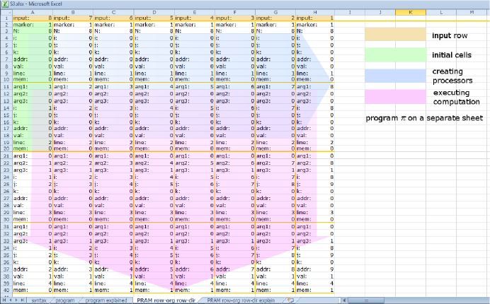
Figure 1: PRAM evaluator in a row-organized row-directed spreadsheet S1: structure and mode of operation. Processors are located in columns, and computation time advances downwards. A vertical group of 10 cells constitutes a snapshot of a processor at a given time, so that extending computation time by one unit requires filling 10 rows. It is provided as an electronic appendix S1.

At the same time PRAMs and spreadsheets are extremely different: the former have only programming primitives and no data analysis ones, while the latter have only data analysis functions and do not support any form of programming on the level of the spreadsheet itself.

Our result indicates that it is possible and feasible to turn row-organized row-directed spreadsheets into a potential programming language for specifying general-purpose parallel computations, with clear relation between the dimensions of the spreadsheet and complexity of its formulas, and the computational resources necessary to execute it. They might be particularly dedicated for users who have high computing needs but no programming training.

Let us move to other classes of spreadsheets, not necessarily row-oriented ones. We demonstrate a row-organized but not row-oriented PRAM simulator (electronic appendix S2), more powerful than the one previously described. If it is extended to $c$ columns and $r$ rows, computes the description of PRAM after executing $cr/10p$ steps of $\pi$ on $p$ processors and with $p$ cells of shared memory, where $p\leq c$ is a part of the input. Thus this PRAM simulator can perform a parallel or a sequential computation, depending on the actual input, trading the number of processors and cells of memory for more computation time.

To get the results for other classes of spreadsheets, we implement instances of CVP in them. Each time we do so, we get hypothetical lower bounds on the parallel complexity of evaluating spreadsheets in this class. The larger instance of this problem can be implemented, the higher is the lower bound.

	Column directed	Column un-directed
Row directed	• Upper bounds $O(r\log cr)$ with $c$ processors and $O(c\log cr)$ with $r$ processors on EREW PRAM • No known PRAM simulation • $2n$ columns and $4n$ rows implement CVP instance of size $n$	• Upper bound $O(r\log cr)$ with $c$ processors on EREW PRAM • $c$ columns and $r$ rows simulate any CRCW PRAM with $c$ processors and cells of memory for $r/10$ steps • 1 column and $n$ rows implement CVP instance of size $n$
Row un-directed	• Upper bound $O(c\log cr)$ time on EREW PRAM with $r$ processors • $c$ columns and $r$ rows simulate any PRAM with $r$ processors and cells of memory for $c/10$ steps • $n$ columns and 1 row implement any CVP instance of size $n$	• Upper bound $O(c^{2}r^{2}\log cr)$ with 1 processor • $c$ columns and $r$ rows simulate any CRCW PRAM with $p$ processors and cells of memory for $cr/10p$ steps, $p$ is a part of the input • $c$ columns and $r$ rows implement any CVP instance of size $cr/8$

Summary of demonstrated upper and lower bounds for spreadsheet computations, depending on their structure. We disregard small changes depending on whether spreadsheets are row- or column-organized or un-organized, which are discussed in the main text.

Three highlights from Table 1.3 are the following:

1. Row-oriented but not row-organized spreadsheets have parallel evaluation algorithms with $c$ processors and of time complexity $O(r\log cr)$, similar to those for row-organized row-oriented ones discussed above, except that they need much more memory: $O(cr)$ instead of $O(c)$ cells.

2. For spreadsheets which are row-oriented but not column-oriented, and its dual class, one of the dimensions contributes a logarithmic factor to the computation time, while a CVP instance can be encoded in the other dimension, which causes its size to appear as a linear factor in the computation time.

3. For spreadsheets which are simultaneously row-oriented and column-oriented, one has choice which of the dimensions will contribute a logarithmic factor and which a linear one to the computation time. However, it is unlikely that there is an algorithm in which both dimensions contribute only logarithmic factors. This is demonstrated by electronic appendix S3, which implements CVP “diagonally” in the spreadsheet. There is a more complicated, column-organized version of this implementation, too.

All the above results taken together give a comprehensive picture of the computing power of spreadsheets without macros and without a few forbidden functions. It turns out that this power is strongly influenced by the pattern of references within the spreadsheet, in addition to its size. Moreover, two dual classes of spreadsheets appear to be interesting candidates for a general purpose parallel programming language, aimed at users without expertise in programming.

1.4 Plan of the paper

In the following three Sections 2–4 we introduce Excel spreadsheets, parallel random access machines and the necessary notions of complexity theory.

Next in Section 5 we discuss spreadsheets of unrestricted structure, demonstrating that they can compute $P$-complete problems.

Then in the following two Sections 6 and 7 we consider row-directed and row-organized spreadsheets, demonstrating efficient parallel algorithms to evaluate them.

Then in the next two Sections 8 and 9 we show that a natural class of parallel computations is expressible in row-directed and row-organized spreadsheets. We achieve that by proving a theorem about simulation of CRCW PRAMs by row-organized row-oriented restricted spreadsheets.

Then in Section10 we advocate the use of such spreadsheets as a parallel programming language.

In the following Section 11 we simulate PRAMs with input-dependent number of processors by row-organized but not row-oriented restricted spreadsheets. We also indicate why in this case it is much harder to get a precise description of the computing power of spreadsheets in terms of machine models computation.

In Section 12 we explain why several functionalities of spreadsheets, including some specific functions and circular computations, are excluded from our analysis.

In the last Section 13 we briefly indicate related research.

2 Spreadsheets

We assume the reader to be familiar with spreadsheets and their use. Syntactically the present paper is based on Microsoft Excel^TM and the reference to syntax and meaning of formulas is the on-line help of Microsoft Excel [4]. The demonstration software accompanying this paper is also prepared for Excel. Our spreadsheets are provided in the .xlsx format, but they are compatible with the earlier .xls format and can be saved in it without any loss of functionality.

In this paper we do not use macros or user defined functions written in Visual Basic or any other external programming language. So our spreadsheets consist of formulas constructed from the basic, built-in spreadsheet functions and nothing else.

In the spreadsheets provided with the paper we frequently use names. This is a method to assign a name to a frequently used range of cells, and later on use that name in formulas to denote that range. We use it for the sole purpose of making formulas shorter and easier to understand. This method does not increase the computational abilities of Excel.

One of the main features of spreadsheets we will use in this paper is the fill operation, which is performed by selecting a rectangular range of cells, clicking a small handle in the lower right corner of it and extending its boundaries either horizontally or vertically, which results in copying the content of the initial range to the new, larger area of the worksheet. An example is shown in Figure 2.

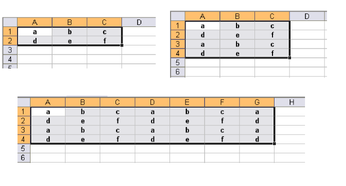
Figure 2: The result of filling an initial range twice: first by filling two additional rows, and then four columns.

Assumption 1.

We consider the spreadsheet grid to be infinite. Therefore, the user can start with a small spreadsheet and fill any desired number $r$ of rows and $c$ of columns with copies of the initial formulas. We assume also that there is no limit on the numbers used in the spreadsheet, so that we can represent the location of every cell in the spreadsheet by a number.

Definition 2.

The computing part of a spreadsheet $S$ is the fragment of it, used for filling the grid with formulas, in order to process the input data of variable size. The input part of this spreadsheet are those cells, which are not subject to filling and do not contain formulas referring to the cells filled. The output part of a spreadsheet is the last created row/column of cells.

We always assume that these three parts are indicated in the spreadsheets we discuss below, although spreadsheets used in everyday practice do not make this distinction clear.

Definition 3.

Computation of a spreadsheet is the act of marking the computing part of this spreadsheet and filling a certain number of rows and columns (in either order) by formulas from this part, to which the spreadsheet system (Excel in this paper) responds by evaluating the so created formulas. In particular, this process produces the output, which consists of the values computed in the output part.

Under Assumption 1 and Definitions 2 and 3 we can consider a spreadsheet as a program, with clearly identified areas for input, executable part and output. The process of filling allows one to use this program for processing input data of variable size. This is a crucial step, which allows us to describe the computing power of spreadsheets using common complexity classes.

Now we are going to define two crucial structural characteristics of spreadsheets. It will turn out that they determine their ability to express computations of certain complexity. Both characteristics are preserved by filling.

Definition 4.

A spreadsheet $S$ is row-organized, if all ranges to which formulas of $S$ refer are horizontal ones, i.e. rows.

Dually, $S$ is column-organized, if all ranges to which formulas of $S$ refer are vertical ones, i.e. columns.

Finally, $S$ is un-organized if it neither row-organized nor column-organized.

In all cases, references to the input part of $S$ are exempt from those limitations.

Definition 5.

A spreadsheet $S$ is row-directed if every formula refers only to cells and ranges located in rows above that one in which the formula is located.

Dually, $S$ is column-directed, if every formula refers only to cells and ranges located in columns located to the left of that one in which that formula is located.

$S$ is un-directed if it is neither row- nor column-directed.

Finally, $S$ is bi-directed if it is both row- and column-directed.

Again, references to the input part of $S$ are exempt from those limitations.

3 PRAM model

A PRAM machine $A$ consists of the following components:

1. Unbounded number of cells of global read-and-write shared memory, each one equipped with:

   1. Its own serial number, unique, counted from 1 on.

   2. Capacity to store one integer, initially set to 0.

2. Unbounded number of cells of global read-only input memory, each one equipped with:

   1. Its own serial number, unique, counted from 1 on.

   2. Capacity to store one integer, initially set to 0.

3. Unbounded number of processors, each one equipped with:

   1. Its own serial number $s,$ unique, counted from 1 on, and a constant $N,$ equal to the total number $p$ of active processors and a constant $M$ equal to the number of active cells of shared memory.

   2. Three private registers $i,j,k$ for storing integers, initially set to 0.

   3. Its own instruction counter, initially set to 1.

4. Program $\pi$, which is a list of consecutively numbered instructions of the following forms, and where $x$ is ranging over $i,j,k$ and $u,v$ are ranging over $i,j,k,s,N,M,M[i],M[j],M[k],M[s],I[i],I[j],I[k],I[s]$ and integer constants and $\ell$ ranges over integer constants:

   1. $x:=u$

   2. $x:=u\circ v$, where $\circ$ is among $\{+,-,*,/\}$

   3. $M[x]:=u$

   4. $M[x]:=u\circ v$, where $\circ$ is among $\{+,-,*,/\}$

   5. if $u<v$ then goto $\ell$

The number of private registers can be chosen arbitrarily. We needed some fixed limit, so we have decided to use 3 of them.

$M[x]$ stands for the shared memory cell whose address is $x,$ and $I[x]$ stands for the input memory cell whose address is $x.$

The input sequence $v$ of integers is located in the input memory cells, and $I[1]$ contains the length of the input sequence, including itself (so that the empty input sequence is passed to the machine as 1 in $I[1]$).

Then a fixed number of its processors (say $p$) is initialized, and a fixed number of shared memory cells (say $m$) is initialized. Typically $p$ and $m$ are adjusted to the length of $v.$

During the computation each of the processors follows this program. The state of $A$ at each time $t$ of its computation on input $v$ is defined to be the sequence of $p$ 4-tuples of integers and a sequence of $m$ integers: the $n$-th tuple is the state of the $n$-th processor, consisting of: the values of its local variables $i,j$ and $k,$ the value of its instruction counter, while the sequence of integers represents the content of the shared memory.

Initially (i.e., at time $t=0$) the values of local registers are 0, and the instruction counter 1, and the shared memory values are 0.

A single step of computation of $A$ corresponds to a parallel, simultaneous change of all $p$ 4-tuples and $m$ integers describing the processors and shared memory of $A.$

The effect of a reference to the local registers, in order to read or write, should be clear, if we say that $/$ is the integer division. References to the shared memory and input memory cells are more complicated. First of all, an attempt to read from a nonexistent input or shared memory cell (i.e., of address higher than $I[1]$ or than $p$, resp.) or to read from cells of numbers smaller than 1 is an error and the result of this operation is unpredictable: it may cause the machine to break and stop operating, or to retrieve some accidental value and continue computation.

An attempt to write to a shared memory cell of zero or negative number is permitted, but has no effect, and similarly if that number is higher than $p$. If more than one processor attempts to read from the same shared or input memory cell, all of them succeed and get the same value. If more than one processor attempts to write to the same shared memory cell, all the requests are executed, and the new value of that memory cell is the one written by the processor with the lowest serial number; the values written by the remaining processors get lost. Reading is performed before writing, so the processors which read from a shared memory cell to which other processors wish to write, get the “old” value. The model of PRAM with this policy of resolving read and write conflicts is called priority write Concurrent Read Concurrent Write PRAM, abbreviated CRCW PRAM.

Of course, the instruction counter is increased by one in such cases. The conditional instruction if $u<v$ then goto $\ell$ causes the instruction counter of a processor to be updated depending on the comparison of the values of $u$ and $v$ : if $u$ is less than $v$ then it is updated to $\ell$, otherwise it is incremented by 1. We always assume that $\ell$ is a positive integer not exceeding the total number of lines in $\pi$– note that the value of $\ell$ is hard-coded into the program. If the value of the instruction counter becomes higher than the number of lines in the program, the processors halts.

Thus, given a PRAM $A$ as above and its input vector $v$, the computation of $M$ on $v$ is represented by a finite or infinite sequence of states of $A$, which may but need not be constant from some moment on.

The result of computation of $A$ after $n$ steps is the content of the shared memory after completing that step.

Another, substantially weaker model of PRAM is EREW, short for Exclusive Read Exclusive Write, which results from CRCW by forbidding concurrent reads and writes altogether. Its advantage is that it is closer to real-life parallel computers than CRCW.

The programming language of our PRAM machines is extremely simple, but, as it is well-known, equivalent in computing power to even very rich ones, so indeed each processor separately has a universal computing power, equivalent to that of a Turing machine.

PRAM is a machine which can easily implement referential data structures, such as lists, trees, etc., as well as arrays. Therefore we use them without any further explanation.

4 Complexity theory

$p$ is the class of all functions computable by PRAMs with one processor and unbounded amount of memory, in time polynomial in the length of the input. In fact, the number of memory cells ever used in a computation cannot exceed the number of computation steps made.

In this paper we use the $P$-complete problem Circuit Value Problem (abbreviated CVP).

An instance of CVP is a sequence of $n$ Boolean substitutions (the reason for starting numbering from 2 is purely technical and explained below):

$$p_{2}:=conn_{2}(inputs_{2})$$

$$p_{3}:=conn_{3}(inputs_{3})$$

$$\ldots$$

$$p_{n}:=conn_{n}(inputs_{n})$$

The connectives $conn_{i}$ can be and, or and not. The first two of them have always two inputs, not has one input. Each of the inputs in $inputs_{k}$ can be either $true$, or $false$, or a variable $p_{i}$ with $i<k,$ indicating that the value of that variable should be used. For example, the following is a valid instance of CVP of size $n=4$ :

$$p_{2} :=and(true,false)$$

$$p_{3} :=or(true,p_{2})$$

$$p_{4} :=or(false,p_{3})$$

$$p_{5} :=not(p_{4})$$

One can then calculate the values of all variables in that instance, proceeding top-down: $p_{2}$ is $false$, $p_{3}$ is $true$, $p_{4}$ is $true$ and $p_{5}$ is $false.$

The CVP problem is that, given an instance of CVP, to decide if the last variable is $true$. That problem is known to be $P$-complete.

We encode CVP in various spreadsheets in order to demonstrate that they are unlikely to be efficiently parallelizable. For convenience, when we do so we use 0 in place of $false$, 1 in place of $true$, for variables we use their numbers as names (we have started numbering from 2, so this does not lead to confusing truth values with variables), and we drop all conventional symbols like $:=$, parentheses and commas, so that the above example is encoded by the spreadsheet shown in Figure 3.

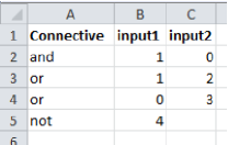
Figure 3: CVP instance in a spreadsheet.

$NC$ is the class of functions computable by PRAMs with polynomially many processors, using polynomially many shared memory cells and in time bounded by $\log^{k}n$ for some constant $k$, for input data of size $n$.

We often use the “big Oh” notation for the asymptotic growth of functions. In this notation, $P$ is the class of functions computable by a sequential (i.e., single-processor) program in time $n^{O(1)}$, while $NC$ is the class of functions computable in time $\log^{O(1)}n$ on a parallel computer using $n^{{O(1)}}$ processors.

It is a well-known fact that $NC\subseteq P,$ and it is widely believed, but remains unproven, that indeed $NC\neq P.$

This hypothesis is often rephrased as a statement, that there are problems decidable in polynomial time, which are inherently sequential, i.e., cannot be solved very fast by parallel machines. $NC$ is understood in this statement as “the” class of problems which can be solved fast in parallel.

If $NC\neq P$, then in particular $P$-complete problems cannot be solved by PRAMs in time $\log^{O(1)}n$.

Therefore CVP cannot be solved on a PRAM with polynomially many processors and polynomially many cells of shared memory in time $O(\log^{O(1)}n)$, where $n$ is the size of input and $k$ is a constant, unless $P=NC.$

In this paper we do not derive hypothetical lower bounds on the complexity of evaluating various classes of spreadsheets. Instead, we estimate the size of CVP instances, which are computable in the spreadsheets in question. Each time it is easy to translate the size of CVP instances we produce into the potential lower bounds.

5 Un-directed spreadsheets I: Complexity

It is obvious, that if the cells of a small initial spreadsheet $S$ are filled to create $c$ columns and $r$ rows of formulas, then the resulting spreadsheet can be computed in time polynomial in $cr$, given the initial $S$, the dimensions $c$,$r$ and the input data of $S$. More precisely, spreadsheet operators typically can be implemented by algorithms of time complexity linear in the size of their input ranges, with a few exceptions like FREQUENCY, which require complexity of order $O(n\log n)$. The largest possible range in a spreadsheet with $cr$ cells does not exceed $cr$ cells, so computing cells can be done in time $c^{2}r^{2}\log cr$. Determining the evaluation order requires topological sorting, which can be done in time linear in the number of inter-cell references, which does not exceed $c^{2}r^{2}$. Therefore in total we get the maximal possible computation time $O(c^{2}r^{2}\log cr)$.

In case of row-organized spreadsheets or column-organized spreadsheets we get the orders of $cr^{2}\log cr$ and $c^{2}r\log cr$, respectively, due to restricted sizes of ranges.

The following theorem is neither surprising nor difficult to demonstrate. It states in particular, that CVP is computable by spreadsheets.

Theorem 6.

There exists an un-directed, un-organized spreadsheet $S_{4}$, such that when it is extended to dimensions of either $n$ rows and $6$ columns or $6$ rows and $n$ columns, it computes the solution to the CVP problem of size $n$, given its description as input.

Proof.

A fully commented spreadsheet is provided as electronic appendix S4. ∎

The same behavior is demonstrated by a slightly more complicated spreadsheet $S_{5}$, which extended to yield $4r$ rows and $2c$ columns, computes the answer to a CVP instance of size $cr.$ So its full area is devoted to solving the instance of CVP. This spreadsheet is provided as electronic appendix S5.

The difference between $S_{4}$ and $S_{5}$ is that the former consists of two functionally separate fragments, which can be independently converted into row-oriented and column-oriented structure, as it is demonstrated in electronic appendix S4. In $S_{5}$ it is impossible, because it uses two-dimensional ranges in a crucial way.

6 Directed spreadsheets I: Algorithm for a restricted function set

At first, we restrict spreadsheets significantly, in order to formulate and prove our results in a simplified scenario.

First, we restrict spreadsheets to use only integer numbers.

Next, we restrict spreadsheets to just a few functions, here given in Excel syntax.

All of them are also found (perhaps in a slightly different syntactical form) in the competing spreadsheet systems, which therefore are also covered by the theorems we shall prove below.

6.1 Functions in restricted spreadsheets

6.1.1 Arithmetical functions

We use standard arithmetical functions: $+$, $\cdot$, $-$ and $/$.

6.1.2 Comparison functions

value1=value2

value1<value2

value1>value2

value1<=value2

value1>=value2

value1<>value2

value1 and value2 can be numbers, formulas or cell references to numbers. The result is TRUE if the arguments are in the specified relation, and FALSE otherwise.

6.1.3 Logical functions

IF(test,value1,value2)

If test is, refers or evaluates to TRUE, the function returns value1, if test is, refers or evaluates to FALSE it returns value2. In all other cases the result is a #VALUE! error.

IFERROR(value1,value2)

This function returns value2 if value1 is, refers to or evaluates to any error value, and value1 otherwise.

CHOOSE(index-num,value1,value2,…)

CHOOSE is a kind of generalization of IF, because in one formula it allows the choice among up to 29 possible values to be returned. index-num specifies which value argument is selected. index-num must be a number between 1 and 29, or a formula or reference to a cell containing a number between 1 and 29.

If index-num is $i$, CHOOSE returns value$i$.

AND(value1,value2,…) and OR(value1,value2,…)

compute the logical conjunction and disjunction of their arguments, respectively.

6.1.4 Address functions

We use two address functions: ROW() and COLUMN(), which return the number of row (column, resp.) od the cell in which they are located. In case they are given an argument, a reference to a single cell, they return the row (column, resp.) in which that reference is located.

6.1.5 Aggregating functions

MATCH(lookup-value,lookup-array,match-type)

lookup-value is the value to be found in a range specified by lookup-array. lookup-value can be a number, a formula or a cell reference to a number.

match-type in the spreadsheets we create is typically 0. It specifies how the spreadsheet matches lookup-value with values in lookup-array: MATCH finds the first value that is exactly equal to lookup-value and returns its relative position in the lookup-array.

If match-type is 1, then values in lookup-array are assumed to be sorted into an increasing order, and MATCH finds the first value that is larger or equal to lookup-value and returns its relative position in the lookup-array. If match-type is -1, then values in lookup-array are assumed to be sorted into a decreasing order, and MATCH finds the first value that is smaller or equal to lookup-value and returns its relative position in the lookup-array.

In all three cases, if no value is found which satisfies the criteria, the result is an error #N/A!. In case of match-type equal $\pm 1$ lookup-value is larger (smaller, resp.) than all values in the sorted lookup-array, the result is the number of the last non-empty cell in lookup-array.

INDEX(array,row-num,col-num)

array is a range of cells, row-num and col-num can be numbers, formulas yielding numbers or cell references to numbers. The result of the function is a value whose relative position in array is given by row-num and col-num. We use this full syntax exactly twice, otherwise array is a single column or row and one of the arguments is missing – its default value is 1.

6.2 Simulating spreadsheets by PRAMs

In this section, we are going to formulate and prove a theorem about evaluating spreadsheets by PRAM machines. In our model spreadsheets can be of unbounded size, so we can use asymptotic notation to describe the resources needed by a PRAM to execute a spreadsheet of a given size. The theorem below is formulated for row-organized row-directed spreadsheets, but of course its dual form for column-organized column-directed spreadsheets holds, too.

Theorem 7.

For any row-organized row-directed restricted spreadsheet $S$ there exists a program $\pi$ for EREW PRAM, such that if that spreadsheet filled to make $c$ columns and $r$ rows, the values of all its cells can be computed by $\pi$ run for $O(r\log cr)$ time on $c$ processors and $cr$ cells of memory, given the initial $S$, $c$, $r$ and the input data of $S$.

If $S$ is additionally row-organized, then the values of its cells in the last row can be computed by $\pi$ run for $O(r\log c)$ steps on a PRAM with $c$ processors and $c$ cells of memory.

Proof.

For each column of the spreadsheet we designate one processor, which will be responsible for it. Let the number of that processor will be equal to the number of the column.

Assume that first from the initial constant size range of $S$, rows are extended to the right to create $c$ columns, one by one starting from the top row. Then a number of so created rows is filled downwards to create $r$ rows.

The idea is to organize the computation of PRAM simulating the above procedure in rounds, where each round corresponds to creating one new row.

In order to evaluate formulas creating the row, PRAM must know what to evaluate. The codes for evaluating particular formulas are hard-coded into the program $\pi$ it executes. Observe that the initial $S$ has a constant number of rows and formulas, and they repeat in a circular fashion in the large spreadsheet created by filling. Hence the program is divided into a constant number of branches, one for each type of a column, which are executed by the processors responsible for such columns. The portion of code for each type of column is composed of a main loop, the body of which determines how to evaluate the constant number of formulas repeating in the column. Evaluating of formulas sometimes requires coordinated actions of all processors. The code to be evaluated in such cases is also provided in the body of the main loop.

For each round we assume that certain auxiliary data structures are available, which enable execution of the round sufficiently fast by PRAM. During each round, first the new values are computed, and then these structures are updated, so that they include the cells in the newly created row, as well.

Separately, we must explain how the auxiliary data structures are initialized before the first round, when they should contain information about input data.

6.2.1 Auxiliary data structures

We assume that during each round all the previously created columns and rows are stored in two copies. Each row is stored in two copies:

1. in the original form,

2. as a sorted array, where we sort and store two-element records consisting of the value from the original row and its original address.

Each column is stored in two copies:

1. in the original form,

2. as a balanced binary search tree (say: red-black tree), in which we store two-element records consisting of the value from the original row and its original address.

6.2.2 Initialization of auxiliary data structures.

Initially there is a constant number of rows and/or columns without formulas, containing input data. It is easy to see that we can relocate columns of input data into rows.

In order to create their sorted forms, we perform a logarithmic time parallel sorting algorithm using $c$ processors and linear amount of additional memory, like the one described in [5][Section 5.2]. This initialization takes $O(\log c)$ time.

Initial columns are of constant height, so the red-black tree of each of them is created by one processor, responsible for that column, in constant time.

6.2.3 Execution of a round. Computing formulas

Henceforth, PRAM must first evaluate formulas. The formulas to be computed refer only to data above themselves, so all of them can be evaluated independently in parallel. For each of the cells, it is done by a single processor, responsible for the column of that cell. The values of all functions except MATCH and INDEX can be obviously evaluated in constant number of steps. Note that COLUMN function can be evaluated, because each processor knows its serial number, equal to the column number. ROW on the other hand is evaluated by keeping a constant record of the advancing computation time.

If MATCH looks up a row, a sorted version of that row is in the auxiliary data structures, in which the processor can find the suitable value (and its accompanying address, which ought to be returned) using binary search in time $O(\log c).$

If MATCH looks up a column, a red-black tree version of that column is in the auxiliary data structures, in which the processor can find the suitable value (and its accompanying address, which should be returned) in time $O(\log r).$

In total, computing the new values takes $O(\log c+\log r)=O(\log cr)$ time.

6.2.4 Execution of a round. Updating auxiliary data structures.

The sorted copy of the newly created row is computed in $O(\log c)$ time using logarithmic time linear memory sorting employing all $c$ processors. Then all processors in parallel insert the new values from their columns into the corresponding red-black trees, in time $O(\log r)$.

In total, updating the necessary data structures takes $O(\log cr)$ time.

6.2.5 Cost of the algorithm

First, initialization of auxiliary data structures takes $O(\log cr)$ time. Then the simulation of the PRAM computation performs $r$ rounds, each of them takes $O(\log cr)$ time, so the total time is $O(r\log cr).$

The memory used is constant times $cr$.

For the second claim, in a row-organized spreadsheet there is no need to access columns, so we do not need to maintain red-black trees. Thus in this modified version each round can be completed in $O(\log c)$ time and the total running time is $O(r\log c).$

Moreover, if initially $S$ had $k$ rows, then every formula copied from $S$ either accesses one of the initial $k$ rows, or row at most $k$ levels above itself. Consequently we need to store at most $2k$ rows simultaneously, and therefore the total amount of necessary memory is $O(c).$ ∎

7 Directed spreadsheets II: Algorithm for a rich function set

The most significant differences between real-life spreadsheets and the simplified ones, which we have discussed so far, are:

1. More data types than just integers, most notably floating point numbers and text strings.

2. More functions are permitted.

7.1 More functions

Generally, functions provided in spreadsheet systems can be divided into two types basic types: scalar ones, which have only several single cell arguments (including functions without any arguments), and aggregating ones, which have at least one argument, which is a range. There are functions which can be used both as scalar and aggregating ones. Therefore we apply this distinction to formulas in spreadsheets, where each function occurrence in a formula is, depending on the particular syntax used in it, either scalar or aggregating.

7.1.1 Scalar functions

Scalar functions can be easily incorporated into our discussion. If a scalar function is added simultaneously to the syntax of PRAM programs and to the spreadsheets, the two systems remain in the same relation as indicated in our theorems. The proofs can easily be adapted.

7.1.2 Aggregating functions

In order to avoid considering hundreds of functions found in real life spreadsheets, the approach we take here is to consider array formulas, which can equivalently express great majority of aggregating functions present in spreadsheets, and many functions which cannot be expressed by other means. After introducing them, we formulate a general condition on array formulas, which guarantees that spreadsheets which use them can be evaluated by a PRAM within the same time bounds as MATCH and INDEX functions, the only aggregating functions we permitted so far. In particular, this means that Theorem 2 remains true for spreadsheets which contain array formulas which meet this condition.

The array formulas we use in this paper are constructed as follows:

First the inner expression is formed from scalar functions, but whose arguments are rows or columns (of identical sizes) instead of single cells. Single cells or constants appearing in the formula are interpreted as rows or columns of identical values. Then the result of this expression is again a row or column, resulting by computing the functions at each position independently. In particular, an array formula cannot contain rows and columns simultaneously.

Finally, the inner expression is an argument of an aggregating function, which takes an arbitrary number of elements and returns a single number, such as, e.g., SUM, MAX or AVG. This function is applied to the row or column of results of the expression and yields a single number, which is the value of the array formula.

Array formulas are entered by pressing Ctrl+Shift+RETURN and are marked by a pair of braces {} around, which are introduced by the system (and not typed in by the user). This identifies them for the spreadsheet system and invokes their special evaluation algorithm.

Example 8.

Let us consider the following the formula and its context shown in Figure 4.

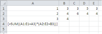
Figure 4: Array formula and its context

The outer aggregating function is SUM, and its inner expression is (A1:E1=A3)*(A2:E2=B3). In this situation A3 and B3 are treated as rows of five 3s and five 4s, respectively. This way equality can be used to compare a range and a single cell, and returns, for position in the rows, TRUE if its arguments are equal and FALSE otherwise. For multiplication, TRUE is treated as 1 and FALSE as 0. Carrying out these calculations at each position independently, we get a row of values 0, 1, 0, 0, 1. Now SUM applied to it yields 2 and this is the result of the array formula. Thus the final result is the count of positions, at which rows 1 and 2 contain the pair $(3,4)$ (i.e., the same as in cells A3 and B3). Consequently, we get the same function as computed by COUNTIFS(A1:E1,A3,A2:E2,B3), aggregating function present in the newest editions of Excel.

Example 9.

Another example consists of five formulas is shown in Figure 5.

Figure 5: Five array formulas and their context

The formulas compute the variance of the subset of those numbers in row 2, which are accompanied in row 1 by a value identical to A3. Indeed, the first formula (located in A4) computes the sum of those values, the next formula (located in A5) calculates the number of those values, the one in A6 calculates the mean, and finally the next two, found in A7 and A8, calculate the variance according to the formula ${\mathbb{V}}(X)={\mathbb{E}}((X-{\mathbb{E}}(X))^{2}).$

The actual numerical result is not so important. The formula in A6 computes the equivalent of the AVERGAGEIFS function found in the newest versions of Excel, while A8 computes the equivalent of the DEVPIFS function, that hypothetically would compute the variance of the whole population of elements satisfying multiple criteria - however, this function is not present in Excel.

We have given an example of a spreadsheet function, which can be equivalently expressed as an array formula, and example of an array formula whose functionality cannot be expressed by a single standard spreadsheet function.

Theorem 10.

For any row-organized row-directed spreadsheet $S$ which, in addition to functions permitted in restricted spreadsheets, uses array formulas which

1. have SUM as the outer aggregating function,

2. whose inner expressions use only multiplication, addition, subtraction and comparison operators=, <=, <, >=, >, <>, applied directly to compare argument ranges and cells,

3. moreover, have at most one comparison operator other than = applied to compare a range to a single cell,

there exists a program $\pi$ for EREW PRAM, such that if that spreadsheet filled to make $c$ columns and $r$ rows, the values of all its cells can be computed by $\pi$ run for $O(r\log cr)$ time on $c$ processors and $cr$ cells of memory, given the initial $S$, $c$, $r$ and the input data of $S$.

If $S$ is additionally row-organized, then the values of its cells in the last row can be computed by $\pi$ run for $O(r\log c)$ time on $c$ processors and $c$ cells of memory.

Proof.

It suffices to demonstrate how the evaluation of an array formula of the above described form can be incorporated into the algorithm described in the proof of Theorem 2.

The inner expression is built from ranges, cells and comparisons using multiplication, addition and subtraction. In particular, the inner expression can be thus equivalently expressed as a sum of products of ranges, cells and comparisons. Since the outer aggregating function is SUM, it suffices to explain how to evaluate an array formula whose inner expression is a single product of ranges, cells and comparisons. Single cells as factors in the product can be moved outside of the outer SUM, hence finally we have an array formula of the form: outer aggregating function SUM and inner expression is a product of expressions of the following types:

1. ranges U,

2. comparisons between ranges U$r$W, where $r$ is any of =, <=, >=, <, >, <>,

3. equality comparisons between ranges and single cells V=C,

4. at most one inequality comparison between a range and a single cell X$r$D, where $r$ is any of <=, >=, <, >.

7.1.3 Auxiliary data structures

If the ranges in the array formula are rows, the auxiliary data structure is prepared as follows: for every subset of already existing rows, which potentially may play together the roles of U and W ranges above, the values found in the ranges and the results of comparisons U$r$W are multiplied in each column separately. Then the records formed from the resulting values together with the values found in the rows which play the role of ranges V are sorted according to the values in the V rows and the X row. Which of the rows V are more or less significant in the sorting is unimportant, but the single X row (if present) is the least significant one in the sorting.

Finally, for the so created array prefix sums of results of multiplications are computed and stored as an array (i.e., the first value in the prefix sums array is the first value from the original sorted array, the second value in the prefix sums array is the sum of the first and second value from the original sorted array, the third value in the prefix sums array is the sum of the first, second and third value from the original sorted array, and so on).

If the ranges in the array formula are columns, the auxiliary data structure is prepared as follows: for every subset of already existing columns, which potentially may play together the roles of U and W ranges above, the values found in the ranges and the results of comparisons U$r$W are multiplied in each row separately. Then the records formed from the resulting values together with the values found in the columns which play the role of ranges V are stored in an red-black tree according to the values in the V rows and the X row. Again the single X row (if present) is the least significant one in the sorting. Apart from that, in the red-black tree each node stores additionally the sum of all results of multiplications in the subtree rooted at this node.

7.1.4 Initialization of auxiliary data structures.

Initially there are only constantly many rows without formulas, consisting of input data.

In order to create their sorted forms, we perform a logarithmic time parallel sorting algorithm using $c$ processors and linear additional memory. Then prefix sums are computed according to the algorithm described in [3][Section 30.1.2]. In total, the initialization takes $O(\log c)$ time.

Initial columns are of constant height, so the red-black tree of each of them is created by one processor, responsible for that column, in constant time. Computing sums of values from column X is also immediate. This initialization takes constant time.

7.1.5 Execution of a round. Computing formulas

PRAM must first evaluate array formulas in the newly created row. The formulas to be computed refer only to data above themselves, so all of them can be evaluated independently in parallel. For each of the cells, it is done by a single processor, responsible for the column of that cell.

In case of row ranges, when the values of single cells C are already known, binary search is performed on the ordered array to find the first and the last element whose V values agree with the C values. Between them there are records with identical values in V rows, ordered by their values in row X. Using further binary search, we find the point indicated by the value from cell D. The values in the interval between this point and one of the previously identified elements should be summed up. In order to do so, we use the array with prefix sums. The required sum is the difference between prefix sum corresponding the rightmost of them minus prefix sum corresponding to the leftmost of them. This procedure takes $O(\log c)$ time.

In case of column ranges, when the values of single cells C are already known, the procedure is similar to the one used for rows. The key observation is that if the processor searches for an element in the tree, it can sum the sums recorded in the left sons of nodes at which it descends towards the right son. When the required element is found, the sum of those sums is precisely the prefix sum corresponding to that element. With this remark, the previously used computation can be easily simulated, and takes $O(\log r)$ time.

In total, computing the new values takes $O(\log c+\log r)=O(\log cr)$ time.

7.1.6 Execution of a round. Updating auxiliary data structures.

The sorting of the auxiliary rows and creating the array with prefix sums are performed in $O(\log c)$ time using the algorithms we have used in initialization, using all $c$ processors.

Updating red-black trees by inserting the new values from their columns and updating the sums is done in $O(\log r)$ time.

In total, updating the necessary data structures takes $O(\log cr)$ time.

7.1.7 Cost of the algorithm

First, initialization of auxiliary data structures takes $O(\log cr)$ time. Then PRAM performs $r$ rounds, each of them takes $O(\log cr)$ time, so the total time is $O(r\log cr).$

The memory used is constant times $cr$. ∎

Generally, the following standard, important functions found in spreadsheet systems can be equivalently expressed by (one or a few) array formulas which obey the criteria of Theorem 7: SUM, SUMIF, COUNT, COUNTIF, AVG, AVGIF, STDEV, SUMX2PY2, SUMX2MY2, SUMPRODUCT.

Two more functions, introduced for the first time in Excel 2007: SUMIFS and COUNTIFS are covered in a limited form: if at most one of the criteria in the function is an inequality, then it can be expressed by an array formula satisfying the assumptions of Theorem 10.

7.2 Floating point numbers and strings

Floating point numbers can be added to the PRAM model by allowing the register and memory cells to store them. All theorems formulated for relations between classical PRAMs and spreadsheets with integers hold analogously when formulated for PRAMs and spreadsheets with floating point numbers, and the proofs remain the same.

Text strings do not pose any significant problem. Indeed, there is no aggregating function for strings in Excel. Hence, the only functions which use them are scalar ones, and they can be added very much the same way as scalar functions for integers.

8 Directed spreadsheets III: What can they compute?

At this point, we have demonstrated that directed spreadsheets can be evaluated by quite efficient parallel algorithms.

Two questions arise naturally:

Is the estimate from the previous section optimal, or is there a chance for further improvement?

What is the set of functions, which can be implemented in directed oriented spreadsheets?

In order to answer both questions simultaneously, we are going to demonstrate now that there exists a spreadsheet program, with the following property: any given CRCW PRAM $A$ can be encoded in a can be simulated by a row-organized row-oriented spreadsheet.

Theorem 11.

There exists a row-organized row-directed spreadsheet using restricted function set, which is able to simulate any PRAM $A$ for which $p=m$, so that columns rows correspond to processors of $A$ and rows correspond to computation time.

Precisely speaking, there exists a single spreadsheet $S_{1}$ consisting of 19 cells (A2 to A20) with formulas, one row for input and a separate input area for input interpreted as a program, such that for every CRCW PRAM $A$ with program $\pi$, $p$ processors and $p$ cells of shared memory, and for every input vector $v$ for $A$, if one

1. pastes the encoding of $\pi$ into the program area of $S_{1}$

2. marks and fills the initial range A2:A20 to the right creating $p$ columns (corresponding to the processors and shared memory cells of $A$)

3. selects the rows from 11 to 20 of these $p$ columns and fills downward so that the bottom row of the new range is $10t+10$,

4. pastes into $S_{1}$ the input vector $v$ of $A$ in the first row,

then the cells of the bottom 10 rows compute the state of $A$ after $t$ steps of computation on $v$.

This means, that the spreadsheet created from $S_{1}$ in steps 1, 2 and 3 performs the first $t$ steps of the computation of $A$ on every input, i.e., it is a simulator of $A.$

Proof.

Electronic appendix S1 is the implementation of PRAM in a spreadsheet with explanation of the formulas used for that purpose.

Below we highlight the main issues of the construction of $S_{1}$.

Because $p=m$ in $A$, we may assign a processor to each shared memory cell and make it responsible for its operation. So in every step of computation it will perform its own action, and then take care of the actions of the memory cell.

Conceptually, the main difficulty in the construction which is presented below is that PRAM is a “read and write” machine, i.e., every processor can both read data from and write data to any shared memory cell, while spreadsheet is a computation model in which cells (which can be thought of as simple processors) can read data only from other locations, and are allowed to write only to the shared memory cell they are associated with, and moreover only once. This means that in the course of simulation we will have to simulate writing by other means. The idea is that any processor willing to write its contents to some shared memory cell, has to announce this. Then all processors use function MATCH to search for the announces of writes to their shared memory cells, and if there is one, fetch using INDEX the leftmost one, according to the priority write CRCW conflict resolution policy.

Because processors located in spreadsheet cells are executed only once, it is necessary to simulate a PRAM by a spreadsheet which has a separate cell for every processor at every time instant, so the number of necessary cells is linear in the number of processors of the PRAM multiplied by the running time of the PRAM. ∎

At the time of this writing, Excel 2013 (TM) allows the maximal size of a single worksheet to be 1,048,576 rows by 16,384 columns, hence, according to our construction, S1 can (theoretically) simulate a PRAM with about 16 thousands processors and cells of shared memory, and running for slightly more than 100 thousands parallel steps. In practice it would be extremely slow if used for simulating PRAM computations of the maximal size, and might require very large amounts of RAM to be installed on the computer to fit in memory. We also provide another simulator $S_{6}$, permitting structural programming with while-endwhile and if-endif rather than goto jump instructions. It is available as electronic appendix S6.

This construction provides answer for our questions:

1. There is not much room for improvement over Theorems 2 and 3. Indeed, they offer $O(r\log cr)$ and $O(r\log c)$ algorithms for PRAM with $c$ processors and $O(cr)$ and $O(c)$ cells of memory, depending on whether the spreadsheet is only row-directed or additionally also row-organized. On the other hand, every PRAM computation taking time $t$, using $c$ processors and $c$ cells of memory can be simulated in a spreadsheet with $c$ columns and about $10t$ rows.

2. The set of computations expressible in row-directed spreadsheets is indeed very rich, and it includes a natural parallel complexity class.

It is worth noting, that accordinng to the results already proven, we have the following.

Corollary 12.

Spreadsheets $S_{1}$ and $S_{6}$ are universal row-oriented row-organized spreadsheets.

Proof.

Given a row-oriented row-organized spreadsheet $S$, one can derive an EREW PRAM program $\pi$, computing the same function as $S$. This $\pi$ can be encoded and provided as (a part of) input to either $S_{1}$ or $S_{6}$, which can execute it.

If the initial $S$ has $c$ columns and $r$ rows, then $\pi$ should be run on a PRAM with $O(c)$ processors and memory cells and $O(r\log c)$ time. Then, in order to simulate it, $S_{1}$ and $S_{6}$ need $O(c)$ columns and $O(r\log c)$ rows.

Thus the overhead of simulating a spreadsheet by the universal one is logarithmic, typical for other universal devices. ∎

The interest in the corollary is that $S_{1}$ and $S_{6}$ use only functions from the restricted function set of Section 6. Therefore this result indicates that the restricted function set forms a kind of core of the spreadsheet language of formulas, at least for the row-oriented row-organized ones.

Thus, in an attempt to create a theoretical model of spreadsheets, this restricted function set is a candidate to serve as the set of basic operations, from which the remaining one can be defined. It would be very much like the relational algebra and its role in the theoretical formalization of relational databases. However, one should remember that our proof concerns only row-oriented row-organized spreadsheets, created from a small initial spreadsheet by filling.

9 Directed spreadsheets: A parallel programming language

Because of the tight relationship between row-organized row-directed spreadsheets and PRAM computations, we postulate that spreadsheets can become a programming language for specifying scientific parallel computations on very large datasets. An important factor is that the computation time of the PRAM and its memory consumption are directly related to the dimensions of the spreadsheet, and thus can be reasonably well controlled by the programmer. Moreover, parallel evaluation algorithms for such spreadsheets are designed for EREW PRAM, closer to practical parallel computing facilities than CRCW PRAM.

From the end-user’s point of view, specifying massive parallel computations by designing spreadsheets does not require prior programming experience and is likely to be accessible for scientists and industry. It can be offered according to the increasingly popular “Software as Service” paradigm.

Below we describe how such system might work.

1. The user prepares a small initial spreadsheet application.

   1. The user designs the formulas.

   2. The user tests the formulas carefully on a small portion of data using Excel or some other existing spreadsheet software on a single machine, filling the spreadsheet with the prepared formulas.

   3. The user estimates the amount of data to be processed.

2. The user submits the spreadsheet and the complete set of data to the parallel computation facility, indicating:

   1. the location where the input data should be pasted into the spreadsheet

   2. the number of rows and columns for which the initial spreadsheet formulas should be filled.

3. The facility estimates the computation cost and asks the user for permission to execute it.

4. The user accepts the cost or aborts the procedure.

5. The facility executes the task.

6. The facility sends the computation results back to the user.

7. The facility asks the user if he/she is interested in extending the computation on the same dataset.

8. The user makes the decision.

9. If the user considers continuation of the computations, the facility sends him/her the rows necessary to continue the computation.

As one can observe, the above idea is a kind of non-interactive spreadsheet, very much like sed is a non-interactive text editor.

The same approach can be used to execute computations specified by means of row-directed but not necessarily row-organized spreadsheets. The fundamental drawback of this class is their much higher memory consumption during evaluation.

One should keep in mind, however, that the above idea requires considerable amount of further work to become available in practice. First of all, EREW PRAM algorithms we demonstrate in this paper must be suitably adapted to the architectures of existing parallel or distributed computation systems. Next, the language of spreadsheets should be enriched by suitable formula shorthands, making programming easier – the formulas used in our electronic appendix spreadsheets S1 and S6 are anything but simple and natural, even though they implement only bare-bones programming languages. An alternative might be a tool external to the spreadsheet, translating a richer language into the formulas composed from the basic functions. Anyway, in order to be successful, the resulting enriched language of formulas should be a reasonable compromise between the original language of spreadsheets, which has very strong data analysis component and no support for programming constructs, and the PRAM programming language, which has no data analysis primitives.

10 Bi-directed spreadsheets: Complexity

A bi-directed, column organized spreadsheet extended to dimensions $r$ and $c$ can be, according to Theorem 2, evaluated on a PRAM using $O(cr)$ processors and $O(cr)$ cells of memory and

1. in time $O(c\log r)$ if treated as column-organized column-directed.

2. in time $O(r\log cr)$ if treated as row-directed.

One might be tempted to believe that it is possible to combine somehow those two methods together to yield a parallel evaluation algorithm of even better time complexity. Optimally, it might seem plausible that time complexity $O((\log c\log r)^{{O(1)}})$ could be achieved.

However, we prove below that there is no evaluation algorithm of this complexity unless $P=NC,$ an unlikely event.

Theorem 13.

There exists a bi-directed, column-organized spreadsheet $S_{3}$, such that when it is extended to dimensions of $3n$ rows and $8n$ columns, it computes the solution to the CVP problem of size $n$, given its description as input.

Proof.

The main idea is to implement CVP “diagonally”, two fully commented implementations are provided in an electronic appendix S3. One of them is conceptually simpler, but uses two-dimensional INDEX calls. The other is even column-organized, but technical complication is the price to pay for this structural property. ∎

Bi-directed spreadsheets are clearly more restrictive than those which are directed in one dimension only. Author’s personal experience from the development of $S_{3}$ is that the bi-directed structure is quite unnatural, especially in the column-organized version. Otherwise very simple computation of CVP required a significant effort to be programmed. At the same time this structure does not seem to offer any noticeable advantage in terms of complexity of evaluation.

11 Un-directed spreadsheets II: What can they compute?

After a successful implementation of a PRAM in a row-directed spreadsheet and demonstrating that a large class of PRAM computations can be expressed in spreadsheets, it seems natural to attempt a similar goal for un-directed ones, too.

We demonstrate below, that one can create an un-directed row-organized spreadsheet which implements PRAM in a much more flexible way than the row-directed row-organized one.

Theorem 14.

There exists a restricted row-organized (but not row-directed) spreadsheet $S_{2}$ consisting of 21 cells (A2 to A22) with formulas using restricted set of functions, one row for input and a separate area for input interpreted as a program and for a value of $p$, such that for every CRCW PRAM $A$ with program $\pi$ for every input vector $v$, if one

1. pastes the encoding of $\pi$ into the program area of $S_{2}$

2. marks and fills the initial range A2:A22 to the right for $q$ columns,

3. selects rows 13:22 of these $q$ columns and fills downward so that the bottom row of the new range is $10t+12$,

4. pastes into $S_{2}$ the input vector $v$ of $A$ in the first row;

5. inserts a number into the input cell $p$

then the cells at the intersection of the bottom 10 rows with $p$ columns of numbers from $q-p-q(modp)$ to $q-q(modp)$ compute the state of $A$ after $t*(q/p-1)$ steps of computation on $v$.

Informally, the spreadsheet $S_{2}$ above is able to simulate any PRAM $A$, for which $p=m$ in such a way, that filled to $10t$ rows and $q\geq p$ columns, it can utilize this computation area to encode a PRAM with $p$ processors and $p$ cells of shared memory, running for $tq/p$ time. Moreover, the parameter $p$ is a part of the input, so only the whole input specifies, how many processors will be used in the computation. In particular, for $p=1$, this results in a fully sequential computation of length $tq.$

Proof.

The commented spreadsheet is provided as electronic appendix S2. However, it is recommended that the reader first analyses S1, on which S2 is based. ∎

It is instructive to compare $S_{5}$ from Section 5 with the present $S_{2}$. It seems at the first glance that the former is a special case of the latter. However, it is not the case. During the whole computation expressed in $S_{5}$ it is always possible to refer to the values computed in the past, no matter how distant. In $S_{2}$ the simulated PRAM can only refer to the values computed in the previous step of simulation. This indicates the difficulty of describing the computations of a spreadsheet by a machine model. In a spreadsheet, every cell is computed exactly once, but its value remains accessible forever. In typical machine models of computation, memory locations can be reused (overwritten), but once this is done, their old values become inaccessible.

12 Directed spreadsheets: Limitations

First of all, macros and user-defined functions written in general purpose programming languages, such as Visual Basic in Excel are excluded from the spreadsheets we analyze for the reason that in their presence all our above considerations become futile. Indeed, in their presence spreadsheet cells become mere output locations where the results of absolutely unrestricted computations of the macros and functions are written. Therefore the structure of the spreadsheet does not reveal any information about how its results are computed.

Our presentation does not cover all functions of spreadsheets. We would like to mention a few of them here, explaining the reason why they are excluded from our analysis.

OFFSET is a function which differs significantly from all other functions mentioned in this paper. It allows the user to specify an arbitrary range of cells, whose location is determined by the numerical arguments of OFFSET. INDEX in its full, two-dimensional syntax is similar in purpose and function. However, there is a fundamental difference between them. In the case of OFFSET calls their arguments are calculated at runtime and only then it becomes known, what cell each OFFSET call refers to. In particular, when this function is used, it is impossible to determine, before executing the spreadsheet, if circular references are created, if the spreadsheet is row-organized or row-directed. Generally, all features of spreadsheets which organize our discussion in this paper become meaningless in the presence of OFFSET. The full syntax of INDEX to the contrary, has a two-dimensional range as an argument limiting the area where the reference is created, and the full dimensions of this range is used to determine if circular references are created. This check is performed before running the spreadsheet.

Functions ADDRESS combined with INDIRECT can give a similar effect, since the former can be used to create a text address of any cell whose numerical coordinates are passed as arguments, and the latter transforms that text into the actual reference.

SUMIFS and COUNTIFS are allowed in Section 7 in a limited form. The complete form, which permits specifying two (or more rows) with inequality-type criteria and an additional row whose values should be added, refers to an unsolved problem in the theory of algorithms. If we consider the values in the first two rows as coordinates of points in the plane and the values in the third column as values located in those points, then specifying inequality-type criteria for summation or counting amounts to summing or counting the elements in an arbitrary quadrant of the plane. There is currently no data structure and algorithm known to allow for inserting points with values and summing values from any quadrant in time logarithmic in the number of specified points. However, there is no proof that this is impossible, either.

Circular references break the relation between the computation cost and the dimensions of the spreadsheet, because every cell is potentially recomputed many times. Moreover, the principle of direction becomes difficult to formulate. Electronic appendix S7 is the implementation of a PRAM in a spreadsheet with circular references. It is completely analogous to S1, except that it does not require creating additional rows. Instead, one has to enable circular references in the Excel options and change the value of the red SWITCH cell to 1 to run the computation. Inserting 0 in this cell resets the simulator to the initial state.

Presence of circular references brings about a completely new phenomenon in the spreadsheets – nondeterminism. Consider a three-cell example in Figure 6.

Figure 6: An example of nondeterminism in a spreadsheet with circular references. If the value of A1 is changed to 1, either A2 or B2 changes its value, but it is a nondeterministic choice, which one

If in this situation we change the value of A1 to 1, both A2 and B2 should be recomputed, because both depend on A1. Their contents are absolutely symmetrical. Which one will be recomputed first is decided by the spreadsheet cell recomputation mechanism. Recomputation changes its value from 0 to 1, and thereby prevents the other cell from changing the value from 0 to 1. Thus the spreadsheet breaks the symmetry between the contents of A2 and B2 and no logical examination of the formulas in the spreadsheet can determine which cell will change its value to 1 and which won’t. Therefore the characterization of the expressive power of spreadsheets with circular references most likely should refer to nondeterministic complexity classes.

13 Summary and related research

We have turned spreadsheets into a class of algorithms, by assuming that they are small templates, which are filled to a larger area of the grid to process data of variable size.

Under this scenario we have identified simple structural properties of spreadsheets, defined in the terms of the pattern of references between cells, which determine the complexity of the expressible computations.

One of the classes of spreadsheets appears to correspond closely to a natural parallel complexity class. It is therefore a reasonable candidate to become a general purpose parallel programming language dedicated for users without programming training.

There was very little previous research on the computational power of spreadsheets. The papers [1], [9] and [10] demonstrate simulations of various algorithms and models o computation using spreadsheets, but without any intent to estimate the full power of this computation paradigm. Paper [12] demonstrates how to implement relational algebra queries in spreadsheets (which turn out to be column-organized, but not necessarily column-oriented).

Electronic appendices

Electronic appendices can be downloaded from author’s Web page
http://www.mimuw.edu.pl/~jty/Spreadsheets.
Generally, spreadsheets referred to as S$i$ has name Tyszkiewicz_S$i$.xlsx there.

References

- [1] Mark Bernstein. Using spreadsheet languages to understand sequence analysis algorithms. Computer Applications in the Biosciences, 3:217–221, 1987.
- [2] Elissa J. Chesler, Sandra L. Rodriguez-Zas, Jeffrey S. Mogil, Ariel Darvasi, Jonathan Usuka, Andrew Grupe, Soren Germer, Dee Aud, John K. Belknap, Robert F. Klein, Mandeep K. Ahluwalia, Russell Higuchi, and Gary Peltz. In silico mapping of mouse quantitative trait loci. Science, 294(5551):2423, 2001. In Technical Comments.
- [3] Thomas T. Cormen, Charles E. Leiserson, and Ronald L. Rivest. Introduction to algorithms. MIT Press, Cambridge, MA, USA, first edition, 1990.
- [4] Mirosoft Corp. Excel on-line help system. http://office.microsoft.com/en-us/excel-help/.
- [5] Alan Gibbons and Wojciech Rytter. Efficient parallel algorithms. Cambridge University Press, 1988.
- [6] Andrew Grupe, Soren Germer, Jonathan Usuka, Dee Aud, John K. Belknap, Robert F. Klein, Mandeep K. Ahluwalia, Russell Higuchi, and Gary Peltz. In silico mapping of complex disease-related traits in mice. Science, 292(5523):1915–1918, 2001.
- [7] Thomas Herndon, Michael Ash, and Robert Pollin. Does high public debt consistently stifle economic growth? a critique of Reinhart and Rogoff. Technical report, Political Economy Research Institute, University of Massachusetts, 2013.
- [8] Report of JPMorgan Chase & Co. Management Task Force Regarding 2012 CIO Losses. Technical report, 2013.
- [9] I. M. Premachandra. Modeling a Turing machine on a spreadsheet: a learning tool. International journal of Information and Management Sciences, 4(2):81–92, 1993.
- [10] E. Rautama, E. Sutinen, and J. Tarhio. Excel as an algorithm animation environment. In ITiCSE ’97: Proceedings of the 2nd conference on Integrating Technology into Computer Science Education, pages 24–26, New York, NY, USA, 1997. ACM.
- [11] Carmen M Reinhart and Kenneth S Rogoff. Growth in a time of debt. Technical report, National Bureau of Economic Research, 2010.
- [12] Jerzy Tyszkiewicz. Spreadsheet as a relational database engine. In Proceedings of the 2010 International Conference on Management of Data, SIGMOD ’10, pages 195–206, New York, NY, USA, 2010. ACM.