Finite size scaling study of $N_{\text{f}}=4$ finite density QCD on the lattice

Abstract

We explore the phase space spanned by the temperature and the chemical potential for 4-flavor lattice QCD using the Wilson-clover quark action. In order to determine the order of the phase transition, we apply finite size scaling analyses to gluonic and quark observables including plaquette, Polyakov loop and quark number density, and examine their susceptibility, skewness, kurtosis and Challa-Landau-Binder cumulant. Simulations were carried out on lattices of a temporal size fixed at $N_{\text{t}}=4$ and spatial sizes chosen from $6^{3}$ up to $10^{3}$. Configurations were generated using the phase reweighting approach, while the value of the phase of the quark determinant were carefully monitored. The $\mu$-parameter reweighting technique is employed to precisely locate the point of the phase transition. Among various approximation schemes for calculating the ratio of quark determinants needed for $\mu$-reweighting, we found the Taylor expansion of the logarithm of the quark determinant to be the most reliable. Our finite-size analyses show that the transition is first order at $(\beta,\kappa,\mu/T)=(1.58,0.1385,0.584\pm 0.008)$ where $(m_{\pi}/m_{\rho},T/m_{\rho})=(0.822,0.154)$. It weakens considerably at $(\beta,\kappa,\mu/T)=(1.60,0.1371,0.821\pm 0.008)$ where $(m_{\pi}/m_{\rho},T/m_{\rho})=(0.839,0.150)$, and a crossover rather than a first order phase transition cannot be ruled out.

I Introduction

The 4-flavor QCD is a good testing ground for finite temperature and chemical potential analyses before studying the physically more relevant case of the 3-flavor theory. In fact, since the 4-flavor theory can be described with the staggered fermion formalism without rooting, new ideas to explore QCD with finite density have first been tried out in this theory Fodor and Katz (2002); D’Elia and Lombardo (2003); Kratochvila and de Forcrand (2006).

More fundamentally, the phase diagram of the 4-flavor theory is expected to have a structure well suited for exploratory studies at finite density. With massless quarks, as shown in Fig. 1(a), a continuous line of first order phase transitions connects the temperature and chemical potential axes. When the quark mass, $m_{q}$, is increased, the first order phase transition at zero density turns into a crossover beyond some value of $m_{q}$, while the transition at zero temperature and finite density remains first order as shown in Fig. 1(b). Consequently the first order line up to some value of the chemical potential also turns into a crossover. Hence a critical end point is expected at a finite chemical potential, which is reminiscent of the situation for the 3-flavor theory with the physical spectrum of up, down and strange quarks. It is empirically known Fukugita et al. (1990a); Iwasaki et al. (1996) in the zero density case that the first order phase transition persists up to a relatively large quark mass in the 4-flavor theory. Therefore one should be able to probe the region of the transition line with a reasonable computational cost, and learn much about the physical characteristics of the transition before tackling a more difficult 3-flavor theory.

A powerful method for resolving the nature of phase transition is the finite size scaling analysis. While this method has been extensively exploited in lattice QCD studies at finite temperatures, the situation appears quite different at non-zero baryon density. This is partly due to the fact that, in the phase-reweighting procedure for numerical simulations at non-zero density, the averaged phase-reweighting factor is expected to decrease exponentially as the lattice volume increases, leading to a loss of control of statistical averages of observables. In addition the calculation of the quark determinant necessary for evaluating the phase is computationally very expensive.

We note, however, that the former problem does not necessarily preclude finite-size scaling analyses as long as the reweighting factor stays reasonably away from zero over the range of lattice volumes needed for the analysis. This is a dynamical question, and as we have shown in Ref. Takeda et al. (2012a) the averaged phase-reweighting factor becomes larger for larger temporal lattice sizes. Concerning the latter, the reduction of the quark determinant Danzer and Gattringer (2008); Nagata and Nakamura (2010) and the recent development of computing technology including high speed GPGPU have significantly extended the range of lattice sizes for which the determinant is calculable in practice. In this article we therefore make a serious attempt at finite size scaling analyses for non-zero density QCD.

The Kentucky group Li et al. (2010) studied the phase structure of the 4-flavor theory using the canonical approach employing the Wilson-clover quark action. They observed an S-shaped structure in the chemical potential versus quark number plot, which they took to be an indication of a first order phase transition. The study was only on a single lattice volume of $6^{3}\times 4$ and with relatively low statistics, however, so this may not be taken as a conclusive statement. From the point of view of universality, it is important to check the phase structure by using different approaches. Accordingly, we also employed the Wilson-clover quark action, but adopted the grand canonical approach, and performed a finite size scaling study to learn how we can quantitatively resolve the order of the transition.

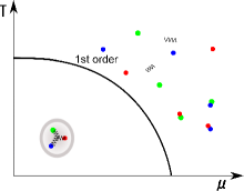
(a)

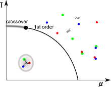
(b)

Figure 1: Phase diagram on the $(\mu,T)$ plane expected for 4-flavor QCD for (a) massless quarks, and (b) heavy quarks.

The rest of the paper is organized as follows. We briefly discuss the phase reweighting method and parameter reweighting for $\mu$ in Sec. II and III, respectively. Simulation parameters are summarized in Sec. IV. After defining the observables we measure in Sec. V, we present our finite size scaling analysis using susceptibility, skewness, kurtosis and the Challa-Landau-Binder cumulant for a variety of gluonic and quark observables in Sec. VI. By combining with results of zero density simulation, we describe a sketch of the global phase diagram in Sec. VII. In the last section, we present our concluding remarks. In Appendix A we summarize an analysis of volume scaling of higher moments by using a double Gaussian distribution model, and in Appendix B some details of $\mu$-reweighting for observables which explicitly depend on $\mu$ are given.

Throughout this paper we consider a 4-dimensional Euclidean lattice of a size specified by $N_{\text{x}}\times N_{\text{y}}\times N_{\text{z}}\times N_{\text{t}}$. The boundary condition is periodic in the spatial directions, while in the temporal direction, it is periodic (anti-periodic) for gluon (quark) fields. Some preliminary results given in this paper were already reported at the Lattice 2012 Conference Takeda et al. (2012b).

II Phase reweighting

Physics of QCD for finite quark chemical potential $\mu$ can be studied by the grand canonical partition function. Assuming that the $N_{\text{f}}$ quark flavors are degenerate, i.e., all quarks have the same mass and chemical potential, the partition function is given by

$$\mathcal{\mathcal{Z}}_{\text{QCD}}(\mu) =\int[\operatorname{d\!}U]e^{-S_{\text{G}}}\det D(\mu)^{N_{\text{f}}}\,,$$ (1)

$$=\int[\operatorname{d\!}U]\exp(-S_{\text{QCD}})\,,$$ (2)

$$S_{\text{QCD}} =S_{\text{G}}-N_{\text{f}}\ln\det D(\mu).$$ (3)

We adopt the Wilson-clover quark action with the Wilson-Dirac matrix,

$$D(\mu) =\delta_{x,y}-\kappa\sum_{\nu=1}^{4}[e^{\mu a\delta_{\nu,4}}(1-\gamma_{\nu})U(x,\nu)\delta_{x+\hat{\nu},y}+e^{-\mu a\delta_{\nu,4}}(1+\gamma_{\nu})U(y,\nu)^{\dagger}\delta_{x-\hat{\nu},y}]$$

$$+\kappa{c_{\text{sw}}}\delta_{x,y}F_{\nu\rho}(x)\sigma_{\nu\rho}$$ (4)

with $\mu$ the chemical potential, $a$ the lattice spacing and $F_{\nu\rho}(x)$ the standard clover term. We employ the Iwasaki gauge action Iwasaki

$$\begin{split}S_{\text{G}}=\beta\sum_{x}\Big{\{}&c_{0}\sum_{\nu<\rho}\big{(}1-\frac{1}{3}\operatorname{Re}W_{\nu\rho}^{1\times 1}(x)\big{)}\\ &+c_{1}\sum_{\nu,\rho}\big{(}1-\frac{1}{3}\operatorname{Re}W_{\nu\rho}^{1\times 2}(x)\big{)}\Big{\}},\end{split}$$ (5)

with $c_{1}=-0.331$, $c_{0}=1-8c_{1}=3.648$, and the gauge invariant loops are given by

$$W_{\nu\rho}^{1\times 1}(x)=\operatorname{tr}\big{[} U(x,\nu)U(x+\hat{\nu},\rho)$$

$$U(x+\hat{\rho},\nu)^{\dagger}U(x,\rho)^{\dagger}\big{]},$$ (6)

$$W_{\nu\rho}^{1\times 2}(x)=\operatorname{tr}\big{[} U(x,\nu)U(x+\hat{\nu},\rho)U(x+\hat{\nu}+\hat{\rho},\rho)$$

$$U(x+2\hat{\rho},\nu)^{\dagger}U(x+\hat{\rho},\rho)^{\dagger}U(x,\rho)^{\dagger}\big{]}\,.$$ (7)

Since the quark determinant with $\mu\neq 0$ is complex, one cannot apply the standard Monte Carlo simulation. Defining the phase of the quark determinant with

$$\det D(\mu)\equiv|\det D(\mu)|e^{i\theta(\mu)},$$ (8)

one can rewrite the expectation value of an observable $\mathcal{O}$ as

$$\langle\mathcal{O}\rangle=\frac{\langle\mathcal{O}e^{iN_{\text{f}}\theta}\rangle_{||}}{\langle e^{iN_{\text{f}}\theta}\rangle_{||}},$$ (9)

where the phase-included and the phase-quenched ensemble averages are given by

$$\langle\mathcal{O}\rangle =\frac{\int[\operatorname{d\!}U]e^{-S_{\text{G}}}(\det D)^{N_{\text{f}}}\mathcal{O}[U]}{\int[\operatorname{d\!}U]e^{-S_{\text{G}}}(\det D)^{N_{\text{f}}}},$$ (10)

$$\langle\mathcal{O}\rangle_{||} =\frac{\int[\operatorname{d\!}U]e^{-S_{\text{G}}}|\det D|^{N_{\text{f}}}\mathcal{O}[U]}{\int[\operatorname{d\!}U]e^{-S_{\text{G}}}|\det D|^{N_{\text{f}}}}\,.$$ (11)

This defines the phase-reweighting method, which allows evaluation of observables as long as the averaged phase-reweighting factor ${\langle e^{iN_{\text{f}}\theta}\rangle_{||}}$ stays non-zero. In general this factor vanishes exponentially with the space-time lattice volume, leading to the sign problem. In practice, however, the numerical magnitude of the averaged phase-reweighting factor is dynamically determined. Hence viability of the phase-reweighting method can only be determined by actual simulations. Furthermore, we have shown in Ref. Takeda et al. (2012a) that the averaged phase-reweighting factor increases for larger temporal lattice sizes, with other parameters fixed in the heavy quark mass region. Therefore we expect that the phase-reweighting method provides information on the phase structure over practically useful parameter region.

Another practical issue of the phase-reweighting method is how to compute the phase factor which requires a computationally expensive calculation of the determinant. In order to avoid introduction of systematic errors, we perform an exact calculation of the quark determinant by adopting the reduction technique of Ref. Danzer and Gattringer (2008). After reduction in the temporal direction, the quark determinant can be expressed as

$$\det D(\mu) =A_{0}W(\mu/T)$$

$$=A_{0}\det\left[1-H_{0}-e^{\mu/T}H_{+}-e^{-\mu/T}H_{-}\right]\,,$$ (12)

where the definition of $A_{0}$, $H_{\pm}$ and $H_{0}$ are given in Ref. Takeda et al. (2012a). After numerically building $H_{\pm}$ and $H_{0}$ which are dense matrices of order $12N_{\text{x}}N_{\text{y}}N_{\text{z}}$, the determinant in Eq. (12) can be computed by using the LU decomposition. We also perform a reduction in the spinor space. In total the number of floating point operations for calculating the determinant is reduced by about a factor of two compared to the non-reduced case. In our simulations we exploit GPGPU to carry out the determinant calculation in the reduced form.

III $\mu$-reweighting

In finite size scaling analyses we often need to calculate the position of extrema of moments of observables. Since they are usually not located at the points of simulation, reweighting methods as originally proposed in Ref. Ferrenberg and Swendsen (1989) are very useful. In our case, we want to evaluate physical quantities at a chemical potential $\mu^{\prime}$ from phase quenched configurations generated at a value $\mu\neq\mu^{\prime}$. For this purpose, we can use the identity,

$$\langle{\cal O}(\mu^{\prime})\rangle_{\mu^{\prime}}=\frac{\left\langle{\cal O}(\mu^{\prime})\frac{\det D(\mu^{\prime})^{N_{\text{f}}}}{\det D(\mu)^{N_{\text{f}}}}e^{iN_{\text{f}}\theta(\mu)}\right\rangle_{||\mu}}{\left\langle\frac{\det D(\mu^{\prime})^{N_{\text{f}}}}{\det D(\mu)^{N_{\text{f}}}}e^{iN_{\text{f}}\theta(\mu)}\right\rangle_{||\mu}},$$ (13)

where the phase-quenched average at $\mu$ in the right hand side is defined in Eq. (11).

A practical question here is how to evaluate the ratio of quark determinants. Due to its huge computational cost, we have to avoid a direct computation of the full determinant at each reweighted value of the chemical potential. Instead we exploit an approximation to the determinant, and introduce three expansion schemes: winding expansion, Taylor expansion of the determinant, and Taylor expansion of the logarithm of the determinant.

As shown in Eq. (12), the $\mu$ dependence of the determinant is factorized, and $A_{0}$ does not appear in the ratio of the determinants.

$$\frac{\det D(\mu^{\prime})^{N_{\text{f}}}}{\det D(\mu)^{N_{\text{f}}}}=\frac{W(\mu^{\prime}/T)^{N_{\text{f}}}}{W(\mu/T)^{N_{\text{f}}}}.$$ (14)

In the following we consider only $W(\mu/T)$.

The winding expansion Danzer and Gattringer (2008) is an expansion of $\log W(\mu/T)$ in terms of fugacity $\exp\mu/T$;

$$W(\mu/T)=\exp\left[-V\sum_{q\in\mathbb{Z}}v^{(q)}e^{q\mu/T}\right],$$ (15)

where the lattice spatial volume $V$ is factored out in the argument. In an actual implementation, one has to truncate the expansion at some order $q=q_{\text{trunc}}$. The approximated form of the ratio is given by

$$\frac{\det D(\mu^{\prime})^{N_{\text{f}}}}{\det D(\mu)^{N_{\text{f}}}} \longrightarrow\exp\left[-N_{\text{f}}V\sum_{q=1}^{q_{\text{trunc}}}2\operatorname{Re}[v^{(q)}]\left\{\cosh(q\mu^{\prime}/T)-\cosh(q\mu/T)\right\}\right.$$

$$\phantom{\exp[}\left.-iN_{\text{f}}V\sum_{q=1}^{q_{\text{trunc}}}2\operatorname{Im}[v^{(q)}]\left\{\sinh(q\mu^{\prime}/T)-\sinh(q\mu/T)\right\}\right].$$ (16)

The second line is considered as an additional phase difference between two fermion determinants. The $v^{(q)}$’s are constructed from $H_{0}$ and $H_{\pm}$ in Eq. (12). In practice we choose $q_{\text{trunc}}=10$.

In order to define Taylor expansions, we introduce two types of derivatives, $Q_{n}$ defined by

$$Q_{n}=\frac{1}{W^{N_{\text{f}}}}\frac{\partial^{n}W^{N_{\text{f}}}}{\partial(\mu/T)^{n}},$$ (17)

and $W_{n}$ by

$$\frac{\partial^{n}\ln W^{N_{\text{f}}}}{\partial(\mu/T)^{n}}=N_{\text{f}}W_{n}.$$ (18)

These two derivatives can be related to each other as moments and their cumulants. Up to $n=1,2,3,4$ the relations take the form,

$$Q_{1} =N_{\text{f}}W_{1},$$ (19a)

$$Q_{2} =N_{\text{f}}W_{2}+(N_{\text{f}}W_{1})^{2},$$ (19b)

$$Q_{3} =N_{\text{f}}W_{3}+3(N_{\text{f}}W_{2})(N_{\text{f}}W_{1})+(N_{\text{f}}W_{1})^{3},$$ (19c)

$$Q_{4} =N_{\text{f}}W_{4}+4(N_{\text{f}}W_{3})(N_{\text{f}}W_{1})+3(N_{\text{f}}W_{2})^{2}+6(N_{\text{f}}W_{2})(N_{\text{f}}W_{1})^{2}+(N_{\text{f}}W_{1})^{4},$$ (19d)

and the explicit form of $W_{n}$’s are given by

$$W_{1} =\operatorname{tr}[B],$$ (20a)

$$W_{2} =-\operatorname{tr}[B^{2}]+\operatorname{tr}[C],$$ (20b)

$$W_{3} =2\operatorname{tr}[B^{3}]-3\operatorname{tr}[BC]+\operatorname{tr}[B],$$ (20c)

$$W_{4} =-6\operatorname{tr}[B^{4}]+12\operatorname{tr}[B^{2}C]-4\operatorname{tr}[B^{2}]-3\operatorname{tr}[C^{2}]+\operatorname{tr}[C],$$ (20d)

$$B =K^{-1}\frac{\partial K}{\partial(\mu/T)},$$ (20e)

$$C =K^{-1}\frac{\partial^{2}K}{\partial(\mu/T)^{2}},$$ (20f)

$$K(\mu/T) =1-H_{0}-H_{+}e^{\mu/T}-H_{-}e^{-\mu/T}.$$ (20g)

By using $H_{0}$ and $H_{\pm}$, one can calculate $W_{n}$ and $Q_{n}$.

The Taylor expansion of the ratio of determinants is given by

$$\frac{\det D(\mu^{\prime})^{N_{\text{f}}}}{\det D(\mu)^{N_{\text{f}}}} =1+\sum_{n=1}^{\infty}\frac{(\mu^{\prime}/T-\mu/T)^{n}}{n!}Q_{n}.$$ (21)

Note that the $Q_{n}$ are evaluated at $\mu$. In our actual implementation, we truncate the sum at $n=4$.

The Taylor expansion of the logarithm of the determinant ratio is given by

$$\frac{\det D(\mu^{\prime})^{N_{\text{f}}}}{\det D(\mu)^{N_{\text{f}}}} =\exp\left[\sum_{n=1}^{\infty}\frac{(\mu^{\prime}/T-\mu/T)^{n}}{n!}N_{\text{f}}W_{n}\right],$$ (22)

The difference of the phase at $\mu$ and $\mu^{\prime}$ is given by

$$\theta(\mu^{\prime}) =\theta(\mu)+\sum_{n=1}^{\infty}\frac{(\mu^{\prime}/T-\mu/T)^{n}}{n!}\operatorname{Im}W_{n}.$$ (23)

Practically we truncate the sum at $n=4$.

Since the determinant is a product of eigenvalues of the Wilson-Dirac matrix whose number grows proportional to lattice volume, we expect the Taylor expansion of the logarithm of the determinant ratio to be better behaved toward larger volume than the expansion of the determinant ratio itself. We verify this explicitly in Sec. VI.1 in our numerical simulations.

For observables which explicitly depends on $\mu$, e.g., quark number density and related quantities, the observables themselves also have to be evaluated at reweighted values of $\mu$. In this study Taylor expansion is used for such observables and the details are given in Appendix B.

IV Simulation parameters

In our simulations, we used the clover coefficient ${c_{\text{sw}}}$ calculated from the formula

$${c_{\text{sw}}}=1+0.113(6/\beta)+0.0209(6/\beta)^{2}+0.0047(6/\beta)^{3}.$$ (24)

It was non-perturbatively determined for the case of $N_{\text{f}}=3$ Aoki et al. (2006). Nevertheless, we chose it for the present exploratory study of the $N_{\text{f}}=4$ case. This choice also facilitates a comparison with the work of the Kentucky group Li et al. (2010) who adopted the same ${c_{\text{sw}}}$.

We performed non-zero density simulations as well as zero density ones. For the non-zero density case, we chose two sets of parameters: $(\beta,\kappa)=(1.58,0.1385)$ and $(1.60,0.1371)$. The second set is exactly the same as that of the Kentucky group Li et al. (2010). The spatial volume and the chemical potential are summarized in Table 1 for $(\beta,\kappa)=(1.58,0.1385)$ and in Table 2 for $(1.60,0.1371)$. We chose five spatial volumes, $6^{3}$, $6^{2}\times 8$, $6\times 8^{2}$, $8^{3}$ and $10^{3}$ for finite size scaling analyses, while fixing the temporal size to $N_{\text{t}}=4$. Our control parameter for the quark number is the chemical potential and our ensembles cover a range of $a\mu=0.02-0.35$. The onset of the charged pion condensate is expected at $a\mu_{c}(T=0)=am_{\pi}/2$. According to the hadron spectrum results summarized in Table 3, we estimate $a\mu_{c}\approx 0.65$, and hence we do not need to worry about it in our parameter region.

For zero density simulations, we chose two sets of parameters: $(\beta,\kappa)=(1.60,0.1380)$ and $(1.618,0.1371)$, and the spatial volume was varied from $6^{3}$ to $12^{3}$ while $N_{\text{t}}=4$ was fixed for both sets. Simulation parameters are summarized in Table 4.

We used the BQCD code Nakamura and Stuben (2010) which implements the HMC algorithm and several techniques. We used the multi-time-scale technique Sexton and Weingarten (1992) with a ratio of step sizes of $d\tau_{g}:d\tau_{d}:d\tau_{f}=1:2:4$ where $d\tau_{g}$, $d\tau_{d}$ and $d\tau_{f}$ are step sizes for gauge force, logarithm of determinant for clover term and pseudo-fermion force, respectively. The Omelyan integrator Takaishi and de Forcrand (2006) was adopted in our simulation. In order to generate a probability distribution containing the phase-quenched quark determinant, we used the finite iso-spin chemical potential $\mu_{\text{u}}=-\mu_{\text{d}}$. Two independent pseudo-fermions were employed to incorporate $N_{\text{f}}=4$ dynamical quarks. We set the trajectory length to unity and fixed the step size $d\tau_{f}=1/20$, with which the HMC acceptance rate stayed around $90$% for all parameter sets. For each parameter set, $20,000-1,200,000$ trajectories were accumulated. The acceptance rate and the number of trajectories were compiled in Tables 1 and 2. The ingredients of the determinant in Eq. (20) were measured at every 10 trajectories. We employed jackknife analyses with varying bin sizes, and chose the maximum estimated statistical error to be quoted in this paper.

Table 1: Simulation parameters and statistics at $\beta=1.58$ and $\kappa=0.1385$.

$N_{\text{x}}N_{\text{y}}N_{\text{z}}$	$a\mu$	accep.	traj.
$6^{3}$	$0.02$	$0.94$	$20000$
	$0.04$	$0.94$	$20000$
	$0.06$	$0.94$	$20000$
	$0.08$	$0.94$	$20000$
	$0.10$	$0.94$	$50000$
	$0.12$	$0.94$	$50000$
	$0.13$	$0.94$	$50000$
	$0.14$	$0.94$	$50000$
	$0.15$	$0.94$	$50000$
	$0.16$	$0.94$	$50000$
	$0.18$	$0.95$	$50000$
	$0.20$	$0.95$	$20000$
	$0.22$	$0.95$	$20000$
	$0.24$	$0.95$	$20000$
	$0.26$	$0.95$	$20000$
	$0.28$	$0.95$	$20000$
	$0.30$	$0.95$	$20000$
$668$	$0.13$	$0.93$	$50000$
	$0.14$	$0.93$	$50000$
	$0.15$	$0.93$	$50000$
	$0.16$	$0.93$	$50000$
$688$	$0.13$	$0.92$	$50000$
	$0.14$	$0.92$	$130000$
	$0.15$	$0.92$	$130000$
	$0.16$	$0.92$	$50000$
$8^{3}$	$0.13$	$0.91$	$275000$
	$0.14$	$0.91$	$275000$
	$0.15$	$0.91$	$275000$
	$0.16$	$0.91$	$50000$
$10^{3}$	$0.13$	$0.87$	$50000$
	$0.14$	$0.87$	$347800$
	$0.15$	$0.87$	$342800$
	$0.16$	$0.87$	$113900$

Table 2: Simulation parameters and statistics at $\beta=1.60$ and $\kappa=0.1371$.

$N_{\text{x}}N_{\text{y}}N_{\text{z}}$	$a\mu$	accep.	traj.
$6^{3}$	$0.10$	$0.95$	$20000$
	$0.15$	$0.95$	$80000$
	$0.16$	$0.95$	$80000$
	$0.17$	$0.95$	$80000$
	$0.18$	$0.95$	$80000$
	$0.19$	$0.95$	$80000$
	$0.20$	$0.95$	$160000$
	$0.205$	$0.95$	$160000$
	$0.21$	$0.95$	$160000$
	$0.215$	$0.95$	$80000$
	$0.22$	$0.95$	$80000$
	$0.23$	$0.95$	$80000$
	$0.24$	$0.96$	$40000$
	$0.25$	$0.95$	$40000$
	$0.30$	$0.96$	$20000$
	$0.35$	$0.96$	$20000$
$668$	$0.205$	$0.94$	$320000$
$688$	$0.205$	$0.93$	$900000$
$8^{3}$	$0.10$	$0.93$	$20000$
	$0.15$	$0.92$	$100000$
	$0.16$	$0.92$	$100000$
	$0.17$	$0.92$	$100000$
	$0.18$	$0.92$	$100000$
	$0.19$	$0.92$	$500000$
	$0.20$	$0.92$	$900000$
	$0.205$	$0.92$	$1200000$
	$0.21$	$0.92$	$900000$
	$0.215$	$0.92$	$500000$
	$0.22$	$0.93$	$500000$
	$0.23$	$0.93$	$100000$
	$0.24$	$0.93$	$100000$
	$0.25$	$0.93$	$100000$
	$0.30$	$0.93$	$20000$
	$0.35$	$0.93$	$20000$

Table 3: Hadron spectrum for $N_{\text{f}}=4$ QCD.

$\beta$	$N_{\text{x}}N_{\text{y}}N_{\text{z}}\times N_{\text{t}}$	$\kappa$	$am_{\pi}$	$am_{\rho}$	$am_{N}$
$1.580$	$12^{3}\times 24$	$0.1380$	$1.3666(16)$	$1.6550(26)$	$2.6529(39)$
$1.580$	$12^{3}\times 24$	$0.1385$	$1.3317(16)$	$1.6197(23)$	$2.5745(46)$
$1.580$	$12^{3}\times 24$	$0.1390$	$1.2896(16)$	$1.5830(23)$	$2.5108(29)$
$1.600$	$12^{3}\times 24$	$0.1371$	$1.3958(15)$	$1.6639(25)$	$2.6473(36)$
$1.600$	$12^{3}\times 24$	$0.1380$	$1.3275(10)$	$1.6097(19)$	$2.5790(42)$
$1.600$	$12^{3}\times 24$	$0.1390$	$1.2392(15)$	$1.5340(26)$	$2.4170(20)$
$1.618$	$12^{3}\times 24$	$0.1371$	$1.3497(19)$	$1.6166(27)$	$2.5521(21)$
$1.618$	$12^{3}\times 24$	$0.1380$	$1.2686(17)$	$1.5465(31)$	$2.4810(61)$
$1.618$	$12^{3}\times 24$	$0.1390$	$1.1511(16)$	$1.4240(24)$	$2.2651(42)$

Table 4: Simulation parameters and statistics at $a\mu=0$

$\beta$	$\kappa$	$N_{\text{x}}N_{\text{y}}N_{\text{z}}$	accep.	traj.
$1.600$	$0.1380$	$6^{3}$	$0.95$	$40000$
		$668$	$0.94$	$40000$
		$688$	$0.93$	$40000$
		$8^{3}$	$0.92$	$40000$
		$10^{3}$	$0.89$	$40000$
		$12^{3}$	$0.86$	$20000$
$1.618$	$0.1371$	$6^{3}$	$0.96$	$20000$
		$668$	$0.95$	$40000$
		$688$	$0.94$	$40000$
		$8^{3}$	$0.93$	$40000$
		$10^{3}$	$0.91$	$40000$
		$12^{3}$	$0.88$	$20000$

V Definition of physical quantities

V.1 Moments and cumulants

Let $X$ be the space-time average of a local observable. In general non-central moments $\mu_{n},n=1,2,3,\cdots$ and cumulants $\kappa_{n}$ of $X$ can be defined by the QCD partition function in the presence of source term $\mathcal{Z}_{\text{QCD}}(\alpha)=\langle\exp(\alpha X)\rangle$ according to

$$\mu_{n}=\left.\frac{1}{\mathcal{Z}_{\text{QCD}}(\alpha)}\frac{\partial^{n}\mathcal{Z}_{\text{QCD}}(\alpha)}{\partial\alpha^{n}}\right|_{\alpha=0},$$ (25)

and

$$\kappa_{n}=\left.\frac{\partial^{n}\log\mathcal{Z}_{\text{QCD}}(\alpha)}{\partial\alpha^{n}}\right|_{\alpha=0}.$$ (26)

If the parameter $\alpha$ is contained in the action, one can take the derivative without introducing the source term. This applies to the gluon action density for which $\alpha$ can be taken as the inverse gauge coupling $\beta$ and the quark number density for which $\alpha=\mu/T$, apart from some coefficient proportional to volume.

The quantities of the most interest for our finite size scaling analyses are susceptibility $\chi_{X}$, skewness $S_{X}$, and kurtosis $K_{X}$ defined respectively by

$$\chi_{X} = V\kappa_{2},$$ (27)

$$S_{X} = \frac{\kappa_{3}}{\kappa_{2}^{3/2}},$$ (28)

$$K_{X} = \frac{\kappa_{4}}{\kappa_{2}^{2}}.$$ (29)

We also analyze the CLB (Challa-Landau-Binder) cumulant Fukugita et al. (1990b); Challa et al. (1986)) defined in terms of non-central moments according to

$$U_{X}=1-\frac{\mu_{4}}{3\mu_{2}^{2}}.$$ (30)

Divergence of the susceptibility peak height with volume is a well-known indicator of the nature of the transition. Both the peak of the susceptibility and the zero of the skewness $S_{X}=0$ can be interpreted as the location of the transition point. Infinite volume limit of kurtosis at the transition point determined by the peak position of the susceptibility or the zero of the skewness provides a diagnosis on the nature of transition as follows:

1. $\lim_{V\rightarrow\infty}K_{X}=-2$: first order,

2. $-2<\lim_{V\rightarrow\infty}K_{X}<0$: second order with the value determined by the universality class,

3. $\lim_{V\rightarrow\infty}K_{X}=0$: crossover.

Infinite volume limit of the minimum value of the CLB cumulant is as follows:

1. $\lim_{V\rightarrow\infty}U_{X}\neq 2/3$: first or second order,

2. $\lim_{V\rightarrow\infty}U_{X}=2/3$: crossover.

The reasoning for the first order phase transition case is given in Appendix A where the limit value of the CLB cumulant is given in terms of the expectation value of $X$ in the two phases. Of course we do not a priori know these values which are dictated by dynamics. Therefore the limit value of the CLB cumulant is not sufficient to distinguish between a first and a second order transition. The difference may become clear by looking at the volume scaling. For instance, if the volume scaling is given by an integer power $V$, then the transition is considered as first order.

V.2 Plaquette, gluon action density, and Polyakov loop

The plaquette average is given by

$$P=\frac{1}{18VN_{\text{t}}}\sum_{x,1\leq\nu<\rho\leq 4}\operatorname{Re}W_{\nu\rho}^{1\times 1},$$ (31)

where the individual plaquette $W_{\nu\rho}^{1\times 1}$ is defined in Eq. (6) and $V$ denotes the spatial lattice volume $V=N_{\text{x}}N_{\text{y}}N_{\text{z}}$. The gauge action density is defined as

$$G=\frac{1}{6VN_{\text{t}}}\sum_{x}\left\{c_{0}\sum_{1\leq\nu<\rho\leq 4}\left(1-\frac{1}{3}\operatorname{Re}W_{\nu\rho}^{1\times 1}(x)\right)+c_{1}\sum_{1\leq\nu,\rho\leq 4}\left(1-\frac{1}{3}\operatorname{Re}W_{\nu\rho}^{1\times 2}(x)\right)\right\},$$ (32)

and the Polyakov loop is defined by

$$L=\frac{1}{3V}\sum_{{\bf x}}\operatorname{tr}\left[\prod_{x_{4}=1}^{N_{\text{t}}}U({\bf x},x_{4},\nu=4)\right].$$ (33)

For the three gluonic quantities defined above, writing $X=P$, $G$ or $L$, the cumulants are explicitly given by

$$\chi_{X} =VN_{\text{t}}\langle(X-\langle X\rangle)^{2}\rangle$$

$$S_{X} =\frac{\langle(X-\langle X\rangle)^{3}\rangle}{\langle(X-\langle X\rangle)^{2}\rangle^{3/2}}$$ (34)

$$=\frac{\langle X^{3}\rangle-3\langle X^{2}\rangle\langle X\rangle+2\langle X\rangle^{3}}{(\langle X^{2}\rangle-\langle X\rangle^{2})^{3/2}},$$ (35)

$$K_{X} =\frac{\langle(X-\langle X\rangle)^{4}\rangle}{\langle(X-\langle X\rangle)^{2}\rangle^{2}}-3$$

$$=\frac{\langle X^{4}\rangle-4\langle X^{3}\rangle\langle X\rangle-3\langle X^{2}\rangle^{2}+12\langle X^{2}\rangle\langle X\rangle^{2}-6\langle X\rangle^{4}}{(\langle X^{2}\rangle-\langle X\rangle^{2})^{2}}.$$ (36)

Note that we include a factor $N_{\text{t}}$ in the susceptibility by convention.

V.3 Fuzzy Polyakov loop

The quantity $v^{(q)}$ defined in the winding expansion of the determinant in Eq. (15) is a sum of gauge loops winding around the time direction $q$ times. In this sense they define a fuzzy Polyakov loop. For example, $v^{(1)}$ turns out to be a normal Polyakov loop in the static limit up to an overall normalization,

$$v^{(1)}\stackrel{{\scriptstyle\kappa\rightarrow 0}}{{=}}-(2\kappa)^{N_{\text{t}}}2\cdot 3L,$$ (37)

where $L$ is the Polyakov loop in Eq. (33).

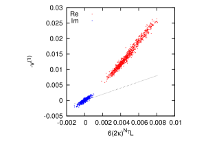
(a)

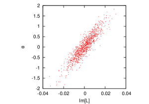
(b)

Figure 2: (a) Correlation between the the fuzzy Polyakov loop $-v^{(1)}$ and Polyakov loop $L$ multiplied with $6(2\kappa)^{N_{\text{t}}}$ on 1000 phase quenched configurations. Red and blue points respectively represent the real and imaginary part. The dotted black line shows the static limit for the fuzzy Polyakov loop given in Eq. (37). (b) correlation between the phase of determinant and the imaginary part of the Polyakov loop. The simulation parameters are as follows: $8^{3}\times 4$, $\beta=1.60$, $\kappa=0.1371$ and $a\mu=0.205$.

In Fig. 2 (a), we show the correlation between $-v^{(1)}$ and $6(2\kappa)^{N_{\text{t}}}L$. The real part as well as the imaginary part shows a strong correlation in the parameter space where we investigate, albeit the deviation from the static limit is significant.

As is seen from Eq. (15), the imaginary part of $v^{(q)}$ contributes to the phase of the determinant. Therefore a correlation between the phase and the imaginary part of the Polyakov loop is also expected. It is indeed confirmed in Fig. 2(b) where the phase is exactly computed from $W(\mu/T)\in\mathbb{C}$ in Eq. (12) up to $2\pi$ periodicity. Such a correlation was observed in Ref. de Forcrand and Laliena (2000) in the heavy mass region for the staggered quark action.

If the power of fugacity is promoted to an independent parameter for each $q\in\mathbb{Z}$,

$$e^{q\mu/T}\longrightarrow\lambda^{(q)},$$ (38)

$v^{(q)}$ can be considered as the first derivative of the promoted partition function $\mathcal{Z}_{\text{QCD}}$ in terms of the new parameter,

$$\langle v^{(q)}\rangle=-\frac{1}{N_{\text{f}}V}\left.\frac{\partial\ln\mathcal{Z}_{\text{QCD}}}{\partial\lambda^{(q)}}\right|_{\lambda^{(q)}=\exp(q\mu/T)},$$ (39)

with

$$\mathcal{Z}_{\text{QCD}}(..,\lambda^{(1)},\lambda^{(2)},\lambda^{(3)},...)=\int[\operatorname{d\!}U]\exp\left\{-S_{\text{G}}[U]+N_{\text{f}}\ln A_{0}-N_{\text{f}}V\sum_{q\in\mathbb{Z}}\lambda^{(q)}v^{(q)}\right\}.$$ (40)

In the end, we impose $\lambda^{(q)}=e^{q\mu/T}$ for all $q\in\mathbb{Z}$ to restore the original theory. Singularities of the theory may be captured by this quantity. Therefore we analyze higher cumulants of $v^{(q)}$ defined by taking higher derivatives of $\ln\mathcal{Z}_{\text{QCD}}$. In practice, we exclusively analyze the cumulants of $v^{(1)}$.

V.4 Quark number

The quark number density normalized by $T^{3}$ is given by

$$\frac{n_{\text{q}}}{T^{3}}=\frac{1}{VT^{3}}\frac{\partial\ln\mathcal{Z}_{\text{QCD}}}{\partial(\mu/T)}=\frac{\langle Q_{1}\rangle}{VT^{3}}.$$ (41)

Following the general definition adopted in Sec. V.1, the other higher moments are given by

$$\frac{\chi_{\text{q}}}{T^{2}} =\frac{1}{VT^{3}}(\ln\mathcal{Z}_{\text{QCD}})^{(2)}=\frac{\langle Q_{2}\rangle-\langle Q_{1}\rangle^{2}}{VT^{3}},$$ (42)

$$S_{\text{q}} =\frac{(\ln\mathcal{Z}_{\text{QCD}})^{(3)}}{((\ln\mathcal{Z}_{\text{QCD}})^{(2)})^{3/2}}=\frac{\langle Q_{3}\rangle-3\langle Q_{2}\rangle\langle Q_{1}\rangle+2\langle Q_{1}\rangle^{3}}{(\langle Q_{2}\rangle-\langle Q_{1}\rangle^{2})^{3/2}},$$ (43)

$$K_{\text{q}} =\frac{(\ln\mathcal{Z}_{\text{QCD}})^{(4)}}{((\ln\mathcal{Z}_{\text{QCD}})^{(2)})^{2}}=\frac{\langle Q_{4}\rangle-4\langle Q_{3}\rangle\langle Q_{1}\rangle-3\langle Q_{2}\rangle^{2}+12\langle Q_{2}\rangle\langle Q_{1}\rangle^{2}-6\langle Q_{1}\rangle^{4}}{(\langle Q_{2}\rangle-\langle Q_{1}\rangle^{2})^{2}},$$ (44)

where $(n)$ means the $n$-th derivative $\partial^{n}/\partial(\mu/T)^{n}$, $Q_{n}(n=1,2,3,4)$ are given in Eq. (19), and the CLB cumulant takes the form,

$$U_{\text{q}}=1-\frac{\langle Q_{4}\rangle}{3\langle Q_{2}\rangle^{2}}.$$ (45)

VI Simulation results

We now discuss simulation results for the expectation value, susceptibility and higher cumulants. In the figures we only plot their real part since their imaginary part vanishes due to symmetry.

VI.1 Numerical evaluation of $\mu$-reweighting

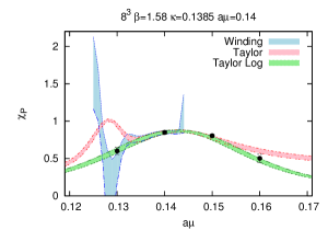
(a)

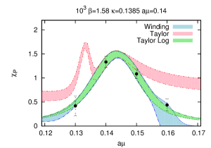
(b)

Figure 3: Comparison of three expansion schemes of $\mu$-reweighting for the susceptibility of plaquette. Winding expansion: blue band; Taylor expansion: red band; Taylor expansion of the logarithm of the determinant:green band. Black symbols are direct simulation data. The original $\mu$-value is $a\mu=0.14$. (a) $8^{3}\times 4$, (b) $10^{3}\times 4$.

In Fig. 3, we compare the three expansion schemes introduced in Sec. III, taking the susceptibility of plaquette for illustration. The starting value is $a\mu=0.14$, and the results of $\mu$-reweighting are shown by the one standard deviation error bands. The simulation paramaters are given in the figure. The performance of $\mu$-reweighting can be measured by comparison of the bands with actual measurements away from $a\mu=0.14$ plotted by filled circles. Comparing the results for $8^{3}\times 4$ lattice in (a) and for $10^{3}\times 4$ lattice in (b), we see that the winding expansion works better for larger volume. The Taylor expansion develops a fake transition around $a\mu=0.128$ on $8^{3}\times 4$ lattice and around $a\mu=0.133$ on $10^{3}\times 4$ lattice, respectively. The applicable range of $\mu$-reweighting for this expansion becomes smaller for larger volumes. In contrast to the two expansions, the Taylor expansion of the logarithm is working well for both lattice sizes and the applicable range is quite wide compared with the other expansion schemes.

A possible explanation of this behavior is as follows. As is seen from Eq.(20), the coefficients of Taylor expansion of the logarithm $W_{n}$ are made of single trace whose magnitude would be proportional to the reduced space, namely the spatial lattice size $W_{n}\propto V$. Since this holds for all $n=1,2,3,4,...$, the magnitude of $W_{n}$ would not increase for larger $n$. Such a tendency is observed in $\langle W_{n}\rangle_{||}$ as shown in Fig. 4. On the other hand, the coefficients of Taylor expansion $Q_{n}$ are made from a product of $W_{n}$. Hence the dominant volume scaling is expected to be $Q_{n}\propto V^{n}$, and this tendency is seen in Fig. 4. In this way, we conclude that the Taylor expansion of the logarithm of the determinant is the best among our choices. This expansion scheme is used in the following $\mu$-reweighting results.

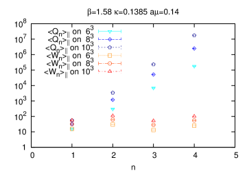
Figure 4: Phase quenched average of coefficients $Q_{n}$ and $W_{n}$ as a function of $n$. $Q_{n}$ are for the Taylor expansion of the determinant, and $W_{n}$ for the Taylor expansion of the logarithm of the determinant. The spatial volume is changed from $6^{3}$ to $10^{3}$ while the temporal lattice size is fixed to $N_{\text{t}}=4$. Error bars are too small to see at this scale.

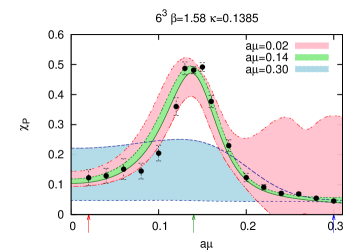
Figure 5: Comparison of the susceptibility of plaquette calculated from $\mu$-reweighting and from direct simulation. Black symbols show results from direct simulations. Colored regions show one standard deviation bands of $\mu$-reweighted results. Three different ensembles are used for $\mu$-reweighting, and their respective simulation points, $a\mu$, are labeled in the figure and also pointed at the horizontal axis by the same colored arrow

Lastly, we compare $\mu$-reweighting from ensembles at three original values of $\mu$ given by $a\mu=0.02$ and $0.14$ and $0.30$ in Fig. 5. The statistics for each ensemble are roughly the same order. We observe that the data reweighted from $a\mu=0.14$ shows an excellent agreement with the actual simulation data plotted by filled circles over a wide range from $a\mu=0.02$ to $0.30$. Also the estimated errors do not change much over this region. On the other hand, the reweighting from $a\mu=0.02$ and $0.30$ do not work well away from the original value. This may mean that not only the truncation error of the expansion but also the overlap issue is very important. The configurations generated at $a\mu=0.14$ are sampled from both low density phase and high density phase. Therefore the distribution of the plaquette has large overlaps with both phases. On the other hand, the configurations generated at $a\mu=0.02$ are mainly sampled from the low density phase, and hence the overlap with the high density phase region is very small. An opposite situation holds for the configurations generated at $a\mu=0.30$.

VI.2 Phase-reweighting factor

In Fig. 6 we show the phase-quenched average of the phase-reweighting factor as a function of $a\mu$ at $\beta=1.58$ and $1.60$. The $\mu$-reweighting one standard deviation error bands from $a\mu=0.14$ at $\beta=1.58$ and from $a\mu=0.205$ at $\beta=1.60$ are also shown. For larger volumes, the reweighting factor tends closer to zero, such that the sign problem becomes more serious as expected. However, since the phase-reweighting factor remains non-vanishing beyond statistical errors, the sign problem is under control for the lattice volumes and the parameter sets used in the present simulations.

An interesting observation is that there is a local minimum around $a\mu=0.14$ ($a\mu=0.2$) for $\beta=1.58$ ($\beta=1.60$). This is related to a change in the partition function, which usually appears as a consequence of a phase transition. It will be apparent when we discuss the behavior of the pressure in Sec. VI.10.

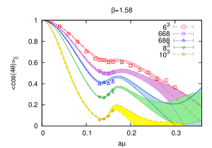
(a)

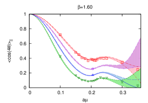
(b)

Figure 6: The phase-reweighting factor as a function of chemical potential at (a) $\beta=1.58$ and (b) $\beta=1.60$. The spatial volume is changed from $6^{3}$ to $10^{3}$ ($6^{3}$ to $8^{3}$) for $\beta=1.58$ ($\beta=1.60$). Filled curves show $1\sigma$ error band of the $\mu$-reweighed data from the original point at $a\mu=0.14$ and $0.205$ for $\beta=1.58$ and $1.60$ respectively.

VI.3 Comparison between QCD and phase-quenched QCD

Fig. 7 compares the average value of plaquette and the quark number density calculated with and without the phase of the quark determinant at $\beta=1.60$ on a $8^{3}\times 4$ lattice. Apart from a small difference resembling a shift in $a\mu$ in the region of rapidly increasing plaquette, the effect of inclusion of the phase is quite small in the figure for large values of $a\mu$. Such a trend is observed also for higher moments and other physical quantities. Similar observation has been reported in Ref. Sasai et al. (2004) in $N_{\text{f}}=2$ QCD by the phase reweighting method. In Ref. Hanada et al. (2012) it was argued that such a phenomena should hold at the parameter points outside of the charged pion condensation phase in the large $N_{c}$ limit.

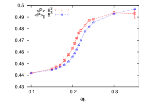
(a)

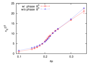
(b)

Figure 7: (a) Plaquette average and (b) quark number density as a function of $a\mu$ at $\beta=1.60$ on a $8^{3}\times 4$ lattice. Red squares are results for full QCD and blue triangles for phase-quenched QCD.

VI.4 Comparision with the Kentucky group

The Kentucky group Li et al. (2010) carried out a canonical simulation at $\beta=1.60$ and $\kappa=0.1371$ on a $6^{3}\times 4$ lattice employing the same gluon and quark actions as in the present study. In their work, the quark or baryon chemical potential $\mu_{\text{q}}=\mu_{\text{B}}/3$ is measured at fixed quark or baryon number $n_{\text{q}}=3n_{\text{B}}$, and they constructed an S-shape in their baryon number versus baryon chemical potential plot. In our grand canonical simulation, on the other hand, the input is the chemical potential and the output is the quark number. We numerically compare the two approaches in Fig. 8 for the same parameter set; filled symbols in (a) with vertical error bars are the canonical results from Fig. 7 (bottom) in Ref. Li et al. (2010), whereas open symbols in (b) with horizontal error bars are our grand canonical results.

Outside the transition region, say $n_{\text{B}}\leq 4$ and $n_{\text{B}}\geq 10$, results from the two approaches agree with each other. However, the two approaches show completely different behavior around the transition region. Graphically speaking in Fig. 8, while the canonical results can be made to produce an S-shape presumed from a first order transition, the grand canonical results are expected to show a smooth behavior and examination of higher cumulants such as susceptibility is required for an indication of a transition. The results of cumulant analyses, however, suggest a numerical difference: the Maxwell construction of the canonical results implies $\mu_{\text{B}}/T\approx 2.2$ at the transition, whereas the peak of quark number susceptibility from grand canonical results in this study takes place at $\mu_{\text{B}}/T\approx 2.5$. In principle the two approaches should lead to similar results if the infinite volume limit is taken carefully.

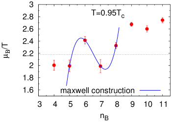
(a)

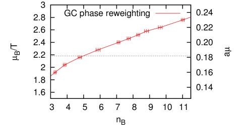
(b)

Figure 8: Comparison of canonical (filled circles in (a)) and grand canonical (open symbols in (b)) results for the relation between baryon chemical potential $\mu_{\text{B}}/T$ and baryon number $n_{\text{B}}$. Canonical results are from Ref.Li et al. (2010) by the Kentucky group. Simulation parameters are $\beta=1.60$, $\kappa=0.1371$ on a lattice of size $6^{3}\times 4$.

VI.5 Susceptibility

The susceptibility of plaquette $\chi_{P}$ and quark number density $\chi_{\text{q}}/T^{2}$ are shown in Fig 9. We plot not only the actual simulation data with error bars but also the one standard deviation $\mu$-reweighting band. We observe a clear volume dependence at $\beta=1.58$; the peak grows rapidly for larger volume. At $\beta=1.60$ the peak still grows with volume but the rate is much milder. The susceptibilities for gauge action density, Polyakov and fuzzy Polyakov loop also show similar tendency. Therefore it is likely that there is a phase transition at $\beta=1.58$ while the situation at $\beta=1.60$ requires further quantitative analyses.

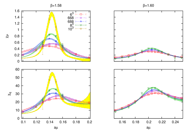
Figure 9: Susceptibility of plaquette (upper) $\chi_{P}$ and quark number density (lower) $\chi_{\text{q}}$ as functions of $a\mu$ at $\beta=1.58$ (left) and $\beta=1.60$ (right) for various spatial volumes.

We plot in Fig. 10 the volume dependence of the peak height of $\chi_{P}$ for (a) $\beta=1.58$ and (b) $\beta=1.60$. The peak position and the maximum value of $\chi_{P}$ is determined by the $\mu$-reweighting. The result for $\beta=1.58$ shows a clear linear volume dependence, while that for $\beta=1.60$ is rather weak.

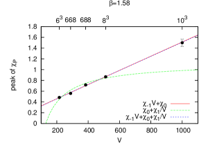
(a)

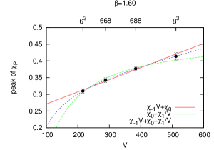
(b)

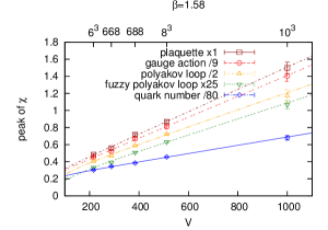
(c)

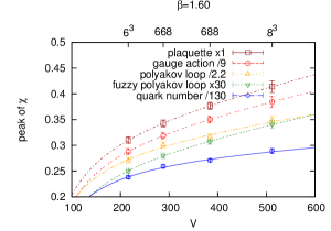
(d)

Figure 10: Upper panels show volume scaling of the peak value of $\chi_{P}$ for (a) $\beta=1.58$ and (b) $1.60$ together with three types of fits. Lower panels show volume scaling plots for all observables together with the fitting form S3 defined in the text. Vertical scales are adjusted.

To draw a quantitative conclusion, we first try a fitting of data with the functional form

$$\chi_{P}^{\max}=aV^{b}+c,$$ (46)

where $a$, $b$ and $c$ are fitting parameters. It turns out that for $\beta=1.58$ the exponent $b$ is consistent with 1 with a reasonable error bar and reduced $\chi^{2}$. On the other hand, the fit for $\beta=1.60$ is very unstable and it is difficult to obtain a meaningful exponent. In the following, we assume a volume dependence with integer powers of $V$ of the form

$$\chi_{P}^{\max}=\chi_{-1}V+\chi_{0}+\chi_{1}/V,$$ (47)

and consider three cases,

1. setting $\chi_{1}=0$

2. setting $\chi_{-1}=0$

3. no constraint

The results of the fits are summarized in Table 5 for $\beta=1.58$ and in Table 6 for $\beta=1.60$ for all susceptibilities we consider. In the bottom panels (c) and (d) in Fig. 10, the volume scaling behavior for all physical quantities are shown together with the fitting form S3.

Let us first look at Table 5. For all five observables, the fitting form S1 exhibits a reasonable reduced $\chi^{2}$, and the coefficient $\chi_{-1}$ is well determined and non-zero with less than a percent error. This situation holds even if one adds a $1/V$ term (fitting form S3), with the parameters $\chi_{-1}$ and $\chi_{0}$ keeping values consistent with those from the fitting form S1. In a sharp contrast, dropping the term linear in $V$ (fitting form S2) leads to an unacceptably large reduced $\chi^{2}$. We conclude that there is a first order phase transition at $\beta=1.58$.

At $\beta=1.60$ in Table 6, the fitting form S1 also provides a reasonable fit for all observables with a non-zero $\chi_{-1}$ at a 10% error level. However, the fitting form S2 without the term linear in volume also yields fits of similar quality. While a large negative coefficient $\chi_{1}$ of the $1/V$ term in the latter fit does not seem natural, we are not able to exclude such a possibility on other grounds. With present data alone, it is difficult to draw a clear distinction between a weak but first order phase transition and a crossover at $\beta=1.60$. Data for a larger spatial lattice volume, e.g., $10^{3}$, will help, but it seems very hard to accumulate enough statistics; the average of the fermion phase is already rather small for our largest spatial volume of $8^{3}$ (see Fig. 6).

Table 5: Fitted values of parameters and $\chi^{2}/{\text{dof}}$ in the volume scaling form of susceptibility in Eq. (47) for $\beta=1.58$. Values without errors are fixed during the fit.

observable	fitting form	$\chi_{-1}$	$\chi_{0}$	$\chi_{1}$	$\chi^{2}/{\text{dof}}$
	S1	$0.001318(53)$	$0.195(19)$	$0$	$0.853$
plaquette	S2	$0$	$1.130(22)$	$-147.1(6.4)$	$31.5$
	S3	$0.00130(14)$	$0.206(99)$	$-2(16)$	$1.27$
	S1	$0.01106(44)$	$1.65(16)$	$0$	$0.878$
gauge action	S2	$0$	$9.49(19)$	$-1231(53)$	$31.4$
	S3	$0.0110(11)$	$1.72(82)$	$-10(138)$	$1.31$
	S1	$0.002111(94)$	$0.353(33)$	$0$	$0.648$
Polyakov loop	S2	$0$	$1.816(38)$	$-224(11)$	$17.8$
	S3	$0.00199(28)$	$0.44(19)$	$-14(31)$	$0.866$
	S1	$0.0000400(14)$	$0.00466(48)$	$0$	$0.997$
fuzzy Polyakov loop	S2	$0$	$0.03258(59)$	$-4.29(16)$	$30.3$
	S3	$0.0000370(39)$	$0.0069(28)$	$-0.36(44)$	$1.18$
	S1	$0.0399(19)$	$15.74(74)$	$0$	$0.488$
quark number	S2	$0$	$45.04(75)$	$-4785(241)$	$23.5$
	S3	$0.0384(46)$	$17.0(3.5)$	$-216(600)$	$0.668$

Table 6: Fitted values of parameters and $\chi^{2}/{\text{dof}}$ in the volume scaling form of susceptibility for $\beta=1.60$.

observable	fitting form	$\chi_{-1}$	$\chi_{0}$	$\chi_{1}$	$\chi^{2}/{\text{dof}}$
	S1	$0.000362(39)$	$0.235(13)$	$0$	$0.497$
plaquette	S2	$0$	$0.472(14)$	$-35.8(3.9)$	$1.02$
	S3	$0.00022(15)$	$0.332(99)$	$-15(15)$	$0.00052$
	S1	$0.00302(33)$	$1.97(11)$	$0$	$0.546$
gauge action	S2	$0$	$3.95(12)$	$-299(33)$	$0.924$
	S3	$0.0017(13)$	$2.83(82)$	$-132(127)$	$7.32\times 10^{-7}$
	S1	$0.000555(72)$	$0.486(25)$	$0$	$1.03$
Polyakov loop	S2	$0$	$0.855(25)$	$-56.4(7.3)$	$1.07$
	S3	$0.00029(28)$	$0.67(18)$	$-28(28)$	$1.08$
	S1	$0.00001028(95)$	$0.00624(32)$	$0$	$0.714$
fuzzy Polyakov loop	S2	$0$	$0.01303(33)$	$-1.034(96)$	$1.47$
	S3	$0.0000062(36)$	$0.0090(24)$	$-0.43(37)$	$0.0651$
	S1	$0.0222(23)$	$26.63(79)$	$0$	$2.12$
quark number	S2	$0$	$41.49(81)$	$-2286(235)$	$0.801$
	S3	$0.0067(89)$	$37.1(5.9)$	$-1625(909)$	$1.03$

VI.6 Skewness

The skewness of plaquette and quark number density are shown in Fig. 11. The zero of the skewness yields an estimate of the transition point and the slope at the zero is expected to negatively increase with volume. The latter feature is apparent in Fig. 11. The zeros estimated by $\mu$-reweighting are consistent with the peak position of the susceptibility for each observable and volume. We find the volume dependence of the position of zero to be less than 10%.

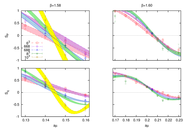
Figure 11: Skewness of plaquette $S_{P}$ (upper panels), and quark number density $S_{\text{q}}$ (lower panels) as functions of $a\mu$ at $\beta=1.58$ (left) and $\beta=1.60$ (right).

VI.7 Kurtosis

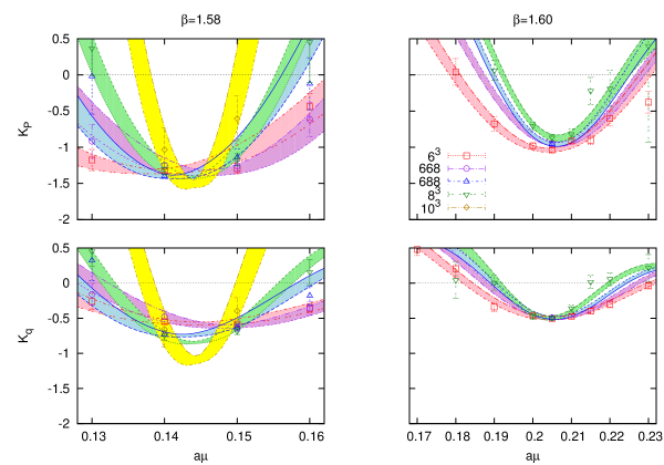
Figure 12: Kurtosis of plaquette $K_{P}$ (upper panels) and quark number density $K_{\text{q}}$ (lower panels) as functions of $a\mu$ at $\beta=1.58$ (left) and $\beta=1.60$ (right).

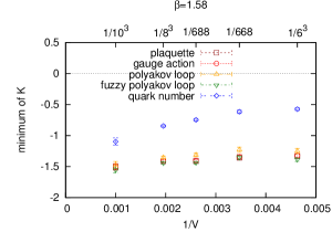
(a)

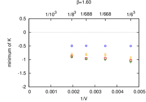
(b)

Figure 13: Volume scaling of the minimum value of the kurtosis for all physical quantities at (a) $\beta=1.58$ and (b) $\beta=1.60$.

The results of the kurtosis of plaquette and quark number density are plotted in Fig. 12. We observe a dip which becomes sharper for larger volumes. We also find that the peak position of the susceptibility and the position of the minimum of the kurtosis is consistent with each other for all physical quantities and each volume. These features are as expected from a simple double Gaussian model discussed in Appendix A.

Fig. 13 shows volume scaling of the minimum of kurtosis for all observables. At $\beta=1.58$, the minimum decreases for larger volumes. Infinite volume extrapolations assuming polynomials in $1/V$, however, do not yield values close to $-2$ expected for a first order phase transition. For $\beta=1.60$, the minimum shows only weak volume dependence, and even increases slightly for larger volumes.

Since kurtosis is composed of the fourth order cumulants, statistical errors are significantly larger compared to the second order cumulants (compare Fig. 9 and Fig. 12). Furthermore, the curvature at the minimum is expected to increase quadratically in $V$. Unless data at the original value is precise, $\mu$-reweighting may find hard time estimating the bottom of a sharp valley. We feel that these features make kurtosis a rather difficult quantity. We will need much more detailed analysis with larger statistics and/or finer points of simulations to draw definitive information from kurtosis.

VI.8 CLB cumulant

In Fig. 14, we show the CLB cumulant for plaquette $U_{P}$, quark number density $U_{\text{q}}$, and Polyakov loop $U_{L}$. Both $U_{P}$ and $U_{L}$ show a unique minimum in the region we investigate. The volume dependence of the minimum position is rather large for $U_{L}$ while it is small for $U_{P}$. The results for gauge action density and fuzzy Polyakov loop show similar trends to that of plaquette and Polyakov loop, respectively. In contrast, $U_{\text{q}}$ exhibits a broad minimum even for relatively large volumes, and there is an additional minimum generated far away from the transition region for large volumes. Since the CLB cumulant is defined in terms of non-central moments, it may depend more on the detailed form of observable distributions than those defined in terms of central moments and their ratios. In any case we need more understanding on the behavior of $U_{\text{q}}$, and we choose not to perform the volume scaling analysis for $U_{\text{q}}$ in the following.

Figure 14: CLB cumulant of plaquette $U_{P}$ (top panels), quark number density $U_{\text{q}}$ (middle panels), and the Polyakov loop $U_{L}$ (bottom panels) as functions of $a\mu$ at $\beta=1.58$ (left) and $\beta=1.60$ (right).

(a)

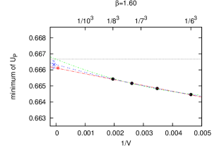
(b)

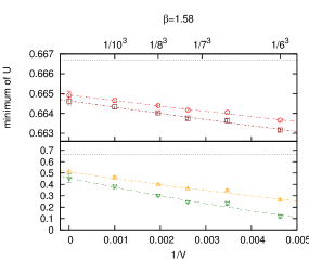
(c)

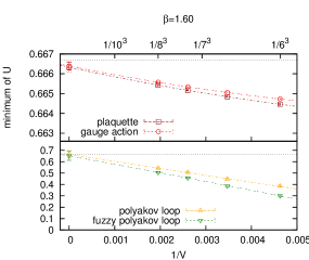
(d)

Figure 15: Upper panels show volume scaling of the minimum of $U_{P}$ for $\beta=1.58$ (left panel) and $1.60$ (right panel) together with results of three types of fits. Lower panels show volume scaling plot for plaquette, gauge action density, Polyakov loop, and fuzzy Polyakov loop, together with results of the fitting form C3.

In order to extract the infinite volume limit, we perform fitting with the form

$$U^{\min}_{P}=u_{0}(1-u_{1}/V+u_{2}/V^{2}),$$ (48)

and consider three cases,

1. assuming $u_{2}=0$

2. assuming $u_{0}=2/3$

3. no constraint

The results for fit parameters are summarized in Table 7 and 8 for $\beta=1.58$ and $1.60$, respectively. In Fig. 15, the top panels shows the volume dependence of the minimum value of the CLB cumulant for plaquette, together with the curves of the three fits. The bottoms panels summarize the minimum values for all observable we consider and the fit curves from the fitting form C3.

We find the results of fits to be essentially the same in character to those for the susceptibilities. At $\beta=1.58$, data are well described by either the fitting form C1 or C3, with consistent values of the fit parameters. In particular, $u_{0}$ clearly deviates away from $2/3$. On the other hand, the fitting form C2 with $u_{0}$ fixed at $2/3$ has an unacceptably large $\chi^{2}$. Thus a crossover is strongly excluded. At $\beta=1.60$, the fitting form C1 and C2 are equally reasonable. It is difficult to distinguish between a first order phase transition and a crossover from present data alone.

Table 7: Values of fit parameters of volume scaling form for CLB cumulant in Eq. (48) at $\beta=1.58$. Values without error means that the corresponding parameter is fixed.

observable	fitting form	$u_{0}$	$u_{1}$	$u_{2}$	$\chi^{2}/{\text{dof}}$
	C1	$0.664614(82)$	$0.462(44)$	$0$	$1.02$
plaquette	C2	$2/3$	$2.640(52)$	$342(15)$	$31.7$
	C3	$0.66463(21)$	$0.48(23)$	$4(38)$	$1.53$
	C1	$0.664901(74)$	$0.398(40)$	$0$	$0.742$
gauge action	C2	$2/3$	$2.258(46)$	$291(13)$	$26.3$
	C3	$0.66492(20)$	$0.42(22)$	$4(35)$	$1.11$
	C1	$0.499(12)$	$100.3(6.6)$	$0$	$1.39$
polyakov loop	C2	$2/3$	$255.6(7.4)$	$0.296(22)\times 10^{5}$	$10$
	C3	$0.511(30)$	$116(37)$	$0.30(71)\times 10^{4}$	$2$
	C1	$0.435(16)$	$153.5(8.3)$	$0$	$2$
fuzzy polyakov loop	C2	$2/3$	$353(10)$	$0.403(29)\times 10^{5}$	$12.1$
	C3	$0.455(38)$	$182(47)$	$0.61(99)\times 10^{4}$	$2.83$

Table 8: Values of fit parameters of volume scaling form for CLB cumulant at $\beta=1.60$.

observable	fitting form	$u_{0}$	$u_{1}$	$u_{2}$	$\chi^{2}/{\text{dof}}$
	C1	$0.666118(60)$	$0.545(30)$	$0$	$0.453$
plaquette	C2	$2/3$	$1.083(32)$	$81.2(8.9)$	$1.05$
	C3	$0.66633(23)$	$0.76(23)$	$33(35)$	$0.00105$
	C1	$0.666175(54)$	$0.478(27)$	$0$	$0.573$
gauge action	C2	$2/3$	$0.961(29)$	$73.0(8)$	$0.869$
	C3	$0.66639(21)$	$0.69(20)$	$33(31)$	$1.02\times 10^{-5}$
	C1	$0.6621(91)$	$91.3(3.7)$	$0$	$0.551$
polyakov loop	C2	$2/3$	$95.4(4.8)$	$0.08(15)\times 10^{4}$	$0.545$
	C3	$0.666(34)$	$95(30)$	$0.06(54)\times 10^{4}$	$1.09$
	C1	$0.656(11)$	$117.2(4)$	$0$	$0.164$
fuzzy polyakov loop	C2	$2/3$	$125.5(5.6)$	$0.15(17)\times 10^{4}$	$0.234$
	C3	$0.651(39)$	$112(34)$	$-0.10(65)\times 10^{4}$	$0.306$

VI.9 Transition point

The transition point can be determined by the peak of the susceptibility or the zero of the skewness for each volume. The transition point in the infinite volume may then be obtained by a volume extrapolation with a fitting form

$$a\mu_{\text{t}}(V)=a\mu_{\text{t}}(V=\infty)+A/V,$$ (49)

where $a\mu_{\text{t}}(V=\infty)$ and $A$ are fitting parameters. The volume dependence of the transition point determined from the susceptibility for five observables, and the volume extrapolation using Eq. (49), are shown in Fig. 16. The largest three volumes are used for the fits, namely $V=688,8^{3},10^{3}$ for $\beta=1.58$ and $V=668,688,8^{3}$ for $\beta=1.60$. The transition points determined from several observables are different from each other at finite volumes. However, after taking the infinite volume limit, they coincide with each other within the estimated errors. The transition point determined by the zero of skewness gives the same value within error at each finite volume, and the final value and the size of error are similar to those calculated from susceptibilities. For future reference we quote the transition point determined from the susceptibility of plaquette,

$$a\mu_{\text{t}}(V=\infty)=\left\{\begin{array}[]{cc}0.1459(20)&\mbox{ for }\beta=1.58,\\ 0.2053(21)&\mbox{ for }\beta=1.60.\\ \end{array}\right.$$ (50)

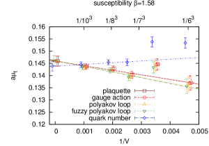
(a)

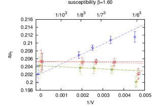
(b)

Figure 16: Volume dependence of the transition point $a\mu_{\text{t}}$ determined from susceptibility peak of several observables for (a) $\beta=1.58$ and (b) $1.60$ together with the fitted line of Eq. (49).

VI.10 Pressure

For the grand canonical ensemble approach, the pressure is given by the corresponding partition function,

$$p_{\text{QCD}}(\mu)=\frac{T}{V}\ln\mathcal{Z}_{\text{QCD}}(\mu).$$ (51)

The ratio of two partition functions is thus directly related to their difference in pressure. The averaged phase-reweighting factor, which is the ratio of full QCD partition function and phase-quenched partition function, can be expressed as the difference in pressure,

$$\langle\cos(4\theta)\rangle_{||}=\exp\left[\frac{V}{T}\left(p_{\text{QCD}}(\mu)-p_{\text{QCD}_{||}}(\mu)\right)\right]=\exp\left[\frac{V}{T}\Delta p(\mu)\right]\leq 1.$$ (52)

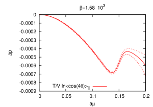
(a)

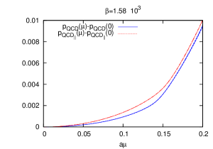
(b)

Figure 17: The left figure is the difference of the pressure between full QCD and phase quenched QCD with $1\sigma$ error band. The right figure is the subtracted pressure for QCD and phase quenched QCD as a function of $a\mu$ at $\beta=1.58$ on $10^{3}$ lattice. The inequality $p_{\text{QCD}}(\mu)\leq p_{\text{QCD}_{||}}(\mu)$ in the shown range of $\mu$ is seen. The pressure here is in lattice unit.

Conversely, the pressure difference between full QCD and phase-quenched is given by $T/V\ln\langle\cos(4\theta)\rangle_{||}$, and is shown in Fig. 17(a). This can be compared with Fig. 6, where the dip in the phase-reweighting factor manifests itself as the dip in the pressure difference. In order to better understand the local minimum, we compare the pressure from full QCD and phase-quenched directly by plotting them together in Fig. 17(b). In this figure, we show the value of each pressure at chemical potential, $\mu$, relative to the value at $\mu=0$. These are computed by numerically integrating the quark number density (Eq. (41)),

$$p(\mu)-p(0) =\frac{T}{V}\int_{0}^{\mu}d\mu^{\prime}\frac{\partial\ln\mathcal{Z}(\mu^{\prime})}{\partial\mu^{\prime}},$$ (53)

$$=\int_{0}^{\mu}d\mu^{\prime}n_{\text{q}}(\mu^{\prime}).$$ (54)

We can see, in Fig. 17, that there is a change of slope in full QCD appears at a relative smaller chemical potential than the change of slope in phase-quenched QCD does. This produces the dip.

The slope in figures of pressure versus chemical potential is quark number density as given in Eq. (54). The rapid increase of slope here is the same as a rapid increase of quark number density, which is an expected behavior for a phase transition. Fig. 18 shows results of relative pressure in full QCD from our simulations. Compared to our moment analysis, at $\beta=1.58$, where the first order phase transition is suggested, the slope around the transition point ($a\mu\approx 0.146$) changes more rapidly with larger volumes and it is likely to develop a discontinuity in the first derivative of pressure in the infinite volume limit, which is a classical signal of a first order phase transition. On the other hand, at $\beta=1.60$ with the volumes we have simulated, the change is less sharp, which is consistent with results from other moments, namely a crossover.

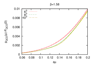
(a)

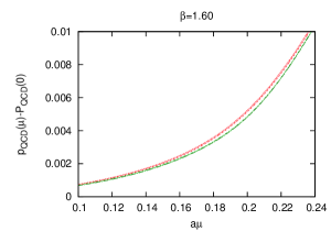
(b)

Figure 18: The left (right) figure is the subtracted pressure as a function of $a\mu$ at $\beta=1.58$ ($1.60$). The band shown here is 1 $\sigma$-band.

Finally, after understanding the meaning of the first derivative of pressure, the dip in Fig. 17(a) can be explained in the following way. It appears when the first derivative of pressure in full QCD changes more rapidly than that in phase-quenched. When the phase-quenched system is away from a transition while the full QCD system undergoes a transition, such dip becomes sharper. The dip becomes a downward wedge—a discontinuity in slope—in the thermodynamic limit, when a first order transition occurs.

VII Global picture of phase diargram

We may ask what present results can tell us about the phase diagram depicted in Fig. 1. To answer this question we made additional simulations at $a\mu=0$ with $(\beta,\kappa)=(1.600,0.1380)$ and $(1.618,0.1371)$. The volume scaling of the histogram for the gauge action density and the susceptibility and the CLB cumulant shown in Fig. 19 indicate that the former point has a clear first order phase transition, while the latter point has a much weaker transition, possibly consistent with a crossover. Linearly connecting the two points yields $\kappa_{\text{t}}\approx 0.2180-0.0500\beta$ as an estimate of the line of transition. Since we wish to draw the phase diagram for a fixed quark mass in physical units, we calculate $m_{\pi}/m_{\rho}$ from Table 3, and find $m_{\pi}/m_{\rho}\approx 0.555\beta-0.064$ along the line of transition. Given $m_{\pi}/m_{\rho}=0.822(3)$ also from Table 3, we estimate that the first order transition at $(\beta,\kappa,a\mu)=(1.58,0.1380,0.1459(20))$ is connected to the point $(1.596,0.1382,0)$ where we expect a first order transition from the zero density runs discussed above. We come to the conclusion that for $m_{\pi}/m_{\rho}=0.822(3)$ the phase diagram looks like Fig. 1(a).

A similar estimate starting from $(1.60,0.1371,0.2053(21))$ where $m_{\pi}/m_{\rho}=0.839(2)$ indicates that this point is connected to $(1.627,0.1367,0)$ where the transition is either a weak first order or a crossover. There is a possibility that the phase diagram looks like Fig. 1(b).

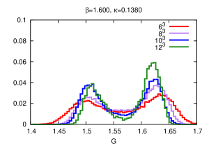
(a)

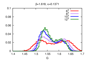
(b)

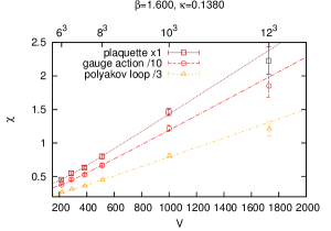
(c)

(d)

(e)

(f)

Figure 19: The top figure is the normalized histogram of the gauge action density. The left figures are for $\beta=1.600$ and $\kappa=0.1380$ while the right figures are for $\beta=1.618$ and $\kappa=0.1371$. The middle and the bottom figures show the volume scaling of susceptibility and the CLB cumulant respectively for the plaquette, the gauge action density and the Polyakov loop. In the bottom figures, the CLB cumulant of the Polyakov loop is not shown because its minimum is quite far from the simulation point. The curves show the fitting forms S3 and C3 defined in the Sec. VI.

VIII Concluding remarks

Taken together, the results of our finite size scaling analyses show that there is a first order phase transition at $\beta=1.58$, $\kappa=0.1380$ and $a\mu=0.1459(20)$. On the other hand, for the Kentucky group’s parameter set $\beta=1.60$, $\kappa=0.1371$, our range of lattice sizes from $6^{3}$ to $8^{3}$ is not large enough to draw a clear conclusion about the nature of the transition, although we have confirmed that the transition point $a\mu_{\text{t}}\approx 0.2053(21)$ is very close to that determined by their canonical approach.

Together with additional zero density simulations, we come to the conclusion that for $m_{\pi}/m_{\rho}=0.822(3)$ the phase diagram looks like Fig. 1(a). On the other hand, $m_{\pi}/m_{\rho}=0.839(2)$ indicates that the tansition is either a weak first order or a crossover and there is a possibility that the phase diagram looks like Fig. 1(b).

Appendix A Volume scaling of higher moments in a double Gaussian model

In this appendix, we summarize a phenomenological distribution argument originally due to Ref. Challa et al. (1986). Close to a first order transition point, the distribution of an observable $X$ can be approximately described by a double Gaussian form given by

$$P(X)=a_{+}\sqrt{\frac{V}{2\pi c_{+}}}e^{-\frac{(X-x_{+})^{2}}{2c_{+}/V}}+a_{-}\sqrt{\frac{V}{2\pi c_{-}}}e^{-\frac{(X-x_{-})^{2}}{2c_{-}/V}}.$$ (55)

This distribution is normalized

$$\int^{\infty}_{-\infty}P(X)dX=1,$$ (56)

provided $a_{+}+a_{-}=1$. Any observable $f(X)$ of $X$ can be calculated as

$$\langle f(X)\rangle=\int_{-\infty}^{\infty}\operatorname{d\!}Xf(X)P(X).$$ (57)

Let $t$ be the parameter controlling the phase transition, e.g., temperature, and let $a_{+}=a_{-}=1/2$ or $t=0$ be the transition point at infinite volume. The infinite volume free energy density has two branches which cross at $t=0$, and switches the minimum. Normalizing the scale of $t$, one can write

$$a_{\pm}=\frac{e^{\pm Vt}}{e^{Vt}+e^{-Vt}}.$$ (58)

Simple but tedius calculation leads to the following expressions for the susceptibility, skewness, kurtosis, and the CLB cumulant:

$$\chi_{X} =V\langle(X-\langle X\rangle)^{2}\rangle=Va_{+}a_{-}(x_{+}-x_{-})^{2}+(a_{+}c_{+}+a_{-}c_{-}),$$ (59)

$$S_{X} =\frac{\langle(X-\langle X\rangle)^{3}\rangle}{\langle(X-\langle X\rangle)^{2}\rangle^{3/2}}=-\frac{a_{+}-a_{-}}{\sqrt{a_{+}a_{-}}}+O(V^{-1}),$$ (60)

$$K_{X} =\frac{\langle(X-\langle X\rangle)^{4}\rangle}{\langle(X-\langle X\rangle)^{2}\rangle^{2}}-3=-2+\frac{1-4a_{+}a_{-}}{a_{+}a_{-}}+O(V^{-1}),$$ (61)

$$U_{X} =1-\frac{1}{3}\frac{\langle X^{4}\rangle}{\langle X^{2}\rangle^{2}}=\frac{2}{3}-\frac{a_{+}a_{-}(x_{+}^{2}-x_{-}^{2})^{2}}{3(a_{+}x_{+}^{2}+a_{-}x_{-}^{2})^{2}}+O(V^{-1}).$$ (62)

Another simple calculation of derivative with respect to $t$ leads to

$$\frac{d\chi_{X}}{dt} =-b(a_{+}-a_{-})(x_{+}-x_{-})^{2}V^{2}+b(c_{+}-c_{-})V,$$ (63)

$$\frac{dS_{X}}{dt} =-\frac{b}{2(a_{+}a_{-})^{3/2}}V+O(V^{0}),$$ (64)

$$\frac{dK_{X}}{dt} =-b\frac{a_{+}-a_{-}}{(a_{+}a_{-})^{2}}V+O(V^{0}),$$ (65)

$$\frac{dU_{X}}{dt} =\frac{b}{3}\frac{(a_{+}x_{+}^{2}-a_{-}x_{-}^{2})}{(a_{+}x_{+}^{2}+a_{-}x_{-}^{2})^{3}}(x_{+}^{2}-x_{-}^{2})^{2}V+O(V^{0}),$$ (66)

with $b=2/(e^{Vt}+e^{-Vt})$.

From the above equations, we read that the peak of susceptibility, zero of skewness and minimum of kurtosis take place at the same value $t=0$ up to corrections of $O(V^{-2})$. Expanding the skewness and kurtosis in the leading orders of $V$ around $t=0$ with $Vt\ll 1$, we find

$$S_{X} =-2Vt+O(V^{0}),$$ (67)

$$K_{X} =-2+4V^{2}t^{2}+O(V^{1}).$$ (68)

Therefore, in the leading order, the slope of skewness increases linearly, and the curvature of kurtosis quadratically, with volume.

The CLB cumulant exhibits a subtlety. The minimum position deviates from $t=0$ by $O(V^{-1})$:

$$t_{\text{CLB min}}=\frac{1}{2V}\ln\frac{x_{-}^{2}}{x_{+}^{2}}+O(V^{-2})$$ (69)

The infinite volume values at this minimum and at $t=0$ differ:

$$\left.U_{X}\right|_{t=t_{\text{CLB min}}} =\frac{2}{3}-\frac{(x_{+}^{2}-x_{-}^{2})^{2}}{12x_{+}^{2}x_{-}^{2}}+O(V^{-1}),$$ (70)

$$\left.U_{X}\right|_{t=0} =\frac{2}{3}-\frac{(x_{+}^{2}-x_{-}^{2})^{2}}{3(x_{+}^{2}+x_{-}^{2})^{2}}+O(V^{-1}).$$ (71)

This may seem paradoxical that $\lim_{V\rightarrow\infty}t_{\text{CLB min}}=0$, while $\lim_{V\rightarrow\infty}\left.U_{X}\right|_{t=t_{\text{CLB min}}}\neq\left.U_{X}\right|_{t=0}$. This is because, at the minimum of the CLB cumulant, $\lim_{V\rightarrow\infty}\frac{a_{+}}{a_{-}}=\frac{x_{-}^{2}}{x_{+}^{2}}$, which is away from unity where the phase transition occurs even in the infinite volume limit.

Appendix B Remark on $\mu$-reweighting for quark number related quantities

Note that the observables, like plaquette value, gauge action, Polyakov loop, fuzzy Polyakov loop are independent of $\mu$, while the quark number density has an explicit $\mu$-dependence. Therefore we have to identify a difference in the observable

$$\mathcal{O}(\mu^{\prime})=\mathcal{O}(\mu)+\Delta\mathcal{O}(\mu^{\prime},\mu).$$ (72)

Before identifying the difference, first let us remind the quark number related quantities. Actually, they can be expressed by using $Q_{n}$ in Eq. (19) as follows. In order to construct the quark number related observable at $\mu^{\prime}$ we have to know $Q_{n}(\mu^{\prime})$. For that purpose, we have to know $W_{n}(\mu^{\prime}/T)$ as seen from Eq. (19).

$$W_{n}(\mu^{\prime}/T)=W_{n}(\mu/T)+\Delta W_{n}(\mu^{\prime}/T,\mu/T).$$ (73)

There are two ways to approximate $\Delta W_{n}(\mu^{\prime}/T)$, namely the winding expansion and the Taylor expansion. In the following we show only the latter and it is given by

$$W_{n}(\mu^{\prime}/T) =\sum_{m=0}^{\infty}\frac{(\mu^{\prime}/T-\mu/T)^{m}}{m!}\frac{\partial^{m}W_{n}(\mu/T)}{\partial(\mu/T)^{m}}$$

$$=\sum_{m=0}^{\infty}\frac{(\mu^{\prime}/T-\mu/T)^{m}}{m!}W_{n+m}(\mu/T),$$ (74)

where we have used a relation

$$\frac{\partial^{m}W_{n}}{\partial(\mu/T)^{m}}=W_{n+m}.$$ (75)

We truncate the expansion up to $m=3$ and their explicit forms for $n=1,2,3,4$ are given by

$$W_{1}(\mu^{\prime}/T) =W_{1}+(\mu^{\prime}/T-\mu/T)W_{2}+\frac{(\mu^{\prime}/T-\mu/T)^{2}}{2}W_{3}+\frac{(\mu^{\prime}/T-\mu/T)^{3}}{3!}W_{4},$$ (76)

$$W_{2}(\mu^{\prime}/T) =W_{2}+(\mu^{\prime}/T-\mu/T)W_{3}+\frac{(\mu^{\prime}/T-\mu/T)^{2}}{2}W_{4}+\frac{(\mu^{\prime}/T-\mu/T)^{3}}{3!}W_{5},$$ (77)

$$W_{3}(\mu^{\prime}/T) =W_{3}+(\mu^{\prime}/T-\mu/T)W_{4}+\frac{(\mu^{\prime}/T-\mu/T)^{2}}{2}W_{5}+\frac{(\mu^{\prime}/T-\mu/T)^{3}}{3!}W_{6},$$ (78)

$$W_{4}(\mu^{\prime}/T) =W_{4}+(\mu^{\prime}/T-\mu/T)W_{5}+\frac{(\mu^{\prime}/T-\mu/T)^{2}}{2}W_{6}+\frac{(\mu^{\prime}/T-\mu/T)^{3}}{3!}W_{7}.$$ (79)

We approximate $W_{5}=W_{7}=\operatorname{tr}[B]$ and $W_{6}=\operatorname{tr}[C]$. The error of this approximation is suppressed by $(\Delta\mu/T)^{n}/n!$, and is relatively unnoticeable compared to the statistical error.

In this way, we obtain the difference $\Delta W_{n}(\mu^{\prime}/T,\mu/T)$ and then from this one can construct the difference of any quark number related observable.

References

- Fodor and Katz (2002) Z. Fodor and S. Katz, Phys.Lett. B534, 87 (2002), arXiv:hep-lat/0104001 [hep-lat] .
- D’Elia and Lombardo (2003) M. D’Elia and M.-P. Lombardo, Phys.Rev. D67, 014505 (2003), arXiv:hep-lat/0209146 [hep-lat] .
- Kratochvila and de Forcrand (2006) S. Kratochvila and P. de Forcrand, PoS LAT2005, 167 (2006), arXiv:hep-lat/0509143 [hep-lat] .
- Fukugita et al. (1990a) M. Fukugita, H. Mino, M. Okawa, and A. Ukawa, Phys.Rev.Lett. 65, 816 (1990a).
- Iwasaki et al. (1996) Y. Iwasaki, K. Kanaya, S. Sakai, and T. Yoshie, Z.Phys. C71, 337 (1996), arXiv:hep-lat/9504019 [hep-lat] .
- Takeda et al. (2012a) S. Takeda, Y. Kuramashi, and A. Ukawa, Phys.Rev. D85, 096008 (2012a), arXiv:1111.6363 [hep-lat] .
- Danzer and Gattringer (2008) J. Danzer and C. Gattringer, Phys. Rev. D78, 114506 (2008), arXiv:0809.2736 [hep-lat] .
- Nagata and Nakamura (2010) K. Nagata and A. Nakamura, Phys.Rev. D82, 094027 (2010), arXiv:1009.2149 [hep-lat] .
- Li et al. (2010) A. Li, A. Alexandru, K.-F. Liu, and X. Meng, Phys.Rev. D82, 054502 (2010), arXiv:1005.4158 [hep-lat] .
- Takeda et al. (2012b) S. Takeda, X.-Y. Jin, Y. Kuramashi, Y. Nakamura, and A. Ukawa, PoS LATTICE2012, 066 (2012b), arXiv:1211.2508 [hep-lat] .
- (11) Y. Iwasaki, University of Tsukuba Report No. UTHEP-118, 1983 (unpublished) .
- Ferrenberg and Swendsen (1989) A. M. Ferrenberg and R. H. Swendsen, Phys.Rev.Lett. 63, 1195 (1989).
- Aoki et al. (2006) S. Aoki et al. (CP-PACS Collaboration, JLQCD Collaboration), Phys.Rev. D73, 034501 (2006), arXiv:hep-lat/0508031 [hep-lat] .
- Nakamura and Stuben (2010) Y. Nakamura and H. Stuben, PoS LATTICE2010, 040 (2010), arXiv:1011.0199 [hep-lat] .
- Sexton and Weingarten (1992) J. Sexton and D. Weingarten, Nucl.Phys. B380, 665 (1992).
- Takaishi and de Forcrand (2006) T. Takaishi and P. de Forcrand, Phys.Rev. E73, 036706 (2006), arXiv:hep-lat/0505020 [hep-lat] .
- Fukugita et al. (1990b) M. Fukugita, M. Okawa, and A. Ukawa, Nucl.Phys. B337, 181 (1990b).
- Challa et al. (1986) M. S. Challa, D. Landau, and K. Binder, Phys.Rev. B34, 1841 (1986).
- de Forcrand and Laliena (2000) P. de Forcrand and V. Laliena, Phys.Rev. D61, 034502 (2000), arXiv:hep-lat/9907004 [hep-lat] .
- Sasai et al. (2004) Y. Sasai, A. Nakamura, and T. Takaishi, Nucl.Phys.Proc.Suppl. 129, 539 (2004), arXiv:hep-lat/0310046 [hep-lat] .
- Hanada et al. (2012) M. Hanada, Y. Matsuo, and N. Yamamoto, Phys.Rev. D86, 074510 (2012), arXiv:1205.1030 [hep-lat] .