A Bayesian Approach to Deriving Ages of Individual Field White Dwarfs

Abstract

We apply a self-consistent and robust Bayesian statistical approach to determining the ages, distances, and ZAMS masses of 28 field DA white dwarfs with ages of approximately 4 to 8 Gyrs. Our technique requires only quality optical and near-IR photometry to derive ages with $<$ 15% uncertainties, generally with little sensitivity to our choice of modern initial-final mass relation. We find that age, distance, and ZAMS mass are correlated in a manner that is too complex to be captured by traditional error propagation techniques. We further find that the posterior distributions of age are often asymmetric, indicating that the standard approach to deriving WD ages can yield misleading results.

1. Introduction

Age is one of the most fundamental of all stellar properties, yet it is far more difficult to determine age precisely than the other fundamental properties such as stellar mass, surface temperature, and luminosity. In part, this is because we determine age via indirect means that require us to first collect more directly observable quantities. But there is another major impediment; we can usually only measure age for an aggregate or system of stars. For example, the most common method of measuring stellar ages—fitting stellar isochrones to cluster photometry—requires that we obtain photometry for hundreds or thousands of stars in order to derive a single age for the entire system. We generally cannot precisely fit isochrones to single stars unless these stars are in rare stages of their evolution, such as just leaving the main sequence. Even in this case, we require exquisite distances and probably independently-determined stellar masses (e.g., from double-lined eclipsing binaries, Grundahl et al. 2008) to derive a precise age. The other major technique for measuring stellar ages—fitting white dwarf cooling models to the white dwarf luminosity function (WDLF)—also requires groups of stars. This technique has been used to derive an upper age limit to the Galactic disk (Winget et al. 1987; Oswalt et al. 1996; Leggett, Ruiz, & Bergeron 1998; Knox, Hawkins, & Hambly 1999) and to derive the ages of open and globular clusters (Claver 1995; von Hippel, Gilmore, & Jones 1995; Richer et al. 1998; von Hippel & Gilmore 2000; Kalirai et al. 2001; Andreuzzi et al. 2002; Hansen et al. 2004; 2007; Garcia-Berro et al. 2010). Yet, if we could reliably determine ages for individual field stars, we could more readily determine the onset of star formation in each of the Galactic stellar populations.

In this paper, we focus on determining ages for individual WDs. The technique for deriving individual WD ages was advanced by Bergeron, Leggett, & Ruiz (2001), who plotted WD mass versus $T_{\rm eff}$ for WDs and compared them to WD cooling models to derive individual stellar ages. Their version of this technique requires accurate WD masses ($\sigma_{M}\leq$ 0.1 M_☉) and temperatures ($\sigma_{T}\approx 150$ K) from spectroscopy for the warm WDs with Balmer lines or from precise parallaxes ($\sigma_{\pi}\leq$ 10%) for the cool WDs. Bergeron et al. were able to derive individual stellar ages precise to $\sim$1 Gy for WDs with mass $>$ 0.6 M_☉. For WDs with mass $<$ 0.6 M_☉, WD ages are degenerate. This now-standard technique relies on measuring $T_{\rm eff}$ from photometry or spectroscopy and log(g) from spectroscopy or WD surface area from trigonometric parallax. Because WDs have a mass-radius relation (Hamada & Salpeter 1961), either log(g) or surface area yield mass, and the mass and $T_{\rm eff}$, when compared to a WD cooling model, yield the WD cooling age. The WD mass is relied upon again to infer its precursor mass through the imprecisely-known initial-final mass relation (IFMR), which is the mapping from masses on the zero age main sequence (ZAMS) to WD masses. The precursor mass is then converted to a pre-WD lifetime via stellar evolution models (see Salaris et al. 2009, for a list of models often used). Finally, the precursor lifetime is added to the WD cooling age to determine the total age of the WD.

The technique we have just outlined has its advantages and disadvantages. The foremost advantage is that it yields reasonably precise ages for individual WDs. Secondarily, for cool WDs with masses $\geq$ 0.7 M_☉, the progenitor lifetime is short relative to the WD cooling age, and therefore uncertainties in the IFMR are unimportant (see, for instance, von Hippel et al. 2006, fig 16). On the negative side, this age technique involves many steps, some of which are typically performed inconsistently. For example, Salaris et al. (2009) detailed how current IFMRs may be constructed from an inconsistent set of isochrones or the subsequent analysis may not use the same isochrones as those used in the IFMR. The IFMR itself is determined via WDs in star clusters. Researchers can reliably deduce the WD masses from spectroscopic log(g) measurements (e.g., Salaris et al. 2009; Williams, Bolte, & Koester 2009), but determining their precursor masses is model-dependent. That model-dependent path requires researchers to fit the main sequence turn-off with model isochrones to derive the cluster age, subtract the WD cooling ages from the total cluster age, derive precursor lifetimes, and then infer the precursor masses from the same stellar evolution models. Yet most IFMR studies measure the WD masses and collect the cluster ages from the literature, thereby using a heterogeneous mix of stellar evolution models (see criticisms in Salaris et al. 2009) to infer precursor masses. This heterogeneous mix of stellar evolution models may or may not include the model set that any subsequent researchers use to estimate a precursor lifetime for their analysis of the age of an individual WD. An additional negative to determining WD ages via this process is that one has to correctly propagate errors through many steps. Some errors may start out symmetrically distributed (e.g., $T_{\rm eff}$), but we will show that the assumptions behind the standard propagation of errors are not met, casting doubt on the estimates and errors that they produce.

Our goal in this paper is to improve upon the current step-wise and often internally inconsistent approach to obtaining individual WD ages. We accomplish this by applying the first model-based statistical analysis that simultaneously fits WD photometry to models that combine stellar precursor evolution, the IFMR, WD cooling, and WD atmospheres.

Our Bayesian statistical approach allows us to combine external information, e.g., distances from trigonometric parallaxes or spectroscopic metallicities, with stellar photometry in order to calculate not only reliable fitted values of stellar parameters, but also the entire posterior distribution for each parameter, including error bars and correlations among parameters.

2. Observations of Hydrogen Atmosphere Field WDs

Our technique can be applied to any WD for which we know the atmosphere type and for which we have reliable models. As a first test of our technique, we sought a homogeneous sample of old H-atmosphere (DA) WDs with optical and near-IR photometry. DAs are the most common (Kleinman et al. 2004) and well-studied WDs, so they were a good starting point. The 28 DAs with optical and near-IR photometry published by Kilic et al. (2010) fit our needs. Kilic et al. selected 130 WDs from the large sample of Harris et al. (2006) by targeting all WDs with bolometric magnitudes greater than 14.6 and tangential velocities greater than 20 km s^-1, the goal of which was to create a clean sample of intrinsically faint and therefore old WDs. Kilic et al. (2010) measured $JHK$ photometry for 126 stars in this SDSS sample using the Near Infra-Red Imager and Spectrometer on Gemini-North, the 0.8-5.4 micron medium-resolution spectrograph and imager on the Infrared Telescope Facility, and the Wide-Field Camera on the United Kingdom Infra-Red Telescope. Their typical photometric error was 0.04 mag. Although SDSS $u$ photometry is also available for these stars, because the WD models we use (see below) did not fully incorporate the red wing of the Lyman $\alpha$ line (Kowalski & Saumon 2006; Rohrmann, Althaus, & Kepler 2011), we chose not to incorporate these $u$-band data in our analyses.

Some of the cooler WDs in the Kilic et al. (2010) sample are undoubtedly DAs, but they are too cool to excite Balmer lines, so their spectral type is currently unknown. Because our goal is to present our Bayesian technique and outline its capabilities, we put off to a subsequent paper the analysis of He-atmosphere (DB) WDs and WDs of uncertain spectral type. The data we analyze therefore consists of $grizJHK$ photometry from Kilic et al. for 28 DA WDs.

3. Statistical Method

We have developed a Bayesian approach to fitting isochrones to stellar photometry (von Hippel et al. 2006; DeGennaro et al. 2009; van Dyk et al. 2009; Stein et al. 2013). We term our software package BASE-9 for Bayesian Analysis of Stellar Evolution with 9 Parameters. BASE-9 compares stellar evolution models (listed below) to photometry in any combination of photometric bands for which there are data and models. BASE-9 was designed to analyze star clusters and accounts for individual errors for every data point, ancillary data such as cluster membership probabilities from proper motions or radial velocities, cluster distance (e.g., from Hipparcos parallaxes or the moving cluster method), cluster metallicity from spectroscopic studies, and it can incorporate information such as individual stellar mass estimates from dynamical studies of binaries or spectroscopic atmospheric analyses of WDs. BASE-9 uses a computational technique known as Markov chain Monte Carlo to derive the Bayesian joint posterior probability distribution for six parameter categories (cluster age, metallicity, helium content, distance, and reddening, and optionally a parametrized IFMR) and brute-force numerical integration for three parameter categories (stellar ZAMS mass, binarity, and cluster membership). The last three of these parameter categories include one parameter per star whereas the first six parameter categories refer to the entire cluster. As a result, for star clusters BASE-9 actually fits hundreds or thousands of parameters (= 3 N_star + 6) simultaneously. While we cannot constructively apply BASE-9 to individual main sequence stars, we can profitably apply BASE-9 to individual WDs because WDs have a mass-radius relation that constrains WD luminosity. In many cases, this constraint is sufficient to yield useful WD ages. We provide further details on our statistical method and computational techniques in the appendix.

We used BASE-9 to fit model WD spectral energy distributions (SEDs) to the observed $grizJHK$ photometry for 28 DAs. BASE-9 generates model SEDs by combining the following ingredients: stellar evolution models for the main sequence through the asymptotic giant branch stage (Girardi et al. 2000; Yi et al. 2001; or Dotter et al. 2008), an IFMR (Weidemann 2000; Williams et al. 2009; or one of two from Salaris et al. 2009), WD interior cooling models (Montgomery et al. 1999; Renedo et al. 2010), and WD atmosphere models (Bergeron et al. 1995). The precursor stellar evolution models affect our estimate of the length of time that a star spends evolving prior to becoming a WD through the well-known strong dependence on mass and weak dependence on stellar abundance. Each of these three stellar evolution models show only minor differences in precursor ages over the parameter ranges we explore.

Because our statistical model is Bayesian, we can take advantage of prior information, where available, to constrain parameters. For this problem, the results are insensitive to the precise choice of reasonable priors; details are given in the appendix. For stellar abundances, we assume that all of these WDs are Galactic disk stars that started out with solar-ratio abundances and a Gaussian distribution for metallicity, [Fe/H] = 0.0 $\pm$ 0.3. This is reasonable because these stars display disk proper motions (Kilic et al. 2010). Additionally, stellar abundances change the properties of WDs only through slight changes to the precursor lifetimes (see discussion below). Because of the high surface gravities of WDs, their primordial abundances are not reflected in their atmospheres (Dupuis et al. 1992; Koester & Wilken 2006) and those WDs that are metal-polluted (spectral type DZ, DAZ, or DBZ) are actively accreting from their circumstellar environment (e.g., Jura 2003; von Hippel et al. 2007; Farihi et al. 2010). We do not include DZ-type WDs in this analysis. We set a Gaussian prior on distance modulus, $m-M$ = 4.0 $\pm$ 2.5, equivalent to $63\pm^{136}_{43}$ pc. Our distance prior is so loose that it does not constrain the results. It is included only because a prior on every parameter is required by the Bayesian approach. We impose a strict prior on absorption, $A_{\rm V}$ = 0. This absorption prior may be in error by a few thousandths of a mag, but all of these stars are nearby, typically $<$ 100 pc, and out of the Galactic plane, so the absorption is essentially zero.

Besides our primary goal of developing a simultaneously consistent and statistically robust method to derive ages for individual WDs, we set a secondary goal of checking the sensitivity of WD ages to the IFMR. This sensitivity has been largely unexplored, yet has remained a caveat in many studies involving WD ages (see Salaris et al. 2009). We have already studied the sensitivity of WD ages to stellar evolution models (DeGennaro et al. 2009). Therefore, in order to simplify things, rather than analyzing each of the 28 DAs with each of three stellar evolution models, each of four IFMRs, and both WD cooling models, we chose a single stellar evolution model. This allows us to work with eight results per WD, rather than two dozen.

The stellar evolution models we chose were from the Dartmouth Stellar Evolution Database (DSED; Dotter et al. 2008). The DSED models span a wide range of parameter space including a metallicity range of $-2.5<$ [Fe/H] $<+0.5$ and ZAMS masses from 0.1 to 4.0 M_⊙. Because the upper mass limit for WD precursors using the IFMRs we employ extend to 8.0 M_⊙ and some of our WDs appear to have precursors more massive than 4 M_⊙, we extrapolate precursor lifetimes for higher mass stars. This extrapolation introduces minimal error because the progenitor lifetimes of these massive stars are so short. A 5 and an 8 M_⊙ star, for example, evolve to the WD stage in $\sim$120 and $<$ 60 Myrs, respectively (Girardi et al. 2000). Assuming our extrapolation technique were off by an overly-conservative 50% of the actual value as derived by stellar models that went to higher masses, this would represent an error of $\leq$ 60 Myrs for our stars. As we will see below, the 28 DAs we analyze have ages of $\sim$4 to 8 Gyrs, so this extrapolation should introduce an age error of typically $\leq$ 1%. At this point, that error is too small to force our analysis to an isochrone set with such young ages. Any of the three stellar evolution model sets were suitable for our purposes and we arbitrarily chose the Dotter et al. models for this analysis.

We explore results based on both the Montgomery et al. (1999) and the Renedo et al. (2010) WD cooling models. The Montgomery et al. models span the mass range 0.4 to 1.2 M_⊙ and cooling age range from 0.3 Myr to 5.3-13.7 Gyr, depending on WD mass. For WD masses greater than 1.2 M_⊙, we extrapolate the Montgomery et al. models and for masses greater than 1.1 M_⊙ we occasionally must extrapolate the WD cooling ages. The Renedo et al. models span the mass range 0.524 to 0.934 M_⊙ and cooling age range from 0 Myr to 9.4-18.3 Gyr, depending on WD mass. For WD masses greater than 0.934 M_⊙ we extrapolate the Renedo et al. models. Both model sets include realistic initial carbon/oxygen distributions, the release of latent heat from crystallization, and the gravitational energy liberated during carbon-oxygen phase separation upon crystallization. The Renedo et al. models were calculated for slightly sub-solar metallicity (Z=0.01) and include non-grey atmospheres as boundary conditions. The Montgomery et al. models employ grey atmospheres for their boundary conditions, which may be a limiting factor for those WDs with $T_{\rm eff}<$ 6000 K. The slightly subsolar metallicity for the Renedo et al. models should have little effect on the implied WD ages for the reasons we outlined about regarding the insensitivity of WDs to their precursor metallicities and because we calculate the precursor lifetimes independently using the DSED models for metallicities essentially from within the prior on this parameter.

BASE-9 currently includes the four IFMRs cited above, each of which we use in our study. Salaris et al. (2009) derive two different IFMRs based on observations of WDs in open clusters. Salaris et al. paid particular attention to consistency issues and accounted for uncertainties in WD masses, WD cooling times, and progenitor masses. The analysis behind the Weidemann (2000) IFMR is not as sophisticated as that used by Salaris et al., but because this IFMR is widely used, we have incorporated it as well. The IFMR of Williams et al. (2009) adds significantly to the high-mass end of the empirical IFMR by incorporating WDs from the young open cluster M35. It is likely that none of these IFMRs are definitive, and in fact we (Stein et al. 2013) are working on our own Bayesian approach to this problem. Nevertheless, because the above-mentioned IFMRs are widely used and because they are likely to approximately span the space occupied by the actual IFMR, we have chosen to study these four relations.

4. Results

Of the nine possible parameters that we could fit with BASE-9, two are meaningless (ZAMS mass of secondary companion and whether or not the star is a cluster member) and three are set ($A_{\rm V}$ = 0; Y = 0.245 + 1.6 Z, which is a standard helium-to-heavy-element relationship built into the DSED models; and the IFMR is set to one of the four above-mentioned IFMRs, rather than fitting our own). Thus, for all stars in our sample, BASE-9 fits four parameters: the total stellar age, the precursor mass as it was on the ZAMS, the initial metallicity, and the distance. Figure 1 displays contours of the posterior distributions for three WDs (J0003$-$0111, J2045+0037, J2147+1127) projected onto four of the six possible two-dimensional parameter planes based on the Montgomery et al. WD models. Figure 2 is identical to Figure 1 except that the calculations employ the Renedo et al. WD models. We selected these three WDs because they are representative of the range of posterior distributions. Because the data are uninformative for metallicity, the posterior and prior distributions are indistinguishable, and we present only one of these three planes to demonstrate that the posterior metallicity distribution essentially follows the prior we set (see also further discussion below).

For all 28 WDs, the observed SEDs tightly constrain $T_{\rm eff}$, yet weakly constrain WD mass. As we can see in Figures 1 and 2, this is often sufficient to yield reasonably tight age distributions. The posterior distributions in the distance-ZAMS mass plane are essentially the WD mass-radius relation folded through the Stefan-Boltzmann luminosity dependence on radius around a constrained $T_{\rm eff}$. The age-ZAMS mass and age-distance posterior distributions are substantially more complicated and typically show three distinct regions. The region of lowest ZAMS mass stretching to greatest age is the region of parameter space where small changes in WD mass change the total WD age primarily through the precursor lifetime. The region at intermediate masses typically displays the opposite age-mass slope and is where small changes in WD mass affect WD age primarily through changing the heat capacity of the cooling WD. The highest mass portion of the posterior distribution is where small changes in WD mass change the WD age primarily through changing the contribution of carbon or oxygen crystallization. The high mass WD J2147+1127 is the most constrained in these posterior distributions. This is consistent with the analysis of Bergeron et al. (2001), though BASE-9 required neither independent distances from trig parallaxes nor a WD mass determination from spectroscopic fits to log($g$). The Montgomery et al. and Renedo et al. fits are broadly similar, though with differences in the detailed shapes of the distributions, particularly for the two lower mass stars near ZAMS masses of 4 M_⊙. The mean ages also shift between the Montgomery et al. and Renedo et al. fits. We return to a comparison between these two model sets later. Taken together, these diagrams show strong asymmetric posterior distributions, which is both a testament to the non-linearities of stellar evolution and a warning of the potential pitfalls of standard error propagation strategies.

Figure 1.— Projections of the joint posterior distributions into (from top to bottom) the age-metallicity, age-distance, age-ZAMS mass, and distance-ZAMS mass planes for three representative WDs in our sample, all analyzed with the Montgomery et al. WD cooling models and Williams et al. IFMR. The stars demonstrate posterior distributions for a WD with a typical age and mass (J0003$-$0111, left-most column), a somewhat younger age and greater distance (J2045+0037, middle column), and greater age and mass (J2147+1127, right-most column).

Figure 2.— Similar to Figure 1, except analyzed with the Renedo et al. WD cooling models. The gap in mass near 4 M_⊙ is a common feature of the Renedo et al. fits and is due to a steeper color vs. mass relationship in these models compared to the Montgomery et al. models and a sudden change in this slope at a WD mass of 0.877 M_⊙, corresponding to a ZAMS mass of $\sim$4 M_⊙, depending somewhat on the IFMR.

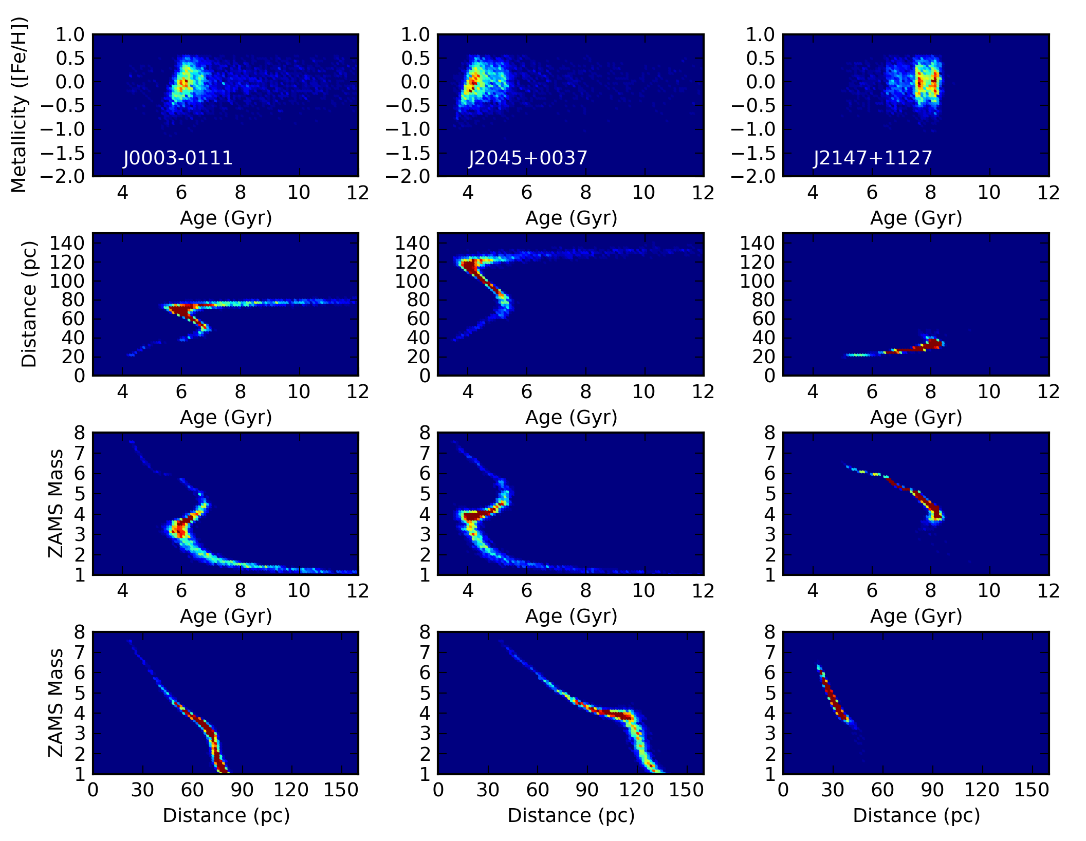
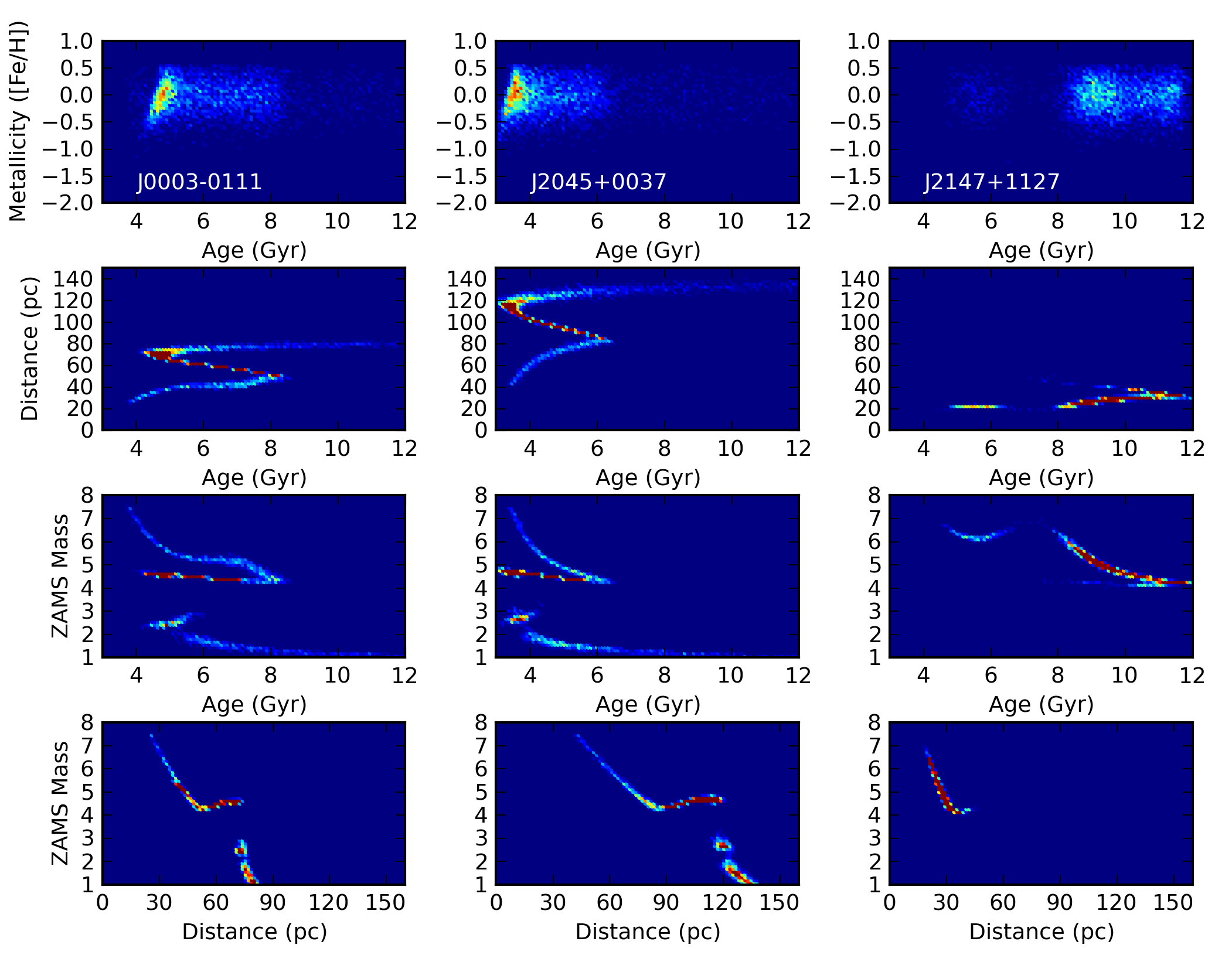
Figure 3 displays the posterior distributions for a single representative star (J0003$-$0111), fit with the Montgomery et al. WD models and each of the four IFMRs we have studied. There are detailed similarities in all four cases, and in fact the contours for all IFMRs peak near 6 Gyrs and 65 pc, yet the distributions are subtly different from one IFMR to another. For instance, the upper distance limits extend $\sim$10 pc further for the Weidemann IFMR and the Salaris et al. Piecewise IFMR than for the other IFMRs and the lower distance extrema move even more substantially. Such comparisons for other stars also show broadly similar results from one IFMR to another and in subsequent analyses we will compare summary statistics for the different IFMRs, rather than the entire posterior distributions.

Figure 3.— Posterior probability projections in the age, distance, ZAMS mass planes for J0003$-$0111 for each of four IFMRs and the Montgomery et al. WD cooling models. These IFMRs, from left to right, are the Williams et al., Weidemann, Salaris et al. Linear, and Salaris et al. Piecewise relations.

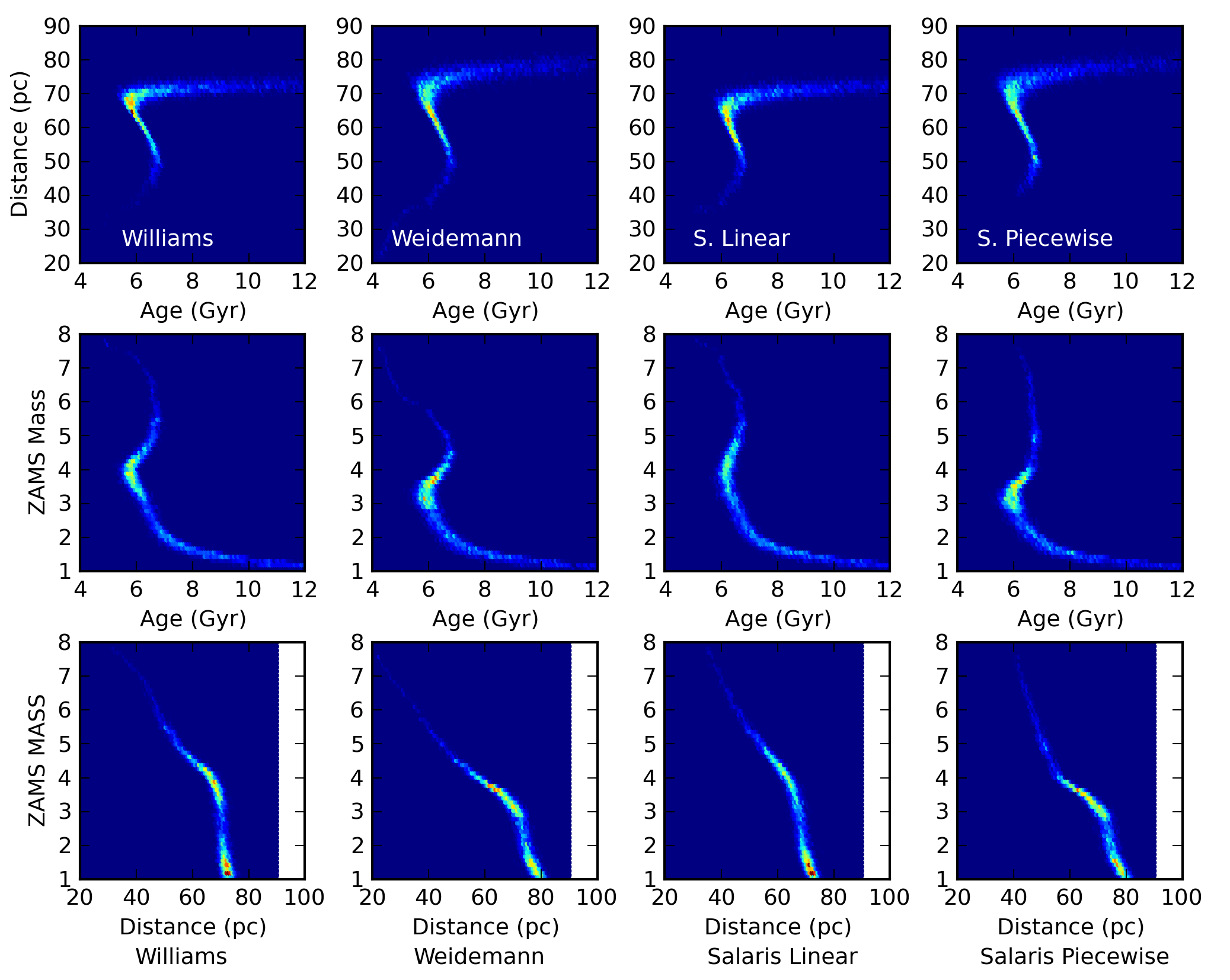
Figure 4 displays the marginal (i.e., collapsed, one dimensional) posterior distributions for the four fitted parameters for the three WDs presented in Figures 1 & 2 for all four IFMRs. The different IFMRs are color coded and the solid and dashed histograms indicate fits based on Montgomery et al. and Renedo et al. WD models. As expected, all of the metallicity distributions for all stars using all IFMRs are the same and in fact are very close to the priors on [Fe/H] (we find posterior values 0.27 $<$ $\sigma$([Fe/H]) $<$ 0.29). The metallicity distributions are truncated at [Fe/H] = +0.5 because that is the upper metallicity limit of the Dotter et al. isochrones. The age distributions are more complicated than the [Fe/H] distributions, yet are broadly consistent among the IFMRs but not always between the two WD models. The distance and ZAMS mass distributions can be different from one IFMR to another. Because distance is a directly measurable quantity, in principle coupling this type of analysis with precision trig parallaxes for the right stars could rule for or against particular IFMRs within some mass ranges. For instance, for both J0003$-$0111 and J2045$+$0037, greater distances are possible with some IFMRs than with others.

Figure 4.— Marginal posterior distributions for the four fitted parameters for each of the three stars presented in Figure 1. All four IFMRs are presented as color-coded histograms with green for Weidemann, blue for Williams et al., cyan for Salaris et al. Linear, and red for Salaris et al. Peicewise Linear. The Montgomery et al. models are indicated with solid lines and the Renedo et al. results are indicated with dashed lines.

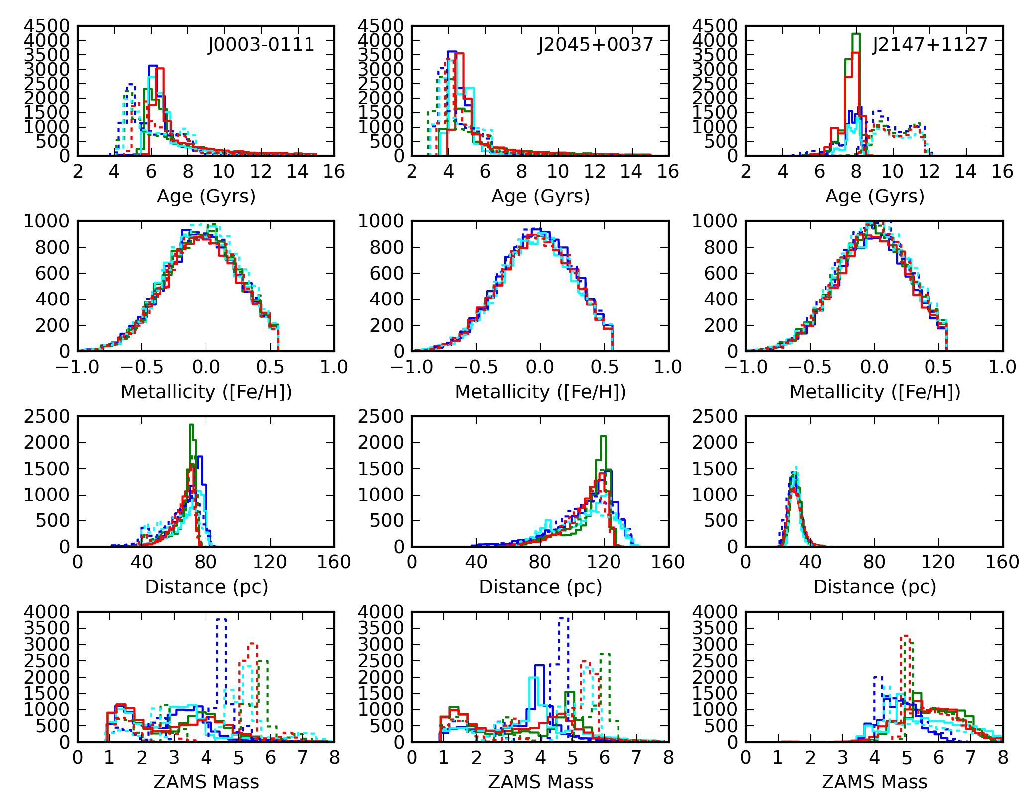
Figure 5 summarizes the age information for all 28 DAs that we have analyzed using all four IFMRs and the Montgomery et al. WD models. The horizontal axes in all panels display age assuming the Williams et al. IFMR and the vertical axes display the age difference under Williams et al. and under the other IFMRs. The points and error bars indicate both the average and median ages along with the 68% confidence intervals. We note that these confidence intervals are not derived to be symmetric about the median or average, but rather mark the values beyond which the last 16% of distribution at each end resides. Despite differences in the shapes of the age distributions, for most of these old DA WDs, both the median and average ages are essentially identical from one IFMR to another. The exception are 3 or 5 of the 8 youngest WDs, and to a lesser extent, 2 WDs near 6.2 Gyr, all of which systematically differ in age between the Williams et al. IFMR on the one hand and the other three IFMRs on the other hand. Overall this is good news given the current state of uncertainty in the IFMR. The average age uncertainty for these 28 DAs analyzed under the Montgomery WD models is $\pm^{10.5\%}_{13.5\%}$.

Figure 5.— Average (black star symbols) and median (red circle symbols) differences in calculated ages for 28 DAs for each of four IFMRs for the Montgomery et al. models. The error bars represent the 68% confidence intervals in the marginalized posterior age distribution for the wider of the two age fits.

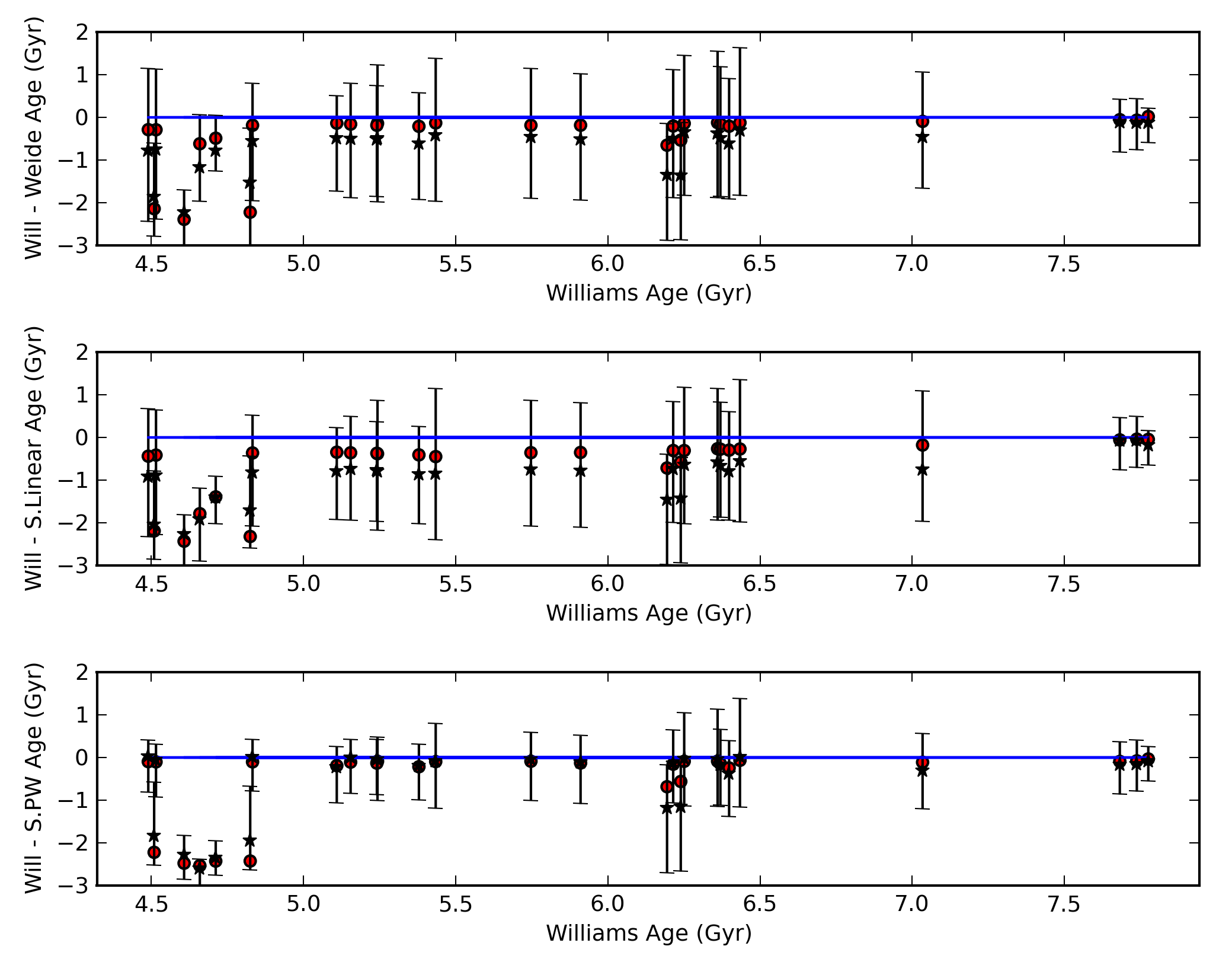
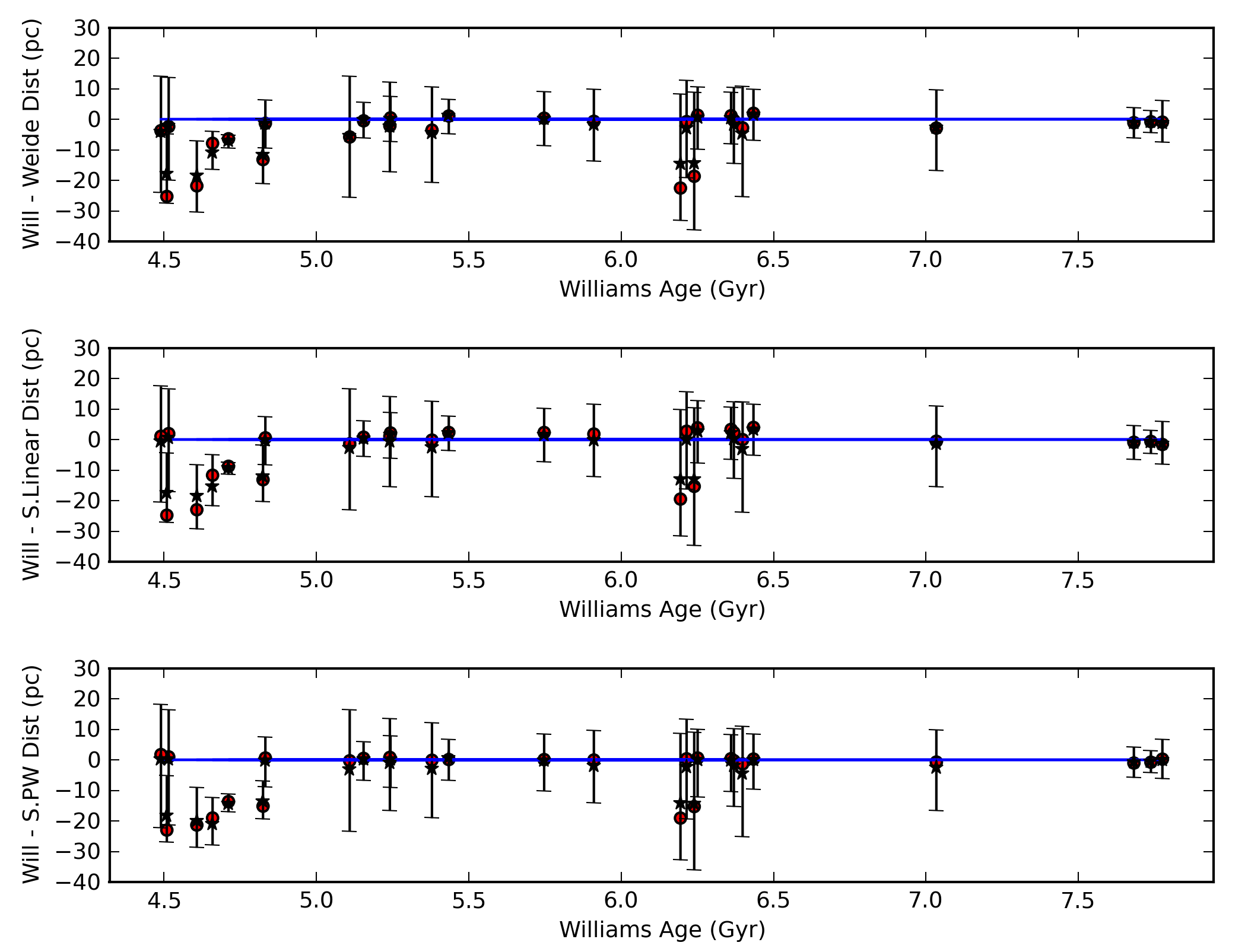
Figure 6 presents the differences in median distances for each of the 28 DAs as analyzed with each of the four IFMRs. As with Figure 5, the error bars represent the 68% confidence interval of the distance posterior distribution for the wider of the two distributions being compared. Most stars have statistically similar median and average distances no matter which IFMR is used, but there are differences among some of the same stars that were inconsistent in Figure 5. This figure reiterates a point from Figure 4, which is that for some stars, follow-up precision distances could rule for or against any particular IFMR within a particular mass range.

Figure 6.— Similar to Figure 5, but now the y-axis displays the difference in distance fits for each of the four IFMRs.

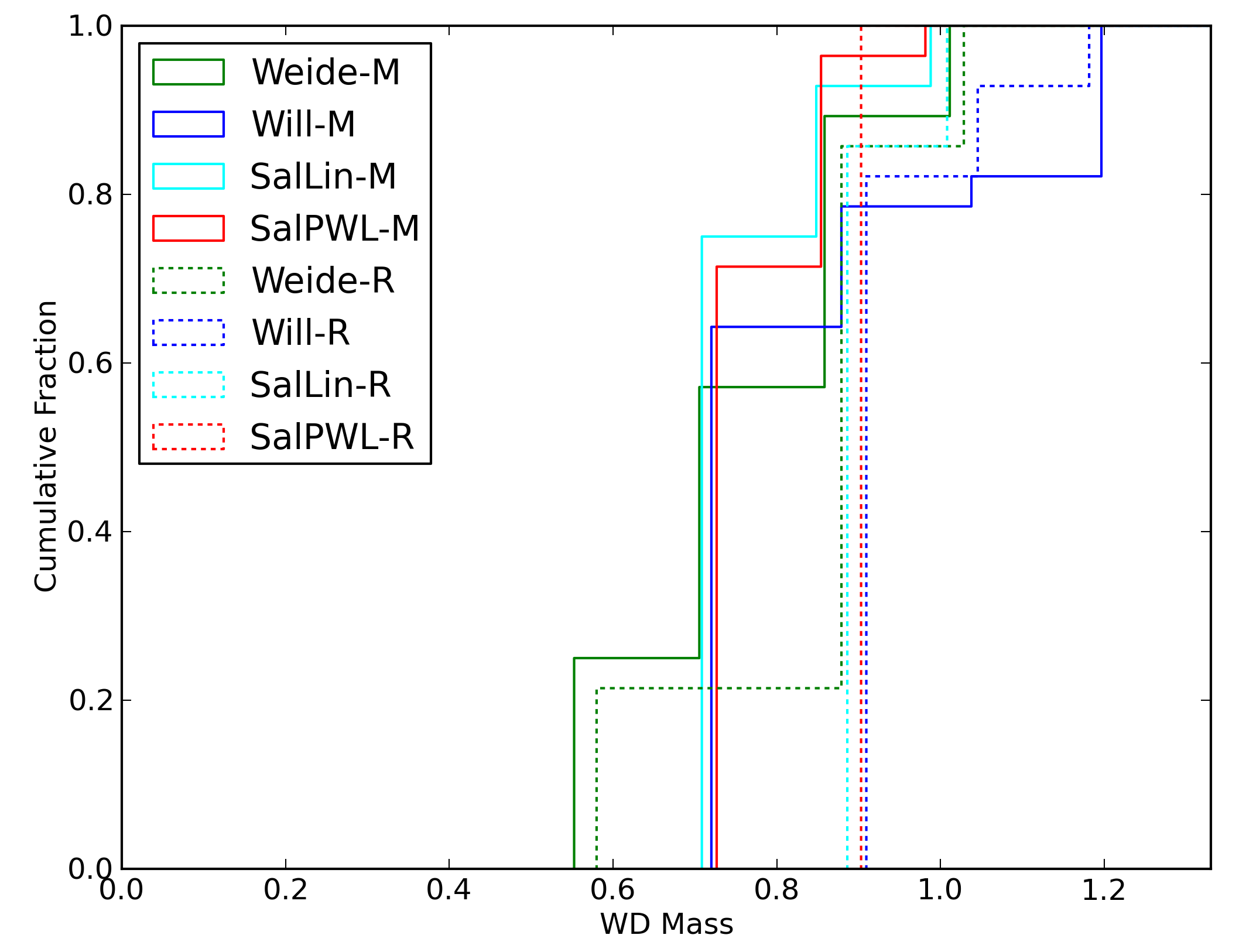
In Figure 7 we present the cumulative distributions of the fitted median WD masses for our 28 DAs under each of the four IFMRs and both WD models. These cumulative distributions are often different from each other, particularly the Williams et al. IFMR versus the other IFMRs, and there is an offset from one WD model to another. In all cases, our sample of 28 DAs likely contains a few high mass WDs. The Williams et al. IFMR fits imply that ten WDs may have masses greater than 0.9 M_⊙ (J074721+24, J0821+3727, J0947+4459, J1102+4030, J1130+1002, J1317+0621, J1534+0711, J1722+2848, J2147+1127, and J2342$-$1001). We remind the reader that these masses are not directly fit and that a constraining prior on distance could decrease any of these implied masses. Yet, because of the relative rarity of high mass WDs and the likely onset of crystallization for stars of this age and implied mass (Metcalfe, Montgomery, & Kanaan 2004), these objects merit additional scrutiny.

Figure 7.— Cumulative distribution of median WD masses for 28 DAs analyzed under four IFMRs. Line styles are the same as in Figure 4.

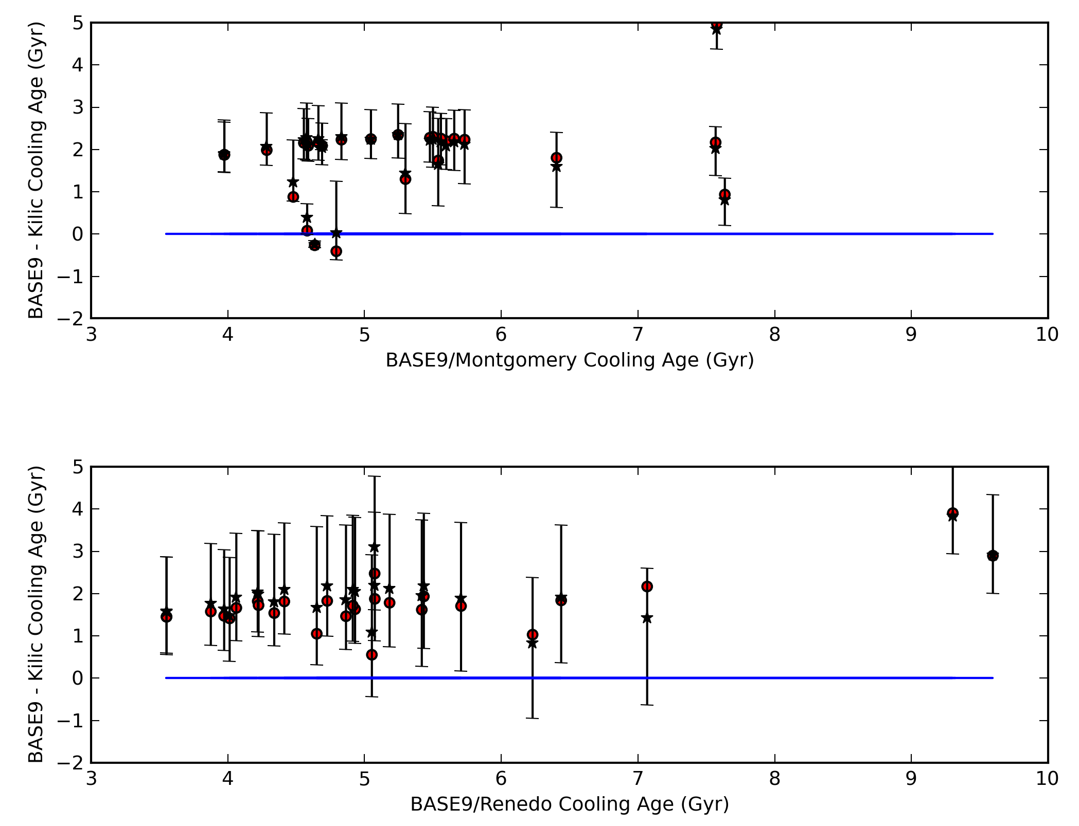
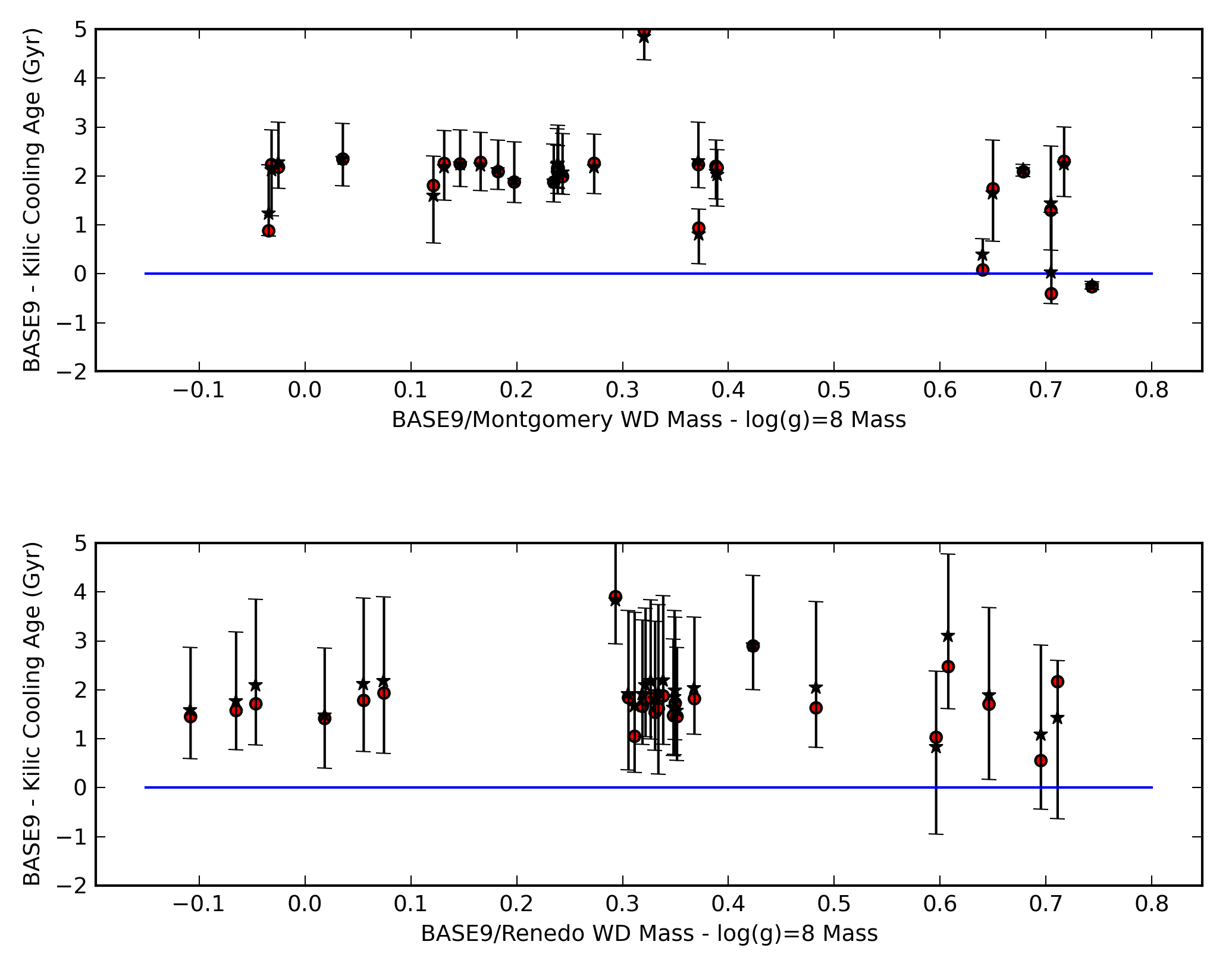
We can make an initial quantitative comparison between the traditional approach to deriving individual WD ages by comparing the ages derived by Kilic et al. (2010) with our Bayesian results for these 28 WDs. Kilic et al. did not have access to spectroscopic log($g$) information, and thus did not have masses for these stars. Instead, they assumed log($g$) = 8.0, which is a common approach in this situation and equivalent to assuming all WDs have masses of $\sim$0.58 M_⊙ for this $T_{eff}$ range (Bergeron et al. 1995). Because WDs have a narrow mass peak near 0.6 M_⊙ (e.g., Liebert, Bergeron, & Holberg 2005 who find a standard deviation around this peak of $<0.2M_{\odot}$), this approach should yield only a slight age bias with some scatter introduced by the actual WD masses. Additionally, Kilic et al. report the WD cooling ages, whereas BASE-9 yields total WD ages. We thus calculated the posterior distribution of cooling ages for each of these 28 WDs in order to compare our results and those of Kilic et al. (2010). Figure 8 displays that comparison with both the Montgomery et al. (top panel) and Renedo et al. (bottom panel) WDs. There is a systematic offset of $\sim$ 1-2 Gyr for most stars broadly distributed across age.

Figure 8.— Average (black star symbols) and median (red circle symbols) differences between the BASE-9 cooling ages and the Kilic et al. cooling ages. The error bars represent the 68% confidence intervals of the BASE-9 cooling age posterior distribution. Kilic et al. did not provide age uncertainties.

If the entire systematic between our ages and the Kilic et al. ages were due to the Kilic et al. assumption that log($g$) = 8, we should see a strong correlation between the difference of our WD mass estimate and the Kilic et al. mass assumption versus the difference in WD cooling ages (BASE-9 cooling age minus Kilic et al. cooling age). We plot that comparison in Figure 9. There is no meaningful correlation in this diagram, so the systematic age difference cannot be primarily due to the log($g$) = 8 assumption. This bolsters the case that the traditional age determination technique can give substantially different answers than our Bayesian approach and thus that the standard, step-wise process for determining ages of individual WDs may yield misleading results.

Figure 9.— The difference between the median BASE-9 WD mass estimates and the log(g)=8 masses versus the difference in WD cooling ages between BASE-9 and those derived by Kilic et al. The symbols and error bars have the same meaning as in Figure 8.

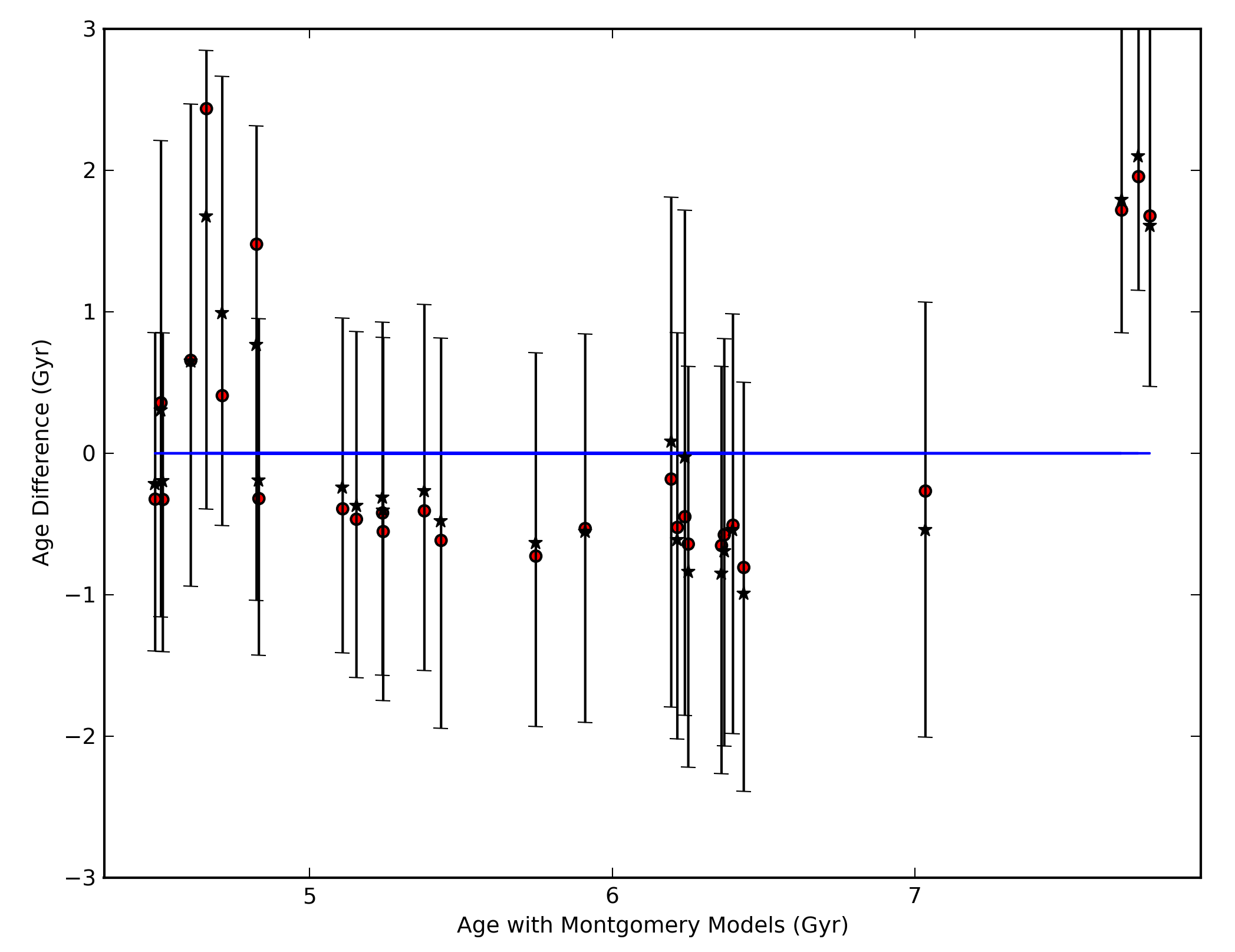
Up until this point, we have noted a few differences among the results based on whether we used Montgomery et al. or Renedo et al. WD models, but we have not directly compared our results based on these two models. In Figure 10 we provide this comparison employing the Williams et al. IFMR. It is comforting to see that these two modern WD cooling models yield consistent results for 25 of these 28 WDs. For the three WDs that are inconsistent, they differ in the sense that the Renedo et al. models imply ages $\sim$2 Gyr older than the Montgomery et al. models. Interestingly, these stars are all cooler than $T_{\rm eff}$ = 5500 based on the Bergeron et al. model atmosphere colors, and it is precisely in this region where theorists expect non-grey atmospheres, as incorporated in the Renedo et al. models, to be important in modelling cool WDs. Unfortunately, we cannot ascribe this difference to grey vs. non-grey atmospheres because 50+% of the posterior mass distributions for all three of these WDs lies beyond the Renedo et al. upper mass limit (0.934 M_⊙), and therefore these fits with the Renedo et al. models required extensive extrapolation in mass.

Figure 10.— Montgomery et al. ages versus Renedo et al. ages. The vertical axis gives the difference in the sense Renedo $-$ Montgomery, with the symbols and errors bars as in Figure 5. These fits were made with the Williams et al. IFMR.

5. Conclusions

We have applied a self-consistent and robust Bayesian statistical approach to determining the ages, distances, and ZAMS masses of individual WDs. We find that age, distance, and ZAMS mass are correlated in complicated posterior distributions. While these correlations make sense in terms of the non-linearities of stellar evolution, they are too complex to be quantified by traditional error propagation methods. Additionally, because the age posterior distributions are often asymmetric, traditional techniques can yield misleading ages.

We find that for our DA sample in the age range of $\sim$4 to 8 Gyrs, that SDSS $griz$ photometry supplemented by quality $JHK$ photometry is sufficient to derive ages with errors $<$ 15%. Furthermore, these ages are often (but not always) insensitive to which of the current modern IFMRs one uses. We expect that these age uncertainties could be substantially reduced with additional information from spectroscopy or parallax measurements that would constrain WD masses.

We also find that distances to some of the WDs in our sample could rule for or against one or more of the IFMRs within particular mass ranges. These distances could be incorporated into a new BASE-9 analysis to derive a new principled estimate of the IFMR. Trigonometric parallaxes for some of these objects would be particularly valuable.

Statistical Method

The statistical methods we use are a special case of those described in Stein et al. (2013), see also DeGennaro et al. (2009) and van Dyk et al. (2009). Because our WDs are nearby and at high Galactic latitude, we fix $A_{\rm V}=0$. The helium abundance, important in the evolution of the WD precursor, is set in the DSED models at $Y=0.245+1.6$Z. We specify the likelihood function for fitting the remaining stellar parameters, $\mbox{\boldmath{$\Theta$}}=$ ($m-M$, [Fe/H], log(IMF), log(age)). Specifically, for a single white dwarf, this likelihood can be written,

$$L(\mbox{\boldmath{$\Theta$}}|\mbox{\boldmath{$X$}},\mbox{\boldmath{$\Sigma$}})={1\over\sqrt{(2\pi)^{n}|\mbox{\boldmath{$\Sigma$}}|}}\exp\left(-{1\over 2}\Big{(}\mbox{\boldmath{$X$}}-\mbox{\boldmath{$G$}}_{\textrm{WD}}(\mbox{\boldmath{$\Theta$}})\Big{)}^{\top}\mbox{\boldmath{$\Sigma$}}^{-1}\Big{(}\mbox{\boldmath{$X$}}-\mbox{\boldmath{$G$}}_{\textrm{WD}}(\mbox{\boldmath{$\Theta$}})\Big{)}\right)$$

where $X$ is the vector of observed photometric magnitudes, $\Sigma$ is the variance-covariance matrix of the observation errors, and $\mbox{\boldmath{$G$}}_{\textrm{WD}}(\mbox{\boldmath{$\Theta$}})$ is the vector of predicted photometric magnitudes as a function of the stellar parameters. $\mbox{\boldmath{$G$}}_{\textrm{WD}}$ takes as input the mass of the WD precursor and the total age of the star, passes that through the DSED stellar evolution models, one of four IFMRs, one of two WD interior models, and a WD atmosphere model to predict the photometric magnitudes.

Our Bayesian analysis is based on the posterior distribution of $\Theta$, namely

$$p(\mbox{\boldmath{$\Theta$}}|\mbox{\boldmath{$X$}},\mbox{\boldmath{$\Sigma$}})\propto L(\mbox{\boldmath{$\Theta$}}|\mbox{\boldmath{$X$}},\mbox{\boldmath{$\Sigma$}})p(\mbox{\boldmath{$\Theta$}}),$$

where $p(\mbox{\boldmath{$\Theta$}})$ is the prior distribution for the stellar parameters. The prior distribution quantifies knowledge about the likely values of the stellar parameters that we have before considering the current data set. The posterior distribution combines this information with that in the data and summarizes all of the available information including the current data. We specify $p(\mbox{\boldmath{$\Theta$}})$ independently for each of the stellar parameters; details appear in Table 1.

Statistical inference for the stellar parameters is based on a Monte Carlo simulation from their posterior distribution. These simulations are plotted to represent the posterior distribution, e.g., in Figures 1-3 or summarized by their mean or median to estimate the parameters. Although the likelihood is based on a simple Gaussian distribution, the dependence of its mean on the stellar parameters can be highly non-linear, potentially leading to an irregular posterior distribution for $\Theta$, see, e.g., Figures 1-3. We use a Markov chain Monte Carlo (MCMC) sampler on the joint posterior distribution of $m-M$, [Fe/H], and log(age), which is obtained by numerically integrating $p(\mbox{\boldmath{$\Theta$}}|\mbox{\boldmath{$X$}},\mbox{\boldmath{$\Sigma$}})$ over the log(IMF). We use a set of initial MCMC iterations to approximate the posterior variance-covariance matrix of $m-M$, [Fe/H], and log(age) and then run a Metropolis sampler that uses this matrix in its jumping rule. We typically thin the sample by a factor of 100-500 to obtain a subsample with lower correlation. We only present results of WDs where the resulting MCMC sampler, after appropriate burn in, appears to deliver a reliable representation of the posterior distribution. We recover the posterior ZAMS mass distribution by sampling it from its conditional posterior distribution after the MCMC run is complete.

We performed a sensitivity analysis on our priors by relaxing the two ($m-M$ and [Fe/H], see Table 1) for which we have no independent data. Our nominal priors were relaxed to $m-M$ = 4 $\pm$ 5 ($63\pm^{568}_{57}$ pc) and [Fe/H] = 0 $\pm$ 1.0. We then reran 7 WDs with the Renedo et al. interior models and the Williams et al. IFMR. For these 7 WDs, although the average metallicities decreased by $\sim$0.4 dex, because our models bound the upper limit of [Fe/H] at $+$0.5, the other parameters differed very little. The average ages differed by 0.040 to 0.167 Gyr, or 0.77% to 3.17%. The average distances differed by only 0.4 to 2.8 pc, and always $\leq$ 3.6%. The average ZAMS masses for these stars differed by 0.07 to 0.18 M_⊙, always $\leq$ 5%.

Table 1Prior Distributions
Quantity	Prior
$m-M$	Gaussian($\mu=4.0$, $\sigma=2.5$), equivalent to dist = $63\pm^{136}_{43}$ pc
Fe/H	Gaussian($\mu=0.0$, $\sigma=0.3$)
IMF	log(IMF) $\sim$ Gaussian($\mu=-1.02$, $\sigma=0.67729$) from Miller & Scalo (1979)
	subject to MWD,up, upper ZAMS mass limit to produce a WD = 8 M⊙
log(age)	Uniform above 250 Myrs, 0 below