Modeling interacting dynamic networks: I. Preferred degree networks and their characteristics
Abstract
We study a simple model of dynamic networks, characterized by a set preferred degree, . Each node with degree attempts to maintain its and will add (cut) a link with probability (). As a starting point, we consider a homogeneous population, where each node has the same , and examine several forms of , inspired by Fermi-Dirac functions. Using Monte Carlo simulations, we find the degree distribution in steady state. In contrast to the well-known Erdős-Rényi network, our degree distribution is not a Poisson distribution; yet its behavior can be understood by an approximate theory. Next, we introduce a second preferred degree network and couple it to the first by establishing a controllable fraction of inter-group links. For this model, we find both understandable and puzzling features. Generalizing the prediction for the homogeneous population, we are able to explain the total degree distributions well, but not the intra- or inter-group degree distributions. When monitoring the total number of inter-group links, , we find very surprising behavior. explores almost the full range between its maximum and minimum allowed values, resulting in a flat steady-state distribution, reminiscent of a simple random walk confined between two walls. Both simulation results and analytic approaches will be discussed.
1 INTRODUCTION
Networks are ubiquitous, emerging in natural structures as well as man-made artifacts. Examples of the former range from the microsopic, e.g., neuron architectures, to the cosmic, e.g., galactic filaments. For the latter, they include critical infrastructures, e.g., power or transportation grids, as well as virtual webs, such as Facebook and LinkedIn. Understanding their characteristics and behaviors is clearly important [1, 2, 3, 4, 5]. In recent years, the statistical properties of complex networks such as their topology [6, 7], their evolution over time [3, 8], and dynamical processes on them [9, 10] have been widely investigated. However, most of these studies have focused on single isolated networks. By contrast, networks in the real world are often intimately intertwined. At the cellular level, drastically different networks, from the cytoskeleton to regulation and signaling, form intricate patterns of interdependence. Similarly, infrastructure networks such as airlines, ground transportation, power grids, and telecommunications are highly interdependent. Meanwhile, the internet plays a critical role by interacting with all of them. In the last few years, the significance of interacting networks is coming onto center-stage, and many scientists and engineers turn their attention to various aspects of such interactions. Examples of these studies include critical infrastructure interdependencies [11, 12, 13, 14], and approaches such as the multilayer method for modeling traffic flows on an underlying infrastructure [15].
Since real interacting networks are extremely complex, even building good models for them is already challenging, not to mention developing reliable analytic approaches. Our goal here is to introduce a model that is sufficiently simple so that analytic solutions are within our reach. Further, in deference to realistic interacting networks, our links will be dynamic. Specifically, our model is motivated by social networks in which the nodes are individuals and the links represent contacts between them. As social connections are made and broken, links are added or cut, resulting in a dynamically evolving network structure. In the long term, the goal is to investigate not only the interactions between such dynamic networks, but also to include the degrees of freedom associated with the nodes, e.g., opionion, wealth, health, etc. [9, 10, 16, 17, 18, 19, 20, 21, 22]. In such models, the network structure and the attributes of the nodes co-evolve, coupled by nontrivial dynamic feedback.
In a series of papers, we present a model of dynamical links which we believe reflects natural and typical human behavior, i.e., a network with preferred degrees. In any society, individuals have their preference for associating with a certain number of friends. We model this preference by a ‘preferred degree’ () for each node. Of course, depends on the ‘personality’ of the individual and varies from person to person. Further, it may change intrinsically with time; perhaps slowly as one ages and the need for contacts changes. may also adapt to varying external circumstances, such as moving to a different neighborhood, joining a workplace or escaping a raging epidemic or a war. Many authors have tried to model such dynamic networks by introducing a ‘rewiring’ of links [9, 10]. While this has the (technical) advantage of keeping the total number of links constant, in some circumstances, it might be more realistic to remove this constraint. For example, in the 2003 SARS epidemic outbreak [23], the Singapore government closed all schools which drastically cut down interactions among children. Obviously, the students did not ‘rewire’ to new contacts in order to replace the classmates lost by this decree. Instead, such a situation can be modeled by a which drops by an order of magnitude (e.g., from 100 classmates to 10 family members). A more detailed discussion of epidemic spreading on preferred degree networks is beyond the scope of this paper but can be found in [16].
In this first paper of a series, we focus exclusively on the dynamics of links, i.e., the number of nodes and their degree remain fixed, and the nodes carry no degrees of freedom. Since interacting networks are complex, we will begin with a ‘baseline study,’ namely, the simplest possible preferred degree network – a homogeneous population – in which all individuals have the same and do not discriminate against, or in favor of, any other individual when adding or cutting links. We will introduce rules on how an individual node decides to add or cut a link and discuss the degree distribution after the system has settled into a stationary state: . Despite the appearance of randomness (with mean degree ), our steady-state degree distribution differs significantly from the Poisson form found in the standard Erdős-Rényi random network [24].
Then, we will introduce two such networks and couple them with arguably the simplest of couplings: When an individual adds or cuts a link, this action is performed on a inter-network link with fixed probability . Such a deceptively simple generalization leads to remarkably rich behaviors, as we extend the characterization to distributions of intra- and inter-network degrees. In particular, we begin with networks which differ by only one of the three parameters, , where is the number of nodes. We find that the total number of crosslinks between the two networks, , plays a key role in characterizing the interactions, while its stationary distribution, , displays highly non-trivial behavior.
This paper is organized as follows: In section , we present the specifications of our model, first for a homogeneous population with a single preferred degree and then a heterogeneous one consisting of two different groups. We also introduce several quantities that serve to characterize the interaction between the two groups, e.g., the distribution of crosslinks. In section , we present the results from Monte Carlo simulations along with an approximate mean field theory which allows us to understand some of the remarkable behaviors. We close with a summary and outlook in section , while deferring some technical details to the Appendices.
2 SPECIFICATIONS OF THE MODELS
Since our goal is the behavior of interacting networks with preferred degrees, we begin with a detailed description of a network with a single preference, namely a homogeneous population. Thereafter, we will describe a simple way to induce interactions between such networks and study their properties. Such interacting networks can be considered as a highly idealized model of a society with inhomogeneous populations.
2.1 Homogeneous populations
Though the notion of a preferred degree network has been introduced previously by the present authors and their collaborators [26, 27, 16, 25] , let us recapitulate the main ingredients here. We consider a network consisting of (static) nodes (with no degrees of freedom) and a dynamically evolving set of links. Each node is endowed with the same fixed attributes: and , the probability that it will create and destroy a link, respectively, given that it has links. For simplicity, we restrict our study to the special case and denote by . Starting from an empty network, we generate links as follows. In each time step (attempt), we select a node at random and find its degree, . Then, with probability , this node creates a new link to a randomly chosen node, which is not already connected to it. Otherwise, this node cuts one of its existing links at random, with probability . Self-loops and multiple connections are not allowed. To model an individual’s natural preference for some finite number of contacts, , we choose a to be close to when , crossing over to when . The simplest with this property is the step function (i.e., for and otherwise), as a good model for a very ‘rigid personality,’ adding or cutting links as soon as the preferred degree is unmet or exceeded. We have also considered more moderate ‘personalities,’ modeled by a Fermi-Dirac function:
| (1) |
where plays the role of an individual’s ‘rigidity.’ Although there are innumerable ways to choose the form of , we restrict our analysis to the form in Eq. (1). Studying the details of is not the primary goal here. Instead, our interest focuses on universal statistical properties of the collective behavior of many individuals, such as the degree distribution, which we denote by .
2.2 Heterogeneous populations with two groups
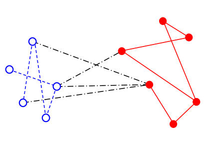
Keeping in mind that our distant goal is the interaction between networks of possibly distinct types, our next step in that direction is modest: the study of two networks of the same type, namely, two preferred degree networks. Needless to say, in a typical heterogeneous society, individuals will have a range of preferences and flexibilities. As a first attempt, we will focus on a population with just two different preferences (), but the same personality (rigid). In particular, we will refer to the first group as ‘introverts,’ since these individuals prefer fewer contacts, while group consists of ‘extroverts.’ We will also allow the groups to have different sizes in general, with nodes, i.e., a total of nodes.
If there is no contact between two such groups, the above forms a complete set of specifications. But, as soon as we wish to model their interactions, many possibilities arise. In this first study, we restrict ourselves to only one mechanism, by introducing a new parameter , the probability that a node interacts with an inter-group node. In an attempt, a random node from the entire population is chosen. Given the chosen node’s degree, , will determine if a link is to be added or cut. Whether adding or cutting, the action will be executed on an inter- or an intra-group link with probability or . In other words, is the chance that the action (adding or cutting) is taken on a crosslink. In general, the two groups can be assigned different values: 2. In a sense, these are associated with how strongly the networks interact, since 2 corresponds to a system consisting of two independent, homogeneous networks. At the other extreme, models a system with crosslinks only. Meanwhile, it is natural to expect the most ‘symmetric’ case, to correspond to a single, homogeneous population. Yet, surprising differences emerge when simulations are carried out.
Given that we are dealing with two networks, a variety of degree distributions can be defined. Specifically, in addition to , the distribution of the total number of contacts associated with a node in group ( in this study), we will study four other degree distributions, namely, the intra- and inter-group degree distributions of each network. Let us introduce the notations in the following. Let and be associated with, respectively, the intra-group and inter-group degrees of a node in group . A specific example is provided in Figure 1, with () specified explicitly in the caption. In this way, for each group, we will study two distributions, and . With this notation, it is clear that generically, . We should emphasize that, though the ‘total degree’ is just the sum (), the distributions , , and contain very different information. For example, in the next section we will demonstrate that and are typically Gaussian-like, while are simple two-tailed exponential distributions.
A more global quantity of interest is , the total number of crosslinks in the system. It is natural to consider its distribution, which we denote by . Of course, there is no a priori reason to expect and the ’s to be related in a simple way. Indeed, we will find that they are generally quite different. Nevertheless, when the system settles in a stationary (steady) state, their averages must obey the equalities
| (2) |
where and is the steady-state distribution, etc. In this paper, we will show that is a rather unusual distribution. In particular, even for populations of , we observe that wanders so slowly that its distribution cannot be reliably measured. Instead, only by restricting ourselves to systems of are we able to find with confidence. In the next section, more details and our findings will be presented.
3 SIMULATION RESULTS AND THEORETICAL CONSIDERATIONS
With the models clearly specified, we can compute all quantities of interest, in principle, and predict the behavior of this system. In practice, the mathematical challenges are insurmountable and, to gain insight into the statistical properties, we perform Monte Carlo simulations on the one hand and on the other, formulate approximation schemes which can capture the main features.
3.1 Statistical properties of a single network
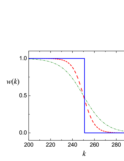
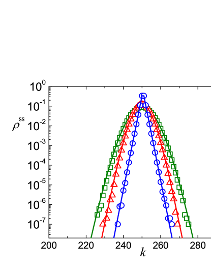
We first establish a baseline for our study, by investigating a homogeneous population. We choose reasonably large () and (), as well as three different ’s (, shown in Fig. 2(a)). To facilitate comparisons between the different cases of , we actually use half integer ’s, e.g., . Starting with an empty network, we follow the stochastic rules above and generate a new configuration with each attempt (at adding/cutting links). Defining a Monte Carlo step (MCS) as updates, we ensure that each node has one chance, on the average, to update its links in a MCS. We discard the first MCS, which appears to be sufficient here for the system to reach steady state. Thereafter, we measure the quantities of interest every MCS and compile averages from measurements (i.e., runs of MCS). Denoting the number of nodes with links in each measurement by , we find through
| (3) |
as illustrated in Fig. 2(b).
For the well known Erdős-Rényi random network, is a Poisson distribution with mean being the average degree. In our network, we clearly expect , and, given that links are created and destroyed at random, we may also expect a Poisson distribution. However, as illustrated in Fig. 2(b), our simulations show otherwise. In the simplest case ( being a step function), is consistent with a two-tailed exponential distribution, (blue circles in Fig. 2(b)). For less rigid populations, depends on the details of for , (green squares and red triangles) but crosses over to the same exponential tails. Our data indicate . In the next few paragraphs, we will present an approximate theory, shown as solid lines in the figure, which provides excellent agreement with this data.
The full description of the stochastic dynamics of our network requires writing down and solving the master equation for the probability of each configuration. Since the mathematical details are quite involved, we present the main results here and leave the technicalities to Appendix A. In particular, we find that the dynamics violates detailed balance so that it is essentially impossible to solve for the exact stationary probability distribution, let alone to compute a quantity like . Thus, finding a reliable approximation scheme is crucial for progress. One possibility is to postulate an equation for directly and compare its predictions with simulation data. Approximating the evolution of by a Markovian birth-death process, we write an expression for :
| (4) | |||
| (5) |
where specifies the rate for a node with degree to change to . Since is non-negative, Eq. (5) is absent for the case. Note that we have cast this expression as the difference of two (probability) currents: Eq. (4) being the net current from to and (5), from to . The advantage of this form is that, in the stationary state, all these currents must vanish, leading to
| (6) |
Thus, once the ’s are given, the stationary can be found explicitly.
Next, we approximate by the following arguments. Focusing on a particular node , we note that the contributions to come from two processes. In one process, node is chosen and a link is cut with probability . In the second process, one of the other nodes, , connected to is chosen and cuts its link to . To account for this rate exactly is quite involved, since there are such nodes, all having varying degrees. Further, once is selected, the probability that it cuts its link to is . Thus, we propose the following rough estimate. We expect that, in a steady state, half of the nodes have “too many” links and, when chosen, will cut. This provides a factor , which we approximate by . Meanwhile, we approximate the various ’s by . The result is that the probability of this second process is simply , so that
| (7) |
A slightly more sophisticated scheme, along with a more carefully detailed argument, can be found in Appendix B. Since the results are not significantly different, especially in cases with moderate ’s, we will continue to rely only on the simple picture here.
A similar argument leads to , so that we obtain
| (8) |
in this approximation. For ‘rigid’ personalities, the solution is trivial,
| (9) |
In other words, this crude scheme predicts , a value remarkably close to the one observed. For more ‘flexible’ individuals, the ’s vary gently around , but cross over to or for or . Thus, the kink in for softens, crossing over to tails governed by the same exponential. For the two cases with finite we simulated, we solve Eq. (8) numerically and show the resultant as solid curves in Fig. 2(b) [16]. Clearly, despite its crudeness, this approximation captures the essense of the steady-state degree distribution.
3.2 Interacting networks with different characteristics
With the statistical properties of a single preferred degree network reasonably well understood, we turn to a system with just two networks and focus on the effects of coupling them in a particular manner (i.e., through described in Section II). Even with this restriction, the varieties of having two networks are limitless. Thus, we further restrict ourselves to studying only ‘rigid’ individuals (), and groups which are identical except for , and, in some cases, . In other words, we attempt to model the interactions between ‘rigid’ introverts and extroverts, albeit in a very simplified fashion. To simulate the model described above, one MCS is defined as updates. Thus, each node is again given one chance, on the average, to take action.
3.2.1 Equal ’s and ’s, but .
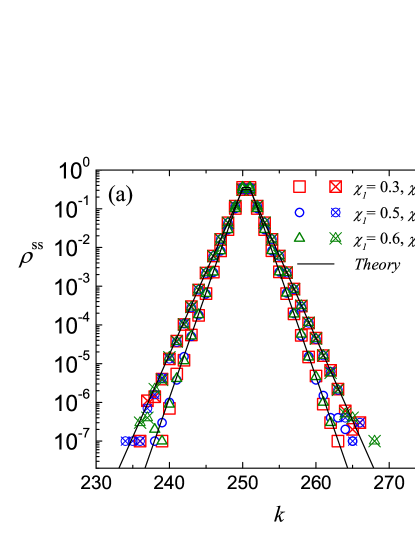
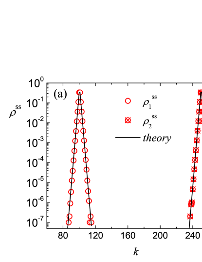
Following our study of the homogeneous population, we begin with two identical groups ( and ) interacting via various ’s. Using a similar scheme – discarding the first MCS and taking measurements separated by MCS, we first consider the total degree distributions in the steady state, . Not surprisingly, these are indistinguishable from the above, namely, exponential distributions. A more interesting scenario appears when the two groups differ only by their ’s, so that . In particular, our simulations show that the are still two-tailed exponentials, but with -dependent tails. Fig. 3(a) illustrates this effect, as we see that results of various ’s collapse into two sets. Intuitively, such a difference can be attributed to ‘frustration’ (in the common psychological sense). If , members of the first group will make frequent attempts to ‘reach out’ to those in the second group. Since this behavior is not reciprocated, we may expect this difference to be manifested in .
Whether we label the observed difference as ‘frustration’ or not, the significant message here is the following. Since the in (7) accounts for the actions by all the other nodes, we must modify it to reflect the different contributions arising from inter- vs intra-group nodes. Thus, when considering a node in, e.g., group , the former contribution is and the latter is . The result of such considerations is the equation
| (10) |
and a similar one for . These lead to
| (11) |
showing that the exponential decay rates deviate from in opposite directions. Remarkably, this simple generalization of the argument advanced above provides a satisfactory explanation, as illustrated by the black lines in Fig. 3(a).
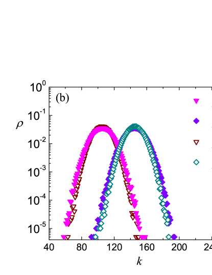
Next, we turn to the separate distributions (also in the steady state, but we suppress the superscript ss for simplicity). Here we encounter several surprises. The first is that these distributions appear to be Gaussians, despite the total being two-tailed exponential! To illustrate this finding, we provide four distributions in Fig. 3(b), for the case . To resolve this quandary, we turn to a better quantity for describing the connectivity associated with a node in a system with two groups, namely, the joint distribution . (There should be no confusion, as we dropped the subscript .) Representing the probability that a node has intra-group links and inter-group links, it is related to the ’s by projections
| (12) | |||||
| (13) |
In the above case, we can describe as a relatively sharp ‘ridge,’ situated along and descending very steeply (exponentially) to the ‘valley floor.’ As we move along this ridge, the variations are more gentle, but as we venture further from the summit, begins to descend as a Gaussian) . Thus, both of the simple projections show the Gaussian profile, while the special projection reveals the exponential distribution.
Examining these Gaussians closer, we see that both ’s have means around , while both ’s are spread around . Further all are typically much broader, , than the two-tailed exponential distributions whose width is . Further, it is remarkable that the and data can be described, very roughly, by the binomial distributions and respectively. This naïve picture comes from partitioning links into crosslinks (average of and , as a rough guess) and intra-group links. We should caution the reader that, despite repeated reference to Gaussians and binomials, these distributions are of course, not precisely so. To study their details, such as skewness and kurtosis, is beyond the scope of this work. Instead, we will discuss a more serious challenge in the next paragraph.
The second discovery is more intriguing, namely, the emergence of two very different time scales. While it takes only MCS for an initially empty network to ‘relax’ into systems with , we find that MCS is sufficient for us to collect good data for . We will refer to this as the short time scale: . During this period, the distributions appear to settle into the Gaussians noted above. However, when examined at much later times (e.g., or MCS), the centers of these Gaussians appear to wander slowly (though their widths are essentially unchanged). In other words, there is a much larger time scale, after which the system finally relaxes into the true steady state. Denoted by , it appears to be much greater than MCS. Such behavior is observed even for the most symmetric case ! We will return to this puzzle later. Here let us turn to other parameter choices for our two interacting networks.
3.2.2 Equal ’s and ’s, but
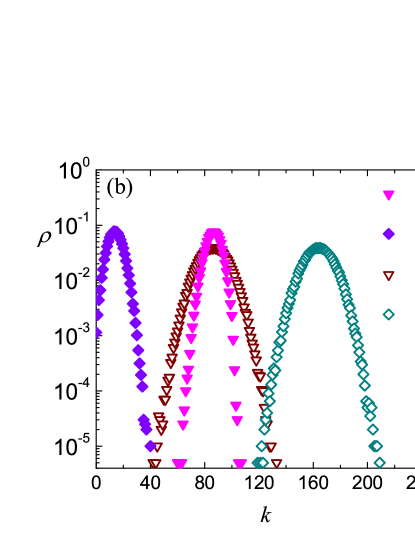
As indicated above, one main motivation for studying two groups is the general perception that there are introverts and extroverts in our society. Thus, we explore a simple initial step: all parameters being equal except the ’s. We expect that such a system should display ‘frustration’ (again, in the psychological sense). The ‘introverts’ are ‘frustrated’ since the ‘extroverts’ reach out to them, generating more links than the introverts prefer; in turn, the extroverts are also dissatisfied by seeing their links constantly cut by the introverts. However, by exploring systems with only moderate differences, specifically, and , we detect no conspicuous signs of such frustration. Indeed, we find no new surprises here. Illustrated in Fig. 4 are degree distributions (obtained from short runs, ) for the case with and . In Fig. 4(a), we see the familiar two-tailed exponential distributions for the total degree distributions – with means at the two different ’s and tails of . The remaining distributions, shown in Fig. 4(b), are also similar to the above, i.e., being essentially Gaussians. The most prominent feature here is that their means and widths appear quite disparate. Of course, we must have since both equal the average total number of crosslinks in the systems. If we use the ad hoc scheme above – declaring the average crosslinks for each node to be , we arrive at . The complements are intra-group links, i.e., and here. As can be seen in the figure, these values are roughly acceptable. The binomials, depicted above, give similarly rough portraits of these ’s. The main challenge, as described earlier, remains to be the understanding of the slow wandering of these ’s at much longer time scales.
3.2.3 Equal ’s and ’s, but .
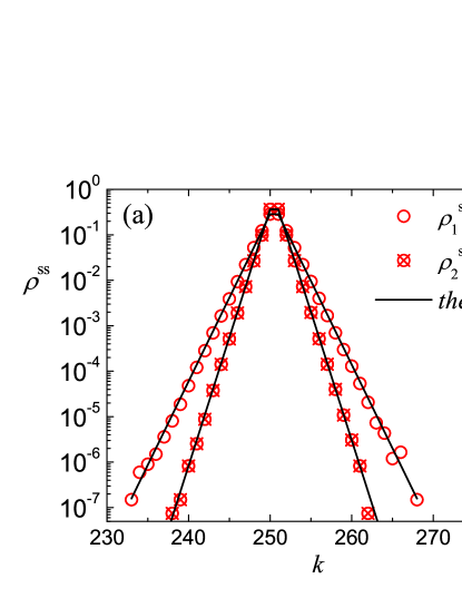
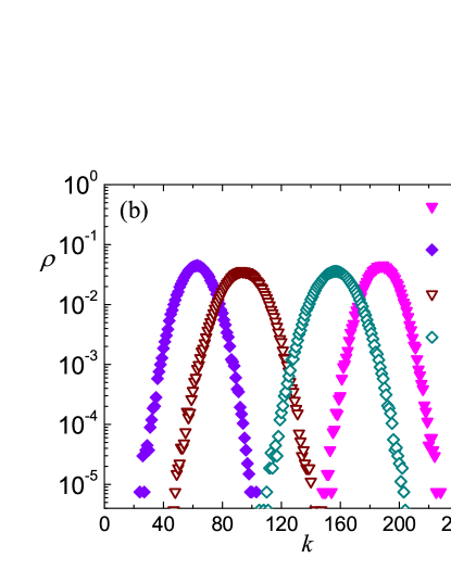
To complete the skeletal picture, let us report some findings of systems with unequal group sizes. In particular, we simulated a system with (), again for short periods of time (). The various degree distributions are shown in Fig. 5. Not surprisingly, the totals have settled into two-tailed exponential distributions, though with different ’s. Since the ’s are the same, the simple argument leading to Eq. (10) is modified only by the different number of nodes in each group. Specifically, if we again focus on a node in group , then the (adding/cutting) actions of the inter-group nodes would be enhanced by a factor of . If the ’s were also different, then the in Eq. (7) would become
| (14) |
In case , this factor becomes , so that we can use
| (15) |
to predict approximate distributions (black lines in Fig. 5(a)). Again, we find very good agreement with the data here.
Meanwhile, for the separate distributions , we again observe Gaussians, though the but the means are now located at four distinct values. As above, it is possible to provide rough estimates for these results. Since , we are not surprised that peaks at , a value twice that for , . Arguably, we may regard these mean degrees as the result of an effective , i.e., , giving us . If we further impose an ad hoc assumption – namely, that the average of these ’s should not change – then we arrive at and . Remarkably, such rough arguments differ only about from the simulation results. While this approach cannot be taken as a good understanding of the phenomena observed, it may provide a stepping stone towards a more reliable theory.
3.3 Statistical properties of the total number of crosslinks, .
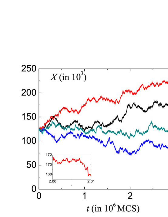
Though degree distributions are standard quantities for characterizing networks, we have seen that, in a system with just two groups, additional challenges arise when we consider distributions of different types of links. The puzzles uncovered can be traced to, we believe, a single characteristic of such systems, namely, , the total number of links between the two groups. In particular, the slow wanderings of the means in can be related to the slowly varying , while at shorter time scales, is well described by a random distribution of among the nodes. This subsection is devoted to a few initial steps towards the understanding of the behavior of .
To connect with the results from the last subsection and to emphasize the challenge we face, we show the data associated with an apparently symmetric system: , , . These parameters are chosen to be comparable to those studied in the previous subsections. In Fig. 6, four runs of over MCS are not inconsistent with the traces of random walkers. Note that, in all cases, (we start with empty networks) and at early times, , a number consistent with the simple estimate . Thereafter, wanders widely. Of course, this random walk is bounded, by from below and ( here) from above. The latter is an estimate, assuming that every node has all of its connections as crosslinks. From the figure, we see that these runs have not yet reached these boundaries. In other words, it would take MCS for this system to finally settle in the true steady state. Meanwhile, as the inset shows, is relatively constant within any interval of MCS, while the fast mixing of crosslinks between the nodes allows an individual to relax into an approximate Gaussian. Indeed, given , these quasi-stationary distributions fit quite well to another binomial, namely, .
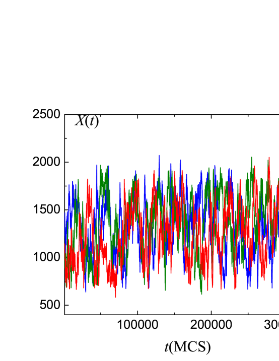
The next natural step is to probe deeper into the hypothesis that is indeed an unbiased random walk, between some ‘soft walls’ and . But, to reach steady state after say, MCS, we must consider much smaller systems (along with smaller ’s). For example, with a system an order of magnitude smaller, and , we expect a random walk to traverse the full range of in about steps. Since a step in will occur in just a few attempts, a good estimate of the traversal time is MCS. Thus, we can expect the system to settle over runs of MCS. When Monte Carlo simulations are carried out (using the most symmetric case: ), these expectations are indeed borne out. In Fig. 7, we display three short sections (each MCS long), obtained from partitioning a single long run ( MCS). Note that indeed traverses the full range in each case.
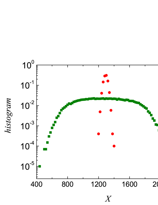
With confidence that the system has reached steady state, we compile a histogram, , from this trace and show the result (olive squares) in Fig. 8. Note that this distribution is relatively flat, around the mean of approximately (i.e., ) with soft cutoffs at both ends. Such a wide and fairly flat ‘plateau’ in is consistent with the idea that executes a simple random walk between two soft walls, located approximately at and .
In the next paper, we will provide other measures which strengthen our hypothesis. Here, let us end with addressing a natural question: Is there any difference between our ‘most symmetric’ case () and a single homogeneous network of nodes with ? In particular, what can be expected if we arbitrarily label half of the latter nodes as ‘red’ and the rest ‘blue,’ and compile a histogram for the total number of red-blue links in the system? Simulations show a remarkably different picture. Illustrated with solid red circles in Fig. 8 this distribution is much sharper than and well described by a Gaussian, with mean close to and standard deviation . The value of the mean is not surprising, especially if we recall that, in our simulations, the effective is . As for , it is precisely the value of the most naïve expectation, from applying the central limit theorem to adding random variables distributed according to . It is remarkable how two models which appear to be so similar exhibit such drastically different behavior. In particular, by modeling interactions between two identical groups with a single parameter, , we encounter counter-intuitive phenomena.
4 SUMMARY AND OUTLOOK
In this paper, we introduced the idea of a stochastically evolving network with preferred degrees. The key feature of our models is that each node can add or cut one of its links, depending on whether it finds itself with too few or too many (compared to some built-in ‘preferred’ number of) contacts. To establish a baseline, we focus first on a single homogeneous isolated network, in which every node ‘prefers’ degree . Specifically, when chosen, a node (with degree ) will create or destroy a link with probability . For simplicity, we only studied models with , while modeling how ‘intolerant’ an individual is, when it finds , by the expression (1). We showed that even in such simple models, the dynamics violates detailed balance, so that the long-time limit is a non-equilibrium steady state. With generally unknown probability distributions and non-trivial probability currents, an exact and analytic approach is all but impossible. Instead, we explore the statistical properties by Monte Carlo simulations and a variety of mean-field approaches. Simulating mainly the most rigid () population, we discovered that an initially empty network of nodes (with ) settles into a steady state quite quickly ( MCS). The degree distribution is a double exponential, around : . A simple mean-field argument, in the context of an approximate master equation, leads to , which agrees well with data. For more flexible populations, is Gaussian-like around and, for large , crosses over to the exponentials above. Our mean-field theory can be generalized appropriately and provides similarly good agreement with the simulation results. Of course, the system will not display this type of behavior for extreme values of , and (e.g., near zero) and we believe the theory will break down in those limits. Nevertheless, for generic points in parameter space, we are confident that the main features of this adaptive network are not difficult to understand, both intuitively and quantitatively.
We then introduced a second preferred degree network and coupled it to the first, through , the probability that a node adds or cuts a crosslink (between the networks). With two networks, the parameter space is already so large that a completely systematic study is beyond our scope. We focused on three cases where the two networks differ by only one of the three parameters (). Seemingly a simple extension of the homogeneous case, this model provides a rather wide range of interesting results, from the mundane and comprehensible to the surprising and puzzling. The total degree distribution of each network is not seriously affected by the interaction and can be reasonably well explained by extending the approximation scheme for the single network case. By contrast, serious challenges emerge when we consider the more detailed distributions: and , associated with intra- and inter-group degrees, and , respectively. Though both total ’s remain two-tailed exponentials, all these new distributions are roughly Gaussians, with means and widths that are yet to be clearly understood. More importantly, we studied a global quantity which is suitable for characterizing the inter-network interactions, namely, the total number of crosslinks in the system, . Remarkably, it displays a very slow dynamics, as well as extensive fluctuations. For example, even after MCS, all of our runs for (in the ‘most symmetric’ case of ) exhibit what appears to be an unbounded, unbiased random walk! By lowering the system parameters to and running up to MCS, we finally observed a stationary distribution for . Being almost flat and broad, this is also not well understood yet.
These initial findings provide us with first steps in this study of interacting networks. The next steps will be presented in the next three papers of this series. Let us provide a preview of the rest of the series. In a second paper, we will present a more systematic study of the statistical properties of as a function of the parameters of the two preferred degree networks: , . Since the underlying dynamics does not obey detailed balance, an explicit expression for the the microscopic stationary distribution through equilibrium statistical mechanics is not possible. As a result, we rely mostly on Monte Carlo simulations. A certain level of theoretical understanding can be obtained from various approximation schemes for a master equation governing the evolution of . In the third paper, we will consider an extreme limit: and . We coin the name ‘XIE’ model for this case of ex̱treme i̱ntroverts and e̱xtroverts, in which every introvert prefers zero contacts (and only cuts links) and every extrovert prefers as many friends as possible (and always adds links). This limit is interesting for several reasons. The only relevant parameters left are and . Meanwhile, detailed balance is restored in this limit and so, an explicit microscopic stationary distribution of the system can be obtained. Nevertheless, cannot be computed analytically, though a mean field approach seems to be quite adequate for predicting its key features. Most surprisingly, there is an extraordinary transition in the system (), as the ratio is varied through unity [25]. Further, using a self-consistent mean field approximation, we are able to predict (with no fit parameters!) , except for the case . In the last paper, we will present results for models involving several other forms of interaction. Perhaps more realistic, these will include letting an individual have two ’s, to differentiate actions taken with inter- and intra-network contacts. Clearly, our primary focus for this series rests on the statistical properties of systems in steady states. The full time-dependent behavior of dynamic networks, clearly much richer and more complex, will be considered in the future.
We conclude with a few comments on how to extend our model to more realistic cases. First, there is typically a full spectrum of ‘preferences’ in every society, and so one should really consider a set, . Second, in our model here, every individual can connect with every other one, which clearly fails to capture the more complex structures of a real society, from simple spatial proximities to social status and subtle ethnic divides, etc. Third, we should explore more realistic models of real phenomena, where nodes (individuals) are endowed with dynamic degrees of freedom, e.g., opinions, wealth, or health. These degrees of freedom in turn determine the connections (links) between individuals in a society, leading to a fully co-evolving model of node and link dynamics.
Beyond social networks, a worthy goal would be the understanding of the interactions between dramatically different networks, such as those listed in the Introduction. Clearly, achieving such a goal would have significant and long-term impact on both network science and the welfare of our species.
Appendix A Stochastic dynamics of a single network: Exact master equation and violation of detailed balance
A single network can be described by an adjacency matrix (symmetric in our case, as the links are undirected), where the elements indicate the absence (presence) of the link between nodes and . Since self-loops are not allowed, for all . A complete analytical description of the stochastic evolution of our model is provided by , which is the probability of finding configuration at time , given an initial configuration . Since our focus is on a dynamics without memory, i.e., a Markov process, we can write down the discrete master equation for as follows. The change over one attempt, is
| (16) |
where is the rate for configuration to change to . Note that, since each has elements, the configuration space in which evolves consists of the vertices of a unit cube in -dimensional space. In this setting, each attempt is seen to be just a step from one vertex to another along an edge of this cube.
Explicitly, consists of a sum over terms, each corresponding to an attempt at changing the state of a link. We begin with the probability to choose a particular node, : . Next, we need its degree, , which is obtained by summing up all elements along, say, the row : . From here, we attempt to add a link with probability , or cut with probability . Consider first a cutting action, which can occur for one of the existing links, so that the total probability for, say, to change from to (by node ) is Meanwhile, none of the other links changes in this attempt. Thus, the term describing this action is
| (17) |
where
| (18) |
A similar term can be written to describe the adding action. All together, we have
| (19) |
Once the rates are known explicitly, we can check if they satisfy detailed balance or not. The Kolmogorov criterion [28] states that a set of ’s satisfies detailed balance if and only if the product of ’s around any closed loop in configuation space is equal to that around the reversed loop. In our case, all loops can be regarded as sums over “elementary closed loops,” i.e., ones which goes around a plaquette (or face) on our -cube. Thus, we only need to focus on such elementary loops. Clearly, such a loop involves two links, e.g., by adding two links from a given , followed by cutting them to return to the original . As a specific example, suppose we start with an which has neither an link nor an one. Then the sequence
| (20) |
denotes adding these two and cutting them, while the rest of is left unchanged. Apart from an overall factor of , the product of the ’s associated with this loop is
| (21) |
Now, the reversed loop can be denoted as
| (22) |
associated with the product
| (23) |
Of course, we can find the difference explicitly and verify that it does not vanish in general. To appreciate this fact more easily, note that, e.g., the factor appears in (21) but not in (23). From these considerations, we conclude that detailed balance is violated here.
We should re-emphasize the following. In our case, the products of ’s around many elementary loops are the same as those of the reversed loops (e.g., two links involving 4 different vertices). However, detailed balance is satisfied only if all loops are ‘reversible.’ So, showing just one ‘failed loop’ is sufficient for us to conclude that detailed balance is violated, the consequences of which are quite serious (see, e.g., [29] for further details.).
Appendix B Approximation schemes for the transition rates,
We provide the simple arguments used for the transitions rates appearing in Eqns. (6). These lead to slightly more sophisticated versions of the expressions (7,8,10,15) in the main text.
First, we consider the single network case and argue as follows to obtain a simple expression for , the probability that a node with degree will lose one of its links. We focus on a particular node () with degree . In each attempt, the probability for the node itself to be chosen is just and then for it to cut a link is . In addition, node can lose a link if one of the other nodes connected to it (say node ) chooses to cut a link, and to cut the link to node (i.e., the link here). Now, the probability is for one of these nodes to be chosen. Assuming all nodes are equally likely to have too many or too few links, we approximate the probability for cutting to be . Finally, if were chosen, then the probability it cuts the link is , which we replace by , by invoking a mean-field approximation. Combining these factors, the chance that node will lose a link due to the action of others is . Thus, we have
| (24) |
A further approximation assumes and we arrive at (7). Clearly, a similar argument leads to the probability for adding links, , yielding a slightly different version of (8). In the specific cases we studied, these two versions are so similar that both predictions are consistent with the simulation data. If were , then we can expect more discernable differences. Investigations along such lines remain to be undertaken.
Turning to systems with two populations, let us first consider those with equal ’s and ’s but . Let us focus on a node in group , so that the probability for it to be chosen is and for it to cut is again . The new aspect here is that there are two groups of nodes which may be connected to , corresponding to a total of links. Each of these has some probability that it will cut its link to . The chance of choosing from the (intra-group) nodes is . As before, we assume that is the probability such a node () will cut. Now, the novel feature is that with probability it will cut an intra-group link while is the chance it will cut the link. If we make the further approximation (since both are in group ), then these considerations lead to . A similar argument for the actions of a node in group leads to , so that we have
| (25) |
Combining a similar argument for , we arrive at (10). A pattern for such considerations begins to emerge, so that expressions such as (14) and (10) can be easily derived.
However, we should point out that it is much more unreliable to develop arguments like these for the case of , which is the reason for using ad hoc schemes such as “average of and .”
References
References
- [1] Strogatz S H 2001 Nature 410 268
- [2] Albert R and Barabási A-L 2002 Rev. Mod. Phys. 74 47
- [3] Dorogovtsev S N and Mendes J F F 2002 Adv. Phys. 51 1079
- [4] Newman M E J 2003 SIAM Rev. 45 167
- [5] Estrada E, Fox M, Higham D and Oppo G-L (eds) 2010 Network Science: Complexity in Nature and Technology (Springer, New York)
- [6] Watts D J and Strogatz S H 1998 Nature (London) 393 440
- [7] Albert R, Jeong H and Barabási A-L 1999 Nature (London) 401 130
- [8] Barabási A-L and Albert R 1999 Science 286 509
- [9] Gross T and Blasius B 2008 J. R. Soc. Interface 5 259
- [10] Barrat A, Barthelemy M and Vespignani A 2008 Dynamical processes on complex networks (Cambridge University Press)
- [11] Rinaldi S, Peerenboom J and Kelly T 2001 IEEE Contr. Syst. Mag. 21 11
- [12] Panzieri S and Setola R 2008 Int. J. Model. Ident. Contr. 3 69
- [13] Buldyrev S V, Parshani R, Paul G, Stanley H E and Havlin S 2010 Nature (London) 464 1025
- [14] Buldyrev S V, Shere N W and Cwilich G A 2011 Phys. Rev. E 83 016112
- [15] Kurant M and Thiran P 2006 Phys. Rev. Lett. 96 138701
- [16] Jolad S, Liu W, Schmittmann B and Zia R K P 2012 PLoS ONE 7(11) e48686
- [17] Zanette D H and Risau-Gusmán S 2008 Journal of biological physics 34 135
- [18] Gross T, and Kevrekidis I G 2008 EPL 82 38004
- [19] Shaw L B and Schwartz I B 2008 Phys. Rev. E 77 066101
- [20] Schwarzkopf Y, Rákos A and Mukamel D 2010 Phys. Rev. E 82 036112
- [21] Marceau V, Noël P A, Hébert-Dufresne L, Allard A and Dubé L J 2010 Phys. Rev. E 82 036116
- [22] Wang B, Cao L, Suzuki H and Aihara K 2011 Journal of Physics A: Mathematical and Theoretical 44 035101
- [23] http://www.moe.gov.sg/media/press/2003/pr20030326.htm
- [24] Erdős P and Rényi A 1959 Pub. Math. 6 290
- [25] Liu W, Schmittmann B and Zia R K P 2012 EPL 100 66007
- [26] Platini T and Zia R K P 2010 J. Stat. Mech. Theory Exp. 2010 P10018
- [27] Zia R K P, Liu W, Jolad S and Schmittmann B 2011 Physics Procedia 15 102
- [28] Kolmogorov A N 1936 Math Ann. 112 155
- [29] Zia R K P and Schmittmann B 2007 J. Stat. Mech. Theory Exp. 2007 P07012