Non-Abelian off-diagonal geometric phases in nano-engineered four-qubit systems

Abstract

The concept of off-diagonal geometric phase (GP) has been introduced in order to recover interference information about the geometry of quantal evolution where the standard GPs are not well-defined. In this Letter, we propose a physical setting for realizing non-Abelian off-diagonal GPs. The proposed non-Abelian off-diagonal GPs can be implemented in a cyclic chain of four qubits with controllable nearest-neighbor interactions. Our proposal seems to be within reach in various nano-engineered systems and therefore opens up for first experimental test of the non-Abelian off-diagonal GP.

1 Introduction

When a state of a quantal system evolves in time, it may pick up a geometric phase (GP) factor that reflects the geometry of the underlying state space. This phase factor turns out to be undefined if the end-points of the path correspond to distinguishable, i.e., orthogonal, states. This fact led Manini and Pistolesi [1] to introduce off-diagonal GPs that capture interference information related to state space geometry in cases where the standard GP is not defined. This off-diagonal GP was subsequently verified experimentally for neutron spin [2, 3] and its mixed state counterpart was identified in Refs. [4, 5, 6].

Kult et al. [7] generalized the off-diagonal GP in Ref. [1] to the non-Abelian case. A non-Abelian GP is a unitary matrix that reflects the geometry of a Grassmann manifold, i.e., a space of subspaces of some given dimension of a complex vector space [8]. Each subspace along a path in a Grassmann manifold may represent the post-measurement state of an incomplete projective measurements [9, 10] or an encoding of a quantum computational system [11, 12]. The non-Abelian setting offers the additional possibility of partially overlapping subspaces giving rise to a richer off-diagonal GP structure than in the Abelian case.

Here, we provide an explicit physical setting for the non-Abelian off-diagonal GPs in terms of a cyclic chain of four qubits with nearest-neighbor interaction. The setup can be used for realizations of non-Abelian off-diagonal GPs in different kinds of nano-engineered systems, such as in quantum dots [13], atoms in optical lattices [14], and topological insulators [15]. Our proposal seems to be within reach with current technology and therefore opens up for first experimental test of the non-Abelian off-diagonal GP.

2 Non-Abelian off-diagonal GPs

We first briefly review the basic theory of non-Abelian off-diagonal GPs. Suppose $\mathcal{H}$ is the system’s Hilbert space and consider the smoothly parametrized decomposition

$$\mathcal{H}=\mathcal{H}_{1}(s)\oplus\cdots\oplus\mathcal{H}_{\eta}(s),\ s\in[0,t]$$ (1)

into $\eta$ mutually orthogonal subspaces. We assume that $\dim\mathcal{H}_{l}(s)=n_{l}$ are constant for the duration of the evolution and $\sum_{l=1}^{\eta}n_{l}=\dim\mathcal{H}\equiv N$. The evolution $s\mapsto\mathcal{H}_{l}(s)$ is a path $\mathcal{C}_{l}$ in the Grassmann manifold $\mathcal{G}(N;n_{l})$, i.e., the space of $n_{l}$-dimensional subspaces of the $N$-dimensional Hilbert space $\mathcal{H}$.

Let $\mathcal{F}_{l}(s)=\{l^{p}(s)\}_{p=1}^{n_{l}}$ be a smoothly parametrized frame (ordered orthonormal basis) spanning the subspace $\mathcal{H}_{l}(s)$. Define the quantities

$$\sigma_{kl}=\left[\mathcal{F}_{k}(0)|\mathcal{F}_{l}(t)\right]{\bf T}e^{\int_{0}^{t}A_{l}(s)ds},$$ (2)

where $\left[\mathcal{F}_{k}(0)|\mathcal{F}_{l}(t)\right]_{pq}=\langle k^{p}(0)|l^{q}(t)\rangle$ is the $n_{k}\times n_{l}$ overlap matrix of the frames $\mathcal{F}_{k}(0)$ and $\mathcal{F}_{l}(t)$ and $[A_{l}(s)]_{pq}=\langle\partial_{s}l^{p}(s)|l^{q}(s)\rangle$ is the Wilczek-Zee connection [16] along the path $\mathcal{C}_{l}$.

In the case where $k=l$, the quantity

$$U_{g}^{(1)}(\mathcal{C}_{l})=\Phi[\sigma_{ll}]=\left(\sqrt{\sigma_{ll}\sigma_{ll}^{\dagger}}\right)^{\ominus}\sigma_{ll},$$ (3)

$\ominus$ being the Moore-Penrose pseudoinverse [17, 18] obtained by inverting all nonzero eigenvalues, is the standard open path non-Abelian GP [19, 20]. If $\sigma_{ll}$ is full rank, $\Phi[\sigma_{ll}]$ is a unitary $n_{l}\times n_{l}$ matrix; if the rank is nonzero and lower than $n_{l}$, the non-Abelian GP is partially defined [20] corresponding to the case where the subspaces at the end-points of the path $\mathcal{C}_{l}$ in the Grassmann manifold $\mathcal{G}(N;n_{l})$ are partially overlapping, i.e., their nonzero overlap matrix is not full rank. Note that a partially defined $U_{g}^{(1)}(\mathcal{C}_{l})$ is a partial isometry, i.e., an operator such that $U_{g}^{(1)}(\mathcal{C}_{l})U_{g}^{(1)\dagger}(\mathcal{C}_{l})$ and $U_{g}^{(1)\dagger}(\mathcal{C}_{l})U_{g}^{(1)}(\mathcal{C}_{l})$ are projectors onto the two end-points [20]. In the case of orthogonal subspaces at the end-points of the path $\mathcal{C}_{l}$, $\sigma_{ll}$ vanishes and the non-Abelian GP is undefined. The points along the evolution, where the GP is undefined or partially defined, are considered as singular points of the evolution.

For a set $\{l_{1},\ldots,l_{\kappa}\}$ of distinct indices, each $\sigma_{kl}$, $k,l\in\{l_{1},\ldots,l_{\kappa}\}$, transforms as $\sigma_{kl}\rightarrow U_{k}^{\dagger}(0)\sigma_{kl}U_{l}(0)$, where the two unitaries $U_{k}^{\dagger}(0)$ and $U_{l}^{\dagger}(0)$ induce change of frames of the two subspaces $\mathcal{H}_{k}(0)$ and $\mathcal{H}_{l}(0)$. Thus, $\sigma_{kl}$ transforms non-covariantly since $U_{k}(0)$ and $U_{l}(0)$ can be chosen independently. This transformation property suggests

$$\gamma_{l_{1}\ldots l_{\kappa}}=\sigma_{l_{1}l_{\kappa}}\sigma_{l_{\kappa}l_{\kappa-1}}\cdots\sigma_{l_{2}l_{1}}$$ (4)

as gauge covariant quantities in terms of which the non-Abelian off-diagonal GPs of order $\kappa$ are defined to be

$$U_{g}^{(\kappa)}(\mathcal{C}_{l_{1}},\ldots,\mathcal{C}_{l_{\kappa}}) = \Phi\left[\gamma_{l_{1}\ldots l_{\kappa}}\right]$$ (5)

$$= \left(\sqrt{\gamma_{l_{1}\ldots l_{\kappa}}\gamma_{l_{1}\ldots l_{\kappa}}^{\dagger}}\right)^{\ominus}\gamma_{l_{1}\ldots l_{\kappa}}.$$

Note that $U_{g}^{(\kappa)}(\mathcal{C}_{l_{1}},\ldots,\mathcal{C}_{l_{\kappa}})$ is a property of the ordered set of paths $\{\mathcal{C}_{l_{1}},\ldots,\mathcal{C}_{l_{\kappa}}\}$ in the set of Grassmann manifolds $\{\mathcal{G}(N;n_{1}),\ldots\mathcal{G}(N,n_{\kappa})\}$. The GP in Eq. (3) is contained as the special case where $\kappa=1$.

Similar to the $\kappa=1$ GPs discussed above, the phase factor $U_{g}^{(\kappa)}(\mathcal{C}_{l_{1}},\ldots,\mathcal{C}_{l_{\kappa}})$ is undefined or partially defined if $\gamma_{l_{1}\ldots l_{\kappa}}$ vanishes or is not of full rank, respectively. These points are the singular points of the evolution of the system related to the off-diagonal GPs of order $\kappa$. It has been shown in Ref. [7] that there is no singular point where all the different order non-Abelian GPs are undefined simultaneously.

3 Realization of non-Abelian off-diagonal GPs in a four-qubit system

Our four-qubit system is described by the Hamiltonian

$$\widetilde{H}=F(s)\sum_{k=1}^{4}\left(J_{k,k+1}R_{k,k+1}^{\textrm{XY}}+D_{k,k+1}^{z}R_{k,k+1}^{\textrm{DM}}\right),$$ (6)

where $R_{k,k+1}^{\textrm{XY}}=\frac{1}{2}\left(\sigma_{x}^{k}\sigma_{x}^{k+1}+\sigma_{y}^{k}\sigma_{y}^{k+1}\right)$ and $R_{k,k+1}^{\textrm{DM}}=\frac{1}{2}\left(\sigma_{x}^{k}\sigma_{y}^{k+1}-\sigma_{y}^{k}\sigma_{x}^{k+1}\right)$ are XY and Dzialochinski-Moriya (DM) terms with coupling strengths $J_{k,k+1}$ and $D_{k,k+1}^{z}$, respectively; $\sigma_{x}^{k}$ and $\sigma_{y}^{k}$ being standard Pauli operators acting on qubit $k$. $F(s)$ turns on and off all qubit interactions simultaneously. The cyclic nature of the qubit chain is reflected in the boundary conditions $J_{4,5}R_{4,5}^{\textrm{XY}}=J_{4,1}R_{4,1}^{\textrm{XY}}$ and $D_{4,5}^{z}R_{4,5}^{\textrm{DM}}=D_{4,1}^{z}R_{4,1}^{\textrm{DM}}$.

The Hamiltonian in Eq. (6) preserves the single-excitation subspace

$$\mathcal{H}_{\text{eff}}=\textrm{Span}\{|1000\rangle,|0010\rangle,|0100\rangle,|0001\rangle\}$$ (7)

of the four qubits. In the ordered orthonormal basis $\{|1000\rangle,|0010\rangle,|0100\rangle,|0001\rangle\}$, the Hamiltonian takes the form

$$H=F(s)\left(\begin{array}[]{rr}0&T\\ T^{\dagger}&0\end{array}\right),$$ (10)

were

$$T=\left(\begin{array}[]{rr}J_{12}-iD_{12}^{z}&J_{41}+iD_{41}^{z}\\ J_{23}+iD_{23}^{z}&J_{34}-iD_{34}^{z}\end{array}\right)=USV^{\dagger}.$$ (13)

Here, $U,V$, and $S$ are the unitary and diagonal positive parts in the singular-value decomposition of $T$. We assume $S>0$.

The Hamiltonian in Eq. (10) may be implemented in different physical systems. First, it may describe a cyclic chain of four coupled quantum dots, where the single excitation is encoded in the localized electron spins with double occupancy of each dot being prevented by strong Hubbard-repulsion terms [13]. Secondly, a square optical lattice of two-level atoms with synthetic spin-orbit coupling localized at each lattice site allows for the desired combination of XY and DM interactions, by suitable parameter choices [14]. A third possible realization is provided by the Ruderman-Kittel-Kasuya-Yosida interaction in three-dimensional topological insulators, which may be used to obtain the XY and DM interaction terms in $\widetilde{H}$ [15].

The Hamiltonian in Eq. (10) splits the effective state space into two orthogonal subspaces, i.e.,

$$\mathcal{H}_{\text{eff}}=\mathcal{H}_{1}\oplus\mathcal{H}_{2},$$ (14)

where the subspaces $\mathcal{H}_{1}$ and $\mathcal{H}_{2}$ are spanned by frames $\{|1000\rangle,|0010\rangle\}$ and $\{|0100\rangle,|0001\rangle\}$ respectively. This implies that the time evolution operator on the effective Hilbert space given in Eq. 7 splits into $2\times 2$ blocks according to [13]

$$\mathcal{U}(t,0)=\left(\begin{array}[]{cc}U\cos\left(a_{t}S\right)U^{\dagger}&-iU\sin\left(a_{t}S\right)V^{\dagger}\\ -iV\sin\left(a_{t}S\right)U^{\dagger}&V\cos\left(a_{t}S\right)V^{\dagger}\end{array}\right),$$ (17)

where $a_{t}=\int_{0}^{t}F(s)ds$ is the ‘pulse area’.

Considering paths $\mathcal{C}_{1}$ and $\mathcal{C}_{2}$ traversed by the two subspaces $\mathcal{H}_{1}$ and $\mathcal{H}_{2}$ under $\mathcal{U}(t,0)$, one may notice that these evolutions are purely geometric since the Hamiltonian vanishes along each of them separately. Thus, the four $2\times 2$ blocks of the time evolution operator $\mathcal{U}(t,0)$ contains explicit information about the pair of paths $\mathcal{C}_{1}$ and $\mathcal{C}_{2}$ in the Grassmann manifold $\mathcal{G}(4;2)$ that can be fully captured by the non-Abelian off-diagonal GPs for $\kappa=1$ and $2$. In fact, we find

$$\mathcal{U}(t,0)=\left(\begin{array}[]{cc}\sigma_{11}&\sigma_{12}\\ \sigma_{21}&\sigma_{22}\end{array}\right),$$ (20)

from which we obtain

$$\sigma_{11} = U\cos\left(a_{t}S\right)U^{\dagger},\ \sigma_{22}=V\cos\left(a_{t}S\right)V^{\dagger},$$

$$\gamma_{12} = \sigma_{12}\sigma_{21}=-U\sin^{2}\left(a_{t}S\right)U^{\dagger},$$

$$\gamma_{21} = \sigma_{21}\sigma_{12}=-V\sin^{2}\left(a_{t}S\right)V^{\dagger}.$$ (21)

The $\kappa=1$ and $\kappa=2$ GPs can be found from these quantities as follows.

By assuming that $\cos\left(a_{t}S\right)$ is full rank, we obtain the $\kappa=1$ GPs

$$U_{g}^{(1)}(\mathcal{C}_{1}) = U\left|\cos\left(a_{t}S\right)\right|^{-1}\cos\left(a_{t}S\right)U^{\dagger}$$

$$= (-1)^{c}UZ^{d}U^{\dagger},$$

$$U_{g}^{(1)}(\mathcal{C}_{2}) = V\left|\cos\left(a_{t}S\right)\right|^{-1}\cos\left(a_{t}S\right)V^{\dagger}$$ (22)

$$= (-1)^{c}VZ^{d}V^{\dagger},$$

where $c,d=0,1$ and $Z=\text{diag}\left\{1,-1\right\}$. These GPs are characterized by different sectors whose boundaries are given by pulse area values $a_{t}$ such that one or both eigenvalues of $\cos\left(a_{t}S\right)$ vanish. These points are singular points of the time evolution of the system, where the $\kappa=1$ GPs are undefined or partially defined. Explicitly, when passing through a point where only one of the eigenvalues of $\cos\left(a_{t}S\right)$ vanishes, $d$ changes by one unit and the GPs switch abruptly as $(-1)^{c^{\prime}}\hat{1}\leftrightarrow(-1)^{c}UZU^{\dagger}$ and $(-1)^{c^{\prime}}\hat{1}\leftrightarrow(-1)^{c}VZV^{\dagger}$, where $\hat{1}$ is the $2\times 2$ identity matrix and $c,c^{\prime}=0,1$. If both eigenvalues pass through zero simultaneously, only $c$ changes by one unit corresponding to an overall change of sign. Thus, in this case, the GPs switch abruptly as $UZ^{d}U^{\dagger}\leftrightarrow-UZ^{d}U^{\dagger}$ and $VZ^{d}V^{\dagger}\leftrightarrow-VZ^{d}V^{\dagger}$.

To compute the off-diagonal $\kappa=2$ GPs, we first note that $\sin^{2}\left(a_{t}S\right)\geq 0$. Thus, in the case where both eigenvalues of $\sin\left(a_{t}S\right)$ are non-vanishing, we find the $\kappa=2$ GPs

$$U_{g}^{(2)}(\mathcal{C}_{1},\mathcal{C}_{2})=U_{g}^{(2)}(\mathcal{C}_{2},\mathcal{C}_{1})=-\hat{1}.$$ (23)

If one or both eigenvalues of $\sin\left(a_{t}S\right)$ vanish then the $\kappa=2$ GPs are partially defined or undefined, respectively; these cases correspond to the $\kappa=2$ singular points of the time evolution of the system. However, there is no abrupt switching associated with passage through any of these points since the $\kappa=2$ GPs can only take the value $-\hat{1}$ when it is fully defined. Note that the $\kappa=1$ and $\kappa=2$ singular points are mutually exclusive since they are respectively associated with vanishing eigenvalues of $\cos\left(a_{t}S\right)$ and $\sin\left(a_{t}S\right)$. This confirms the result of Ref. [7] that there are no points where all non-Abelian GPs are undefined.

The independence of the details of the paths $\mathcal{C}_{1}$ and $\mathcal{C}_{2}$ in the $\kappa=2$ GPs is analogous to the single-qubit case, where the corresponding Abelian off-diagonal GP factors always take the value $-1$ except for cyclic evolution where it is undefined [1, 2, 3]. However, in contrast, the non-Abelian case admits a richer off-diagonal GP structure due to the fact that different parallel transporting pulses do in general not commute. To see this, consider a pair of pulses where the first one is characterized by $\widetilde{T}=\widetilde{U}\widetilde{S}\widetilde{V}^{\dagger}$ such that $\sin\left(a_{\tilde{t}}\widetilde{S}\right)=Z$ or $\hat{1}$ (to assure parallel transport also during the second pulse), followed by an arbitrarily long second pulse characterized by $T=USV^{\dagger}\neq\widetilde{T}$. We may write the resulting time evolution operator after the second pulse as

$$\mathcal{U}(t,0) = \mathcal{U}(t,\tilde{t})\mathcal{U}(\tilde{t},0)$$ (26)

$$= \left(\begin{array}[]{cc}\sigma_{12}\widetilde{\sigma}_{21}&\sigma_{11}\widetilde{\sigma}_{12}\\ \sigma_{22}\widetilde{\sigma}_{21}&\sigma_{21}\widetilde{\sigma}_{12}\end{array}\right),$$

where $\sigma_{kl}$ are defined by $T$ and $a_{t}=\int_{\tilde{t}}^{t}F(s)ds$, while $\widetilde{\sigma}_{kl}$ are defined by $\widetilde{T}$ and $a_{\tilde{t}}=\int_{0}^{\tilde{t}}F(s)ds$.

Thus, we obtain the $\kappa=2$ GPs

$$U_{g}^{(2)}(\mathcal{C}_{1},\mathcal{C}_{2}) = \left|\sigma_{11}\widetilde{\sigma}_{12}\sigma_{22}\widetilde{\sigma}_{21}\right|^{\ominus}\sigma_{11}\widetilde{\sigma}_{12}\sigma_{22}\widetilde{\sigma}_{21},$$

$$U_{g}^{(2)}(\mathcal{C}_{2},\mathcal{C}_{1}) = \left|\sigma_{22}\widetilde{\sigma}_{21}\sigma_{11}\widetilde{\sigma}_{12}\right|^{\ominus}\sigma_{22}\widetilde{\sigma}_{21}\sigma_{11}\widetilde{\sigma}_{12}.$$ (27)

In the full rank case, $U_{g}^{(2)}(\mathcal{C}_{1},\mathcal{C}_{2})$ and $U_{g}^{(2)}(\mathcal{C}_{2},\mathcal{C}_{1})$ are unitaries different from $-\hat{1}$. In fact, if we consider pulses, where $\widetilde{\sigma}_{12}$ and $\widetilde{\sigma}_{21}$ commute with $\sigma_{11}$ and $\sigma_{22}$, then we find

$$U_{g}^{(2)}(\mathcal{C}_{1},\mathcal{C}_{2}) = -\left|\sigma_{11}\sigma_{22}\right|^{-1}\sigma_{11}\sigma_{22},$$

$$U_{g}^{(2)}(\mathcal{C}_{2},\mathcal{C}_{1}) = -\left|\sigma_{22}\sigma_{11}\right|^{-1}\sigma_{22}\sigma_{11},$$ (28)

where we have used $\widetilde{\sigma}_{21}\widetilde{\sigma}_{12}=\widetilde{\sigma}_{12}\widetilde{\sigma}_{21}=-\hat{1}$. Therefore, from Eqs. (28) and (21) it follows that the off-diagonal phases $U_{g}^{(2)}(\mathcal{C}_{1},\mathcal{C}_{2})$ and $U_{g}^{(2)}(\mathcal{C}_{2},\mathcal{C}_{1})$ could be any arbitrary SU(2) matrices for appropriate choices of $T$ and $\widetilde{T}$. For instance, the above conditions leading to Eq. (28) can be met by a first pulse characterized by $\widetilde{T}=\lambda\hat{1}$ and $a_{\tilde{t}}=\frac{(2m-1)\pi}{2\lambda}$, $\lambda$ and $m$ being a real positive number and an integer, respectively; followed by a second pulse characterized by arbitrary $T$ and $a_{t}$ such that $\cos\left(a_{t}S\right)$ is full rank.

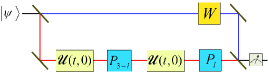
Figure 1: Interferometric setting to measure the non-Abelian off-diagonal GP ($\kappa=2$). The red and blue lines of the interferometer correspond to ancilla qubit states $|0_{a}\rangle$ and $|1_{a}\rangle$, respectively. An input state $|0_{a}\rangle|\psi\rangle$ with $|\psi\rangle\in\mathcal{H}_{l},\ l=1,2$, enters into interferometer and splits into two equal-weighted state vectors each labeled by the ancilla basis states, i.e., $\frac{1}{\sqrt{2}}(|0_{a}\rangle+|1_{a}\rangle)|\psi\rangle$. This is achived by applying a Hadamard transformation to the input state of the ancilla qubit. Thereafter, the state attached to $|0_{a}\rangle$ undergoes successively the transformations $\mathcal{U}(t,0)$, $P_{3-l}$, and $\mathcal{U}(t,0)$, while $|1_{a}\rangle|\psi\rangle$ is left untouched. This is followed by performing the conditional transformation $|0_{a}\rangle\langle 0_{a}|\otimes P_{l}+|1_{a}\rangle\langle 1_{a}|\otimes W$. Next, the two state branches are brought back to interfere by a second Hadamard transformation. Finally, the probability $p$ of finding the final state at the output $|0_{a}\rangle$ branch is measured. By varying the unitary $W$, maximum probability is obtain when $W=\Phi[\gamma_{l(3-l)}]=U_{g}^{(2)}(\mathcal{C}_{l},\mathcal{C}_{3-l})$.

To test the non-Abelian off-diagonal GP ($\kappa=2$), we add an ancilla qubit $\textrm{Span}\{|0_{a}\rangle,|1_{a}\rangle\}$ to the system, prepare the initial state in the superposition $\frac{1}{\sqrt{2}}\left(|0_{a}\rangle+|1_{a}\rangle\right)|\psi\rangle$, and perform conditional unitary dynamics

$$\frac{1}{\sqrt{2}}\left(|0_{a}\rangle+|1_{a}\rangle\right)|\psi\rangle\rightarrow\frac{1}{\sqrt{2}}\left(|0_{a}\rangle\mathcal{U}(t,0)|\psi\rangle+|1_{a}\rangle|\psi\rangle\right)$$ (29)

with $|\psi\rangle$ belonging to $\mathcal{H}_{l},\ l=1,2$. This transformation is followed by the operation $|0_{a}\rangle\langle 0_{a}|\otimes P_{3-l}+|1_{a}\rangle\langle 1_{a}|\otimes\hat{1}_{a}$, the conditional unitary above, and a operation $|0_{a}\rangle\langle 0_{a}|\otimes P_{l}+|1_{a}\rangle\langle 1_{a}|\otimes W$, where $P_{l}$ are projectors onto $\mathcal{H}_{l}$ and $W$ is a variable unitary onto $\mathcal{H}_{l}$. Finally, the ancilla states are transformed by a Hadamard, where $|0_{a}\rangle\rightarrow\frac{1}{\sqrt{2}}\left(|0_{a}\rangle+|1_{a}\rangle\right)$ and $|1_{a}\rangle\rightarrow\frac{1}{\sqrt{2}}\left(|0_{a}\rangle-|1_{a}\rangle\right)$. The resulting total state reads

$$|\textrm{out}\rangle = \frac{1}{2}|0_{a}\rangle\left(P_{l}\mathcal{U}(t,0)P_{3-l}\mathcal{U}(t,0)+W\right)|\psi\rangle$$ (30)

$$+\frac{1}{2}|1_{a}\rangle\left(P_{l}\mathcal{U}(t,0)P_{3-l}\mathcal{U}(t,0)-W\right)|\psi\rangle$$

from which we read off the probability

$$p = \parallel|\textrm{out}\rangle\parallel^{2}=\frac{1}{4}+\frac{1}{4}\langle\psi|\gamma_{l(3-l)}\gamma_{l(3-l)}^{\dagger}|\psi\rangle$$ (31)

$$+\frac{1}{2}\textrm{Re}\langle\psi|W^{\dagger}\gamma_{l(3-l)}|\psi\rangle$$

to detect the system in the state labeled by $|0_{a}\rangle$. By varying $W$ maximum probability is obtain when $W=\Phi[\gamma_{l(3-l)}]=U_{g}^{(2)}(\mathcal{C}_{l},\mathcal{C}_{3-l})$. Thus, the off-diagonal GP can be measured by finding the maximum probability in the output of the interferometer depicted in Fig. 1.

Alternatively, $U_{g}^{(2)}(\mathcal{C}_{l},\mathcal{C}_{3-l})$ can be measured by realizing the interferometer loop directly on the input state $|\psi\rangle\in\mathcal{H}_{l}$ without adding the ancilla qubit. This results in the output state $W^{\dagger}P_{l}\mathcal{U}(t,0)P_{3-l}\mathcal{U}(t,0)|\psi\rangle=W^{\dagger}\gamma_{l(3-l)}|\psi\rangle$, which implies that the probability $\widetilde{p}$ to find the system in $|\psi\rangle$ satisfies

$$\widetilde{p} = \left|\langle\psi|W^{\dagger}\gamma_{l(3-l)}|\psi\rangle\right|^{2}$$ (32)

$$\leq \left|\langle\psi|\left(\sqrt{\gamma_{l(3-l)}\gamma_{l(3-l)}^{\dagger}}\right)^{\ominus}|\psi\rangle\right|^{2}$$

with equality when $W=\Phi[\gamma_{l(3-l)}]=U_{g}^{(2)}(\mathcal{C}_{l},\mathcal{C}_{3-l})$ up to an overall U(1) phase factor. In this way, the non-Abelian SU(2) part of $U_{g}^{(2)}(\mathcal{C}_{l},\mathcal{C}_{3-l})$ can be measured by varying $W$ until maximum is reached.

We demonstrate how the latter setting can be implemented in the four-dot system mentioned above. As demonstrated in [13], a cyclic chain of coupled quantum dots at half-filling can be designed so that it is described by an effective spin Hamiltonian with XY and DM terms resulting from an interplay between electron-electron repulsion and spin-orbit interaction. With $|\!\!\uparrow\rangle,|\!\!\downarrow\rangle$ being the local $s_{z}$-spin basis of each electron, the four-dimensional subspace $|\!\!\downarrow\uparrow\uparrow\uparrow\rangle,\ldots,|\!\!\uparrow\uparrow\uparrow\downarrow\rangle$ is the invariant subspace $\mathcal{H}_{\text{eff}}$ in which the spin Hamiltonian takes the form of Eq. (10) and where the XY and DM coupling strengths can be manipulated separately with time-dependent gate voltages.

Now, to prepare an approriate initial state in the four-dot system, we start by polarizing the spins along the $z$ direction by an external magnetic field. A single spin flip is induced by applying a local magnetic field at one of the sites [21]. Suppose, e.g., we apply it to the first site leading to the spin state $|\psi\rangle=|\!\!\downarrow\uparrow\uparrow\uparrow\rangle\in\mathcal{H}_{1}=\{|\!\!\downarrow\uparrow\uparrow\uparrow\rangle,|\!\!\uparrow\uparrow\downarrow\uparrow\rangle\}$ of the four electrons. In this way, a measurement of $U(\mathcal{C}_{1},\mathcal{C}_{2})$ can be performed by applying sequentially $\mathcal{U}(t,0)$, $P_{2}=|\!\!\uparrow\downarrow\uparrow\uparrow\rangle\langle\uparrow\downarrow\uparrow\uparrow\!\!|+|\!\!\uparrow\uparrow\uparrow\downarrow\rangle\langle\uparrow\uparrow\uparrow\downarrow\!\!|$, $\mathcal{U}(t,0)$, and $P_{1}=|\!\!\downarrow\uparrow\uparrow\uparrow\rangle\langle\downarrow\uparrow\uparrow\uparrow~{}\!\!|+|\!\!\uparrow\uparrow\downarrow\uparrow\rangle\langle\uparrow\uparrow\downarrow\uparrow\!\!|$, where $\mathcal{U}(t,0)=e^{-ia_{t}H}$, followed by the unitary $W^{\dagger}=e^{ib_{t^{\prime}}h}$. The final unitary should be block diagonal with respect to the two orthogonal spin subspaces $\mathcal{H}_{1}$ and $\mathcal{H}_{2}$, which is achieved by implementing

$$h = f(s)\sum_{k=1}^{2}\left(J_{k,k+2}R_{k,k+2}^{\textrm{XY}}+D_{k,k+2}^{z}R_{k,k+2}^{\textrm{DM}}\right)$$ (33)

$$+E(Z_{1}+Z_{2}).$$

Here, $b_{t^{\prime}}=\int_{0}^{t^{\prime}}f(s)ds$ is the ‘pulse area’ and $E(Z_{1}+Z_{2})$ with $Z_{1}=|\!\!\downarrow\uparrow\uparrow\uparrow\rangle\langle\downarrow\uparrow\uparrow\uparrow\!\!|-|\!\!\uparrow\uparrow\downarrow\uparrow\rangle\langle\uparrow\uparrow\downarrow\uparrow\!\!|$ and $Z_{2}=|\!\!\uparrow\downarrow\uparrow\uparrow\rangle\langle\uparrow\downarrow\uparrow\uparrow\!\!|-|\!\!\uparrow\uparrow\uparrow\downarrow\rangle\langle\uparrow\uparrow\uparrow\downarrow\!\!|$ corresponds to a local energy shift of the first and second sites relative the third and fourth site (for instance by applying an inhomogeneous magnetic field over the four-dot system). In the single spin flip subspace, $h={\textrm{diag}}\{T^{\prime},T^{\prime\prime}\}$ with the $2\times 2$ blocks

$$T^{\prime} = \left(\begin{array}[]{cc}E&J_{13}+iD_{13}^{z}\\ J_{13}-iD_{13}^{z}&-E\end{array}\right),$$ (36)

$$T^{\prime\prime} = \left(\begin{array}[]{cc}E&J_{24}+iD_{24}^{z}\\ J_{24}-iD_{24}^{z}&-E\end{array}\right).$$ (39)

The variable unitary $W^{\dagger}$ is generated by $h$ and takes the desired block-diagonal form $W^{\dagger}={\textrm{diag}}\{e^{ib_{t^{\prime}}T^{\prime}},e^{ib_{t^{\prime}}T^{\prime\prime}}\}$ with $e^{ib_{t^{\prime}}T^{\prime}}$ and $e^{ib_{t^{\prime}}T^{\prime\prime}}$ being arbitrary SU(2) operators parametrized by $J_{k,k+1},D_{k,k+1}$, and $E$. Thus, with inital state $|\psi\rangle\in\mathcal{H}_{1}$, the $\kappa=2$ GP $U(\mathcal{C}_{1},\mathcal{C}_{2})$ can be measured by varying the parameters $J_{13},D_{13},$ and $E$ until the probability $\widetilde{p}$ reaches its maximum.

4 Conclusions

In conclusion, we have demonstrated a setup which admits direct observation of the non-Abelian off-diagonal geometric phases (GPs). The system consists of four qubits arranged in a cyclic chain and nearest-neighbor interaction of combined XY and Dzialoshinski-Moriya type. We have shown that the off-diagonal GPs span the full SU(2) group by applying sequentially different pulsed interactions between the qubits. The resulting off-diagonal GPs can be observed in an interferometric setting. C.M.C. and V.A.M were supported by Department of Physics and Electrical Engineering at Linnaeus University (Sweden) and by the National Research Foundation (VR). E.S. acknowledges support from the National Research Foundation and the Ministry of Education (Singapore).

References

• [1] MANINI N. and PISTOLESI F., Phys. Rev. Lett., 85 (2000) 3067.
• [2] HASEGAWA Y., LOIDL R., BARON M., BADUREK G. and RAUCH H., Phys Rev. Lett., 87 (2001) 070401.
• [3] HASEGAWA Y., LOIDL R., BADUREK G., BARON M., MANINI N., PISTOLESI F. and RAUCH H., Phys Rev. A, 65 (2002) 052111.
• [4] FILIPP S. and SJÖQVIST E., Phys. Rev. Lett., 90 (2003) 050403 (2003).
• [5] FILIPP S. and SJÖQVIST E., Phys. Rev. A, 68 (2003) 042112.
• [6] TONG D. M., SJÖQVIST E., FILIPP S., KWEK L. C. and OH C. H., Phys. Rev. A, 71 (2005) 032106.
• [7] KULT D., ÅBERG J. and SJÖQVIST E., EPL., 78 (2007) 60004.
• [8] BENGTSSON I. and ŻYCZKOWSKI K., Geometry of quantum states (Cambridge University Press, Cambridge) 2006, Ch. 4.9.
• [9] ANANDAN J. and PINES A., Phys. Lett. A 141, 335 (1989).
• [10] SJÖQVIST E., KULT D. and ÅBERG J., Phys. Rev. A, 74 (2006) 062101.
• [11] ZANARDI P. and RASETTI M., Phys. Lett. A, 264 (1999) 94.
• [12] SJÖQVIST E, TONG D. M., ANDERSSON L. M., HESSMO B., JOHANSSON M. and SINGH K., New J. Phys., 14, 103035 (2012).
• [13] MOUSOLOU V. A., CANALI C. M. and SJÖQVIST E., arxiv:1209.3645.
• [14] J. RADIĆ J., DI CIOLO A., K. SUN K. and V. GALITSKI V., Phys. Rev. Lett. 109 (2012) 085303.
• [15] ZHU J.-J., YAO D.-X., ZHANG S.-C. and CHANG K., Phys. Rev. Lett. 106 (2011) 097201.
• [16] WILCZEK F. and ZEE A., Phys. Rev. Lett., 52 (1984) 2111.
• [17] MOORE E. H., Bull. Am. Math. Soc., 26 (1920) 394.
• [18] PENROSE R., Proc. Cambridge Phil. Soc., 51 (1955) 406.
• [19] MOSTAFAZADEH A., J. Phys. A, 32 (1999) 8157.
• [20] KULT D., ÅBERG J. and SJÖQVIST E., Phys. Rev. A, 74 (2006) 022106.
• [21] GRINOLDS M. S., MALETINSKY P., HONG S., LUKIN M. D., WALSWORTH R. L. and YACOBY A., Nature Phys., 7 (2011) 687.