Spin glass approach to the feedback vertex set problem

Abstract

A feedback vertex set (FVS) of an undirected graph is a set of vertices that contains at least one vertex of each cycle of the graph. The feedback vertex set problem consists of constructing a FVS of size less than a certain given value. This combinatorial optimization problem has many practical applications, but it is in the nondeterministic polynomial-complete class of worst-case computational complexity. In this paper we define a spin glass model for the FVS problem and then study this model on the ensemble of finite-connectivity random graphs. In our model the global cycle constraints are represented through the local constraints on all the edges of the graph, and they are then treated by distributed message-passing procedures such as belief propagation. Our belief propagation-guided decimation algorithm can construct nearly optimal feedback vertex sets for single random graph instances and regular lattices. We also design a spin glass model for the FVS problem on a directed graph. Our work will be very useful for identifying the set of vertices that contribute most significantly to the dynamical complexity of a large networked system.

1 Introduction

The feedback vertex set (FVS) problem is a fundamental combinatorial optimization problem in the field of computation complexity. It is among the first $21$ problems shown to be nondeterministic polynomial-complete (NP-complete) by Cook and Karp in the early 1970s Cook-1971 ; Karp-1972 ; Garey-Johnson-1979 . For an undirected graph, a FVS is a vertex set which contains at least one vertex of every cycle of this graph. In other words, after all the vertices in the FVS have been removed, the remaining graph will be free of any cycles (it is a forest, i.e., a collection of trees). A FVS for a directed graph is similarly defined, namely such a set should contain at least one vertex of every directed cycle of the graph. A feedback vertex set is also referred to as a decycling set in some references Beineke-Vandell-1997 .

The FVS problem has wide practical applications, such as deadlock recovery in operation systems and combinatorial circuit design Zobel-1983 , dynamics of regulatory networks Fiedler-etal-2013 ; Mochizuki-etal-2013 , and network control and observation Liu-Slotine-Barabasi-2011 ; Liu-Slotine-Barabasi-2013 . For example, a dynamical system of two-body interactions can be represented as a graph of vertices and edges. Such a system can be divided into a $`$boundary’ (containing all the vertices of a FVS) and an $`$interior’ (containing all the other vertices). Since the interior contains no cycles, its dynamical behavior in principle is completely determined by the states of the vertices in the boundary. Therefore the dynamical behavior of the whole system can be monitored through controlling the states of the vertices in the FVS. For many practical purposes it is naturally very desirable to construct a FVS that contains as few vertices as possible.

Each vertex of the graph has a non-negative weight, and the weight of a FVS is just the sum of the weights of its constituent vertices. A FVS is referred to as an optimal (or minimum) one if its weight is the global minimum value (denoted as $W_{0}$) among all the possible feedback vertex sets of a given graph. The goal of the FVS problem is to construct a FVS of weight not exceeding a certain prescribed value, say $W^{*}$. The difficulty of the FVS problem increases as the value $W^{*}$ decreases. The most challenging issue is the minimum FVS problem which corresponds to $W^{*}=W_{0}$.

Despite its theoretical and practical importance, the FVS problem has not been much investigated by the statistical physics community. Cycles of all sizes need to be considered in the FVS problem (see Bianconi-Marsili-2005 ; Marinari-Monasson-Semerjian-2006 ; Marinari-Semerjian-2006 ; Marinari-Semerjian-VanKerrebroeck-2007 ; Bianconi-Gulbahce-2008 for some recent interesting papers on the cycle counting and construction problem). One of the main obstacles is that cycles are global structural properties of a graph. One usually can not judge whether cycles are absent in a graph by only looking at single vertices or edges. This theoretical difficulty is solved in this work for the FVS problem on undirected graphs. We have found a simple way of representing the global cycle constraints of the FVS problem through the local constraints on all the edges of the graph. A spin glass model is constructed for the FVS problem by defining an integer-valued state variable on each vertex and then applying a local constraint on each edge. We study this spin glass model on the ensemble of finite-connectivity random graphs by mean field theory, and then apply a message-passing algorithm (inspired by this mean field theory) to single random graph instances and hyper-cubic regular lattices. We find that our algorithm is able to construct nearly optimal feedback vertex sets for single random graph instances and regular lattice instances.

We also construct a similar spin glass model for the FVS problem on a directed graph. Detailed investigations on this second model will be carried out in a separate work.

This paper is organized as follows. In the next section we define the FVS problem more precisely and introduce some graph concepts. In section 3 the spin glass model for the FVS problem on undirected graphs is introduced. This spin glass model is analyzed by the replica-symmetric mean field theory in section 4 and by belief propagation-guided decimation algorithm in section 5. We conclude our work in section 6 and discuss some possible extensions.

2 The undirected feedback vertex set problem

We consider an undirected and simple graph $G$ He-Liu-Wang-2009 . There are $N$ vertices in the graph, whose integer-valued indices (generically denoted as $i,j,k,\ldots$) range from $1$ to $N$. There are $M$ edges in the graph, each of which connects two different vertices. If there is an edge between two vertices $i$ and $j$, this edge is then denoted as $(i,j)$. The edges have no intrinsic directions, therefore the graph is undirected. There are no self-edges that connect a vertex to itself, and there is at most one edge between any pair of different vertices.

If there is an edge between a vertex $i$ and another vertex $k$, then vertex $k$ is referred to as a neighbor of vertex $i$ and $i$ a neighbor of $k$. The set of neighbors of a vertex $i$ is denoted as $\partial i$ and the degree $d_{i}$ of vertex $i$ is just its number of attached edges, namely $d_{i}\equiv|\partial i|$.

A path in a graph $G$ is a sequence of edges which connect a sequence of vertices, for example a path

$$(i,j_{1}),\ (j_{1},j_{2}),\ \ldots,\ (j_{n-1},j_{n}),\ (j_{n},j)$$

connecting vertex $i$ and $j$. If the start and the end vertex of a path are the same, such a path is referred to as a cycle. A tree of graph $G$ is a connected subgraph that contains no cycles.

A feedback vertex set (FVS) of graph $G$ is a subset $\Gamma$ of the $N$ vertices such that if all the vertices of this set and the attached edges are removed from $G$ the remaining graph will have no cycles and simply be a collection of tree components. Therefore for each cycle of the graph $G$, at least one vertex on this cycle is contained in the set $\Gamma$.

Constructing a FVS for a given graph is a rather easy task. A simple recipe would be to repeatedly remove a randomly chosen vertex from the graph until there is no cycle in the graph. However the optimization problem of constructing a FVS of the global minimum weight (a minimum feedback vertex set) is extremely non-trivial. Indeed the minimum FVS problem is a combinatorial optimization problem in the nondeterministic-polynomial-hard (NP-hard) complexity class Garey-Johnson-1979 . It is generally believed that no deterministic sequential algorithm is able to construct a minimum FVS for all input graphs $G$ in a computing time that grows only polynomially with the number $N$ of vertices in $G$.

3 Spin glass model

In this work we study the undirected FVS problem using statistical physics methods. For a given large graph $G$, the aim is to construct a subgraph that contains as many vertices as possible but is free of cycles. Since cycles are not necessarily local structures of a graph, the requirement that the subgraph should have no cycles is a very strong global constraint on the property of the system. An important first step of our statistical physics approach is to turn the global cycle constraints into a set of local constraints. This challenging task has been accomplished by the following simple model construction.

First, let us define on each vertex $i$ a state variable $A_{i}$, which can take the value $A_{i}=0$, $A_{i}=i$ or $A_{i}=j\in\partial i$. Therefore the state $A_{i}$ of vertex $i$ can have $d_{i}+2$ different choices and the state sets of different vertices are different. If $A_{i}=0$ we say that vertex $i$ is un-occupied; if $A_{i}=i$ we say that vertex $i$ is occupied and it is a root vertex (it has no parent vertex); if $A_{i}=j\in\partial i$ we say that vertex $i$ is occupied and its parent vertex is $j$. An edge $(i,j)$ of the graph $G$ is regarded as un-occupied if either $A_{i}=0$ or $A_{j}=0$, otherwise it is regarded as occupied. We realize that such a vertex state variable $A_{i}$ has also been defined in an earlier study of the Steiner tree problem by Zecchina and co-workers Bayati-etal-2008 ; BaillyBechet-etal-2011 ; Biazzo-Braunstein-Zecchina-2012 (in which $A_{i}$ is denoted as $p_{i}$ and each vertex $i$ has an additional depth state variable $h_{i}$).

A microscopic configuration of the whole graph is denoted as $\underline{A}\equiv\{A_{1},A_{2},\ldots,A_{N}\}$, it can be represented graphically in the following way: If the state of a vertex $i$ is $A_{i}=0$, then we represent vertex $i$ as an open circle (indicating the vertex is un-occupied); if $A_{i}\neq 0$ then we represent $i$ as a filled circle (indicating the vertex is occupied); if $A_{i}=j\neq i$, then we add an arrow pointing from $i$ to $j$ on the edge $(i,j)$ to indicate that $j$ is a parent vertex of $i$. (In the case of $A_{i}=i$, since $i$ is a root vertex, we do not add any out-going arrows on the attached edges of $i$.) Figure 1 shows a simple example of this graphical representation.

Given a microscopic configuration $\underline{A}$, the total number of occupied vertex, $n(\underline{A})$, and the total number of occupied edges, $m(\underline{A})$, are computed respectively through

$$n(\underline{A}) = \sum\limits_{i=1}^{N}\bigl{(}1-\delta_{A_{i}}^{0}\bigr{)}\;,$$ (1)

$$m(\underline{A}) = \sum\limits_{(i,j)\in G}\bigl{(}1-\delta_{A_{i}}^{0}\bigr{)}\bigl{(}1-\delta_{A_{j}}^{0}\bigr{)}\;.$$ (2)

In these two expressions, $\delta_{n}^{l}$ is the Kronecker symbol such that $\delta_{n}^{l}=1$ if $l=n$ and $\delta_{n}^{l}=0$ if $l\neq n$.

Let us define an edge factor $C_{ij}(A_{i},A_{j})$ for any edge $(i,j)$ as

$$C_{ij}(A_{i},A_{j})\equiv\delta_{A_{i}}^{0}\delta_{A_{j}}^{0}$$

$$\quad\quad+\delta_{A_{i}}^{0}\bigl{(}1-\delta_{A_{j}}^{0}-\delta_{A_{j}}^{i}\bigr{)}+\delta_{A_{j}}^{0}\bigl{(}1-\delta_{A_{i}}^{0}-\delta_{A_{i}}^{j}\bigr{)}$$

$$\quad\quad+\delta_{A_{i}}^{j}\bigl{(}1-\delta_{A_{j}}^{0}-\delta_{A_{j}}^{i}\bigr{)}+\delta_{A_{j}}^{i}\bigl{(}1-\delta_{A_{i}}^{0}-\delta_{A_{i}}^{j}\bigr{)}\;.$$ (3)

The value of the edge factor $C_{ij}(A_{i},A_{j})$ is either $0$ or $1$. It is simple to check that $C_{ij}(A_{i},A_{j})=1$ in the following five situations: (i) $A_{i}=A_{j}=0$ (both vertex $i$ and vertex $j$ are un-occupied); (ii) $A_{i}=0$ and $0<A_{j}\neq i$ (vertex $i$ is un-occupied while vertex $j$ is occupied, and $i$ is not the parent vertex of $j$); (iii) $A_{j}=0$ and $0<A_{i}\neq j$ (vertex $j$ is un-occupied while vertex $i$ is occupied, and $j$ is not the parent vertex of $i$); (iv) $A_{i}=j$ and $0<A_{j}\neq i$ (both vertex $i$ and vertex $j$ are occupied, and $j$ is the parent of $i$ but $i$ is not the parent of $j$); (v) $A_{j}=i$ and $0<A_{i}\neq j$ (both vertex $i$ and vertex $j$ are occupied, and $i$ is the parent of $j$ but $j$ is not the parent of $i$). For all the other input values of $A_{i}$ and $A_{j}$ the value of $C_{ij}(A_{i},A_{j})$ is zero.

In this work we regard each edge $(i,j)$ of the graph $G$ as a local constraint to the microscopic configurations. Given a microscopic configuration $\underline{A}$, an edge $(i,j)$ is regarded as being satisfied if $C_{ij}(A_{i},A_{j})=1$, otherwise it is regarded as being unsatisfied. If a microscopic configuration $\underline{A}$ satisfies all the edges of the graph $G$, it is then referred to as a solution of this graph. Figure  1 shows a solution $\underline{A}$ for a small graph of $N=15$ vertices. Under our graphical representation, the occupied vertices of this solution form three connected components, the component formed by the set of vertices $\{2,3\}$ and the other component formed by the set of vertices $\{1,6,7,8,9,10\}$ are both free of any cycles (they are trees), while the component formed by the set of vertices $\{12,13,14,15\}$ contains a single cycle.

A tree subgraph has $n\geq 1$ vertices and $n-1$ edges. In the following discussions, we refer to a connected subgraph with a single cycle as a c-tree. By definition a c-tree has $n\geq 3$ vertices and $n$ edges. It can be easily proven that, in general, the occupied vertices of any solution $\underline{A}$ of a graph $G$ form a subgraph with one or more connected components, with each connected component being either a tree or a c-tree. In the following discussions we refer to such subgraphs of $G$ as the legitimate subgraphs and generically denote them as $G_{T}$.

The solutions of the graph $G$ are closely related to the feedback vertex sets of this graph. Suppose $\underline{A}$ is a solution of $G$, then the occupied vertices of this solution form a subgraph of disjoint trees and c-trees. Each c-tree has exactly one cycle, and the cycles of different c-trees are mutually disconnected. We can randomly delete one vertex from each of these single cycles to turn a c-tree into a tree (or a forest if the deleted vertex has more than two neighbors in the c-tree). After this deletion process the resulting subgraph must be free of any cycles, therefore all the vertices not belonging to this subgraph form a FVS. Notice that if the occupied vertices of the solution $\underline{A}$ form an extensive number of c-trees, the size of the FVS obtained from $\underline{A}$ will be extensively larger than the number of un-occupied vertices in $\underline{A}$.

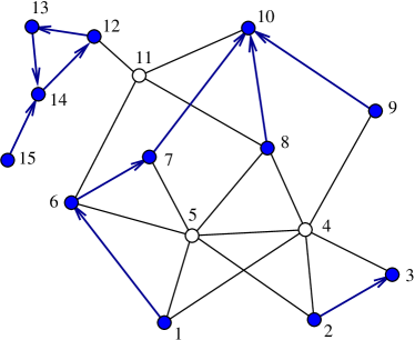
Figure 1: Graphical representation of a microscopic configuration $\{A_{1}=6,A_{2}=3,A_{3}=3,A_{4}=0,A_{5}=0,A_{6}=7,A_{7}=10,A_{8}=10,A_{9}=10,A_{10}=10,A_{11}=0,A_{12}=13,A_{13}=14,A_{14}=12,A_{15}=14\}$ for a small graph with $N=15$ vertices. A vertex $i$ is drawn as an open circle if its state $A_{i}=0$, otherwise it is drawn as a filled circle. If the state of vertex $i$ is $A_{i}=j\neq i$, then we add an arrow on the edge $(i,j)$ with this arrow pointing from $i$ to $j$. Vertices $3$ and $10$ are two root vertices, therefore they do not have out-going arrows.

On the other hand, for each cycle-free subgraph of graph $G$, we can randomly assign one vertex (say $i$) of each connected tree component of this subgraph as the root vertex (i.e., setting $A_{i}=i$), then there is a unique way of fixing the state variable $A_{j}$ of all the other vertices $j$ of this tree component. By repeating this assigning process for all the tree components of this cycle-free subgraph and then fixing all the other vertices $k$ not belonging to this subgraph to the un-occupied state $A_{k}=0$, we obtain a solution $\underline{A}$ for the graph $G$.

Consider a legitimate subgraph $G_{T}$ of the graph $G$ which is formed by trees and c-trees. Is there a one-to-one correspondence between $G_{T}$ and a solution $\underline{A}$ of the graph $G$? The answer is no. Each subgraph $G_{T}$ corresponds to many solutions of graph $G$. To explain this, let us assume $G_{T}$ is composed of a non-empty set of trees and a non-empty set of c-trees. For each tree $t\in G_{T}$, we can randomly choose a vertex of this tree as the root vertex and then fix all the other vertices. The total number of different configurations for this tree is therefore equal to the total number $|t|$ of vertices in tree $t$. For each c-tree $c\in G_{T}$ there are two ways of fixing the arrow directions for the edges on the cycle, therefore the total number of different configurations for this c-tree is simply $2$. From these discussions we know that each legitimate subgraph $G_{T}$ of the graph $G$ corresponds to

$$\mathcal{C}(G_{T})\equiv 2^{n_{c}(G_{T})}\prod\limits_{{\rm tree}\ t\in G_{T}}|t|$$ (4)

different solutions $\underline{A}$ of $G$, where $n_{c}(G_{T})$ is the total number of c-trees in the subgraph $G_{T}$. The number $\mathcal{C}(G_{T})$ can be regarded as the degree of degeneracy of the legitimate subgraph $G_{T}$.

After we have defined a state variable for each vertex, we can define a partition function for the system as

$$Z(x)=\sum\limits_{\underline{A}}\exp\Bigl{[}x\sum\limits_{i=1}^{N}(1-\delta_{A_{i}}^{0})w_{i}\Bigr{]}\prod\limits_{(i,j)\in G}C_{ij}(A_{i},A_{j})\;,$$ (5)

where $w_{i}\geq 0$ is the fixed weight of each vertex $i$, and $x$ is a positive re-weighting parameter. Due to the product term of edge factors, only microscopic configurations satisfying all the edges of $G$ have non-zero contributions to the partition function. The re-weighting parameter $x$ favors microscopic configurations with more occupied vertices and larger total weights.

The partition function can also be expressed as a sum over all the legitimate subgraphs $G_{T}$:

$$Z(x)=\sum\limits_{G_{T}}\mathcal{C}(G_{T})\exp\bigl{[}xW(G_{T})\bigr{]}\;,$$ (6)

where $W(G_{T})\equiv\sum_{i\in G_{T}}w_{i}$ means the total weight of vertices in the subgraph $G_{T}$. Notice that, for two legitimate subgraphs $G_{T}$ and $G_{T}^{\prime}$ of identical total weight $W$, their contributions to the partition function will be different if $\mathcal{C}(G_{T})\neq\mathcal{C}(G_{T}^{\prime})$. In other words, the partition function $Z(x)$ does not weight uniformly all the legitimate subgraphs of the same total weight $W$ but favors those legitimate subgraphs $G_{T}$ with larger degrees of degeneracy $\mathcal{C}(G_{T})$. We are not much worried by this bias issue, since the minimum FVS problem corresponds to the $x\gg 1$ limit of our partition function. At the limit of large $x$, the partition function $Z(x)$ is contributed exclusively by the legitimate subgraphs of maximum total weight, and the small differences among the degrees of degeneracy of these subgraphs become unimportant.

Let us define the free entropy $\Phi(x)$ of the spin glass system as

$$\Phi(x)=\frac{1}{x}\ln Z(x)\;.$$ (7)

For a graph $G$ containing a large number $N$ of vertices, we expect the free entropy $\Phi(x)$ to be an extensive thermodynamic quantity, namely $\Phi(x)\simeq N\phi(x)$. The free entropy density $\phi(x)$ does not depend on $N$ in the thermodynamic limit of $N\rightarrow\infty$.

4 Replica-symmetric mean field theory

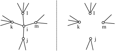
Figure 2: A simple explanation on the Bethe-Peierls approximation. The central vertex $i$ on the left panel is connected to several other vertices ($\partial i=\{j,k,m,l\}$ in this example). Vertex $i$ mediates strong correlations among the states of these neighboring vertices. If vertex $i$ is removed from the graph (right panel), these neighboring vertices no longer feel the common effect from vertex $i$ but they may still be correlated due to other remaining paths of the graph. As a simplest approximation we ignore all the possible remaining correlations and assume that the vertices in set $\partial i$ are mutually independent of each other when vertex $i$ is removed.

Consider a randomly chosen vertex $i$ of the graph $G$, and denote by $q_{i}^{A_{i}}$ the marginal probability that this vertex takes the state $A_{i}$. The vertex $i$ may be connected to some other vertices of the graph (see for example the left panel of Figure 2), and its state $A_{i}$ is then influenced greatly by the states of these neighboring vertices. In return the states of the vertices in the neighboring vertex set $\partial i$ are also strongly influenced by the state $A_{i}$ of vertex $i$. To avoid over-counting in computing the marginal probability $q_{i}^{A_{i}}$ of vertex $i$, it is helpful for us to first remove vertex $i$ from the graph and consider all the possible vertex state combinations of the set $\partial i$ in the remaining system (referred to as a cavity graph, see the right panel of Figure 2). In this cavity graph the vertices of set $\partial i$ might still be correlated, but in our mean field treatment we neglect all these possible correlations and assume independence of probabilities. This approximation is commonly known as the Bethe-Peierls approximation Bethe-1935 ; Peierls-1936 ; Peierls-1936a ; Mezard-Montanari-2009 in the statistical physics community.

Let us denote by $P_{\backslash i}(\{A_{j}:j\in\partial i\})$ as the state joint probability distribution of the neighboring vertices of vertex $i$ in the cavity graph (where vertex $i$ has been removed). In our mean field treatment this joint probability distribution is then approximated by the following factorized form:

$$P_{\backslash i}(\{A_{j}:j\in\partial i\})\approx\prod\limits_{j\in\partial i}q_{j\rightarrow i}^{A_{j}}\;,$$ (8)

where $q_{j\rightarrow i}^{A_{j}}$ denotes the marginal probability distribution of the state $A_{j}$ of vertex $j\in\partial i$ in the cavity graph, where the effect of vertex $i$ is not considered.

If all the vertices $j\in\partial i$ are either empty ($A_{j}=0$) or are roots ($A_{j}=j$) in the cavity graph, then vertex $i$ can be a root ($A_{i}=i$) when it is added to the graph. This is because a neighboring vertex $j$ can adjust its state to $A_{j}=i$ after vertex $i$ is added even if its state is $A_{j}=j$ in the cavity graph. Similarly, if one vertex $l\in\partial i$ is occupied in the cavity graph and all the other vertices of set $\partial i$ are either empty or are roots in the cavity graph, then vertex $i$ can take the state $A_{i}=l$ when it is added to the graph. These considerations, together with the Bethe-Peierls approximation (8), lead to the following expressions for the marginal probability $q_{i}^{A_{i}}$:

$$q_{i}^{0} = \frac{1}{z_{i}}\;,$$ (9)

$$q_{i}^{i} = \frac{e^{xw_{i}}\prod\limits_{j\in\partial i}\bigl{(}q_{j\rightarrow i}^{0}+q_{j\rightarrow i}^{j}\bigr{)}}{z_{i}}\;,$$ (10)

$$q_{i}^{l} = \frac{e^{xw_{i}}(1-q_{l\rightarrow i}^{0})\prod\limits_{k\in\partial i\backslash l}\bigl{(}q_{k\rightarrow i}^{0}+q_{k\rightarrow i}^{k}\bigr{)}}{z_{i}}\;,\quad l\in\partial i\;$$

where the normalization constant $z_{i}$ is calculated by

$$z_{i} \equiv 1+e^{xw_{i}}\times\biggl{[}\prod\limits_{j\in\partial i}\bigl{(}q_{j\rightarrow i}^{0}+q_{j\rightarrow i}^{j}\bigr{)}+$$ (12)

$$\quad\sum\limits_{j\in\partial i}(1-q_{j\rightarrow i}^{0})\prod\limits_{k\in\partial i\backslash j}\bigl{(}q_{k\rightarrow i}^{0}+q_{k\rightarrow i}^{k}\bigr{)}\biggr{]}\;.$$

In the above expressions, $\partial i\backslash j$ means the set of all the neighboring vertices of vertex $i$ except vertex $j$.

After the marginal probabilities $q_{i}^{A_{i}}$ for all the vertices $i$ have been obtained, the mean fraction of occupied vertices $\rho$ is easily calculated through

$$\rho=1-\frac{1}{N}\sum\limits_{i=1}^{N}q_{i}^{0}\;,$$ (13)

and the relative total weight of the occupied vertices $\omega$ is obtained through

$$\omega\equiv\frac{1}{N}\sum\limits_{i=1}^{N}(1-q_{i}^{0})w_{i}\;.$$ (14)

Under the Bethe-Peierls approximation the free entropy $\Phi(x)$ has the following simple expression:

$$\Phi(x)=\sum\limits_{i=1}^{N}\phi_{i}-\sum\limits_{(i,j)\in G}\phi_{ij}\;,$$ (15)

where $\phi_{i}$ and $\phi_{ij}$ are, respectively, the free entropy contribution of a vertex $i$ and an edge $(i,j)$:

$$\phi_{i} = \frac{1}{x}\ln\biggl{[}1+e^{xw_{i}}\prod\limits_{j\in\partial i}[q_{j\rightarrow i}^{0}+q_{j\rightarrow i}^{j}]+$$ (16)

$$\quad e^{xw_{i}}\sum\limits_{j\in\partial i}(1-q_{j\rightarrow i}^{0})\prod\limits_{k\in\partial i\backslash j}(q_{k\rightarrow i}^{0}+q_{k\rightarrow i}^{k})\biggr{]}\;,$$

$$\phi_{ij} = \frac{1}{x}\ln\biggl{[}q_{i\rightarrow j}^{0}q_{j\rightarrow i}^{0}+(1-q_{i\rightarrow j}^{0})(q_{j\rightarrow i}^{0}+q_{j\rightarrow i}^{j})+$$ (17)

$$\quad(1-q_{j\rightarrow i}^{0})(q_{i\rightarrow j}^{0}+q_{i\rightarrow j}^{i})\biggr{]}\;.$$

The free entropy expression (15) can be rigorously justified from the mathematical framework of partition function expansion Zhou-Wang-2012 ; Xiao-Zhou-2011 ; Zhou-etal-2011 or through the cluster variation method Kikuchi-1951 ; An-1988 . From (15) the free entropy density is then obtained as $\phi(x)=\frac{1}{N}\Phi(x)$. The entropy density $s$ of the system is then calculated through

$$s=x(\phi-\omega)\;.$$ (18)

To complete the mean field theory we also need a set of equations for the probability distributions $q_{i\rightarrow j}^{A_{i}}$. Since $q_{i\rightarrow j}^{A_{i}}$ has the same meaning as $q_{i}^{A_{i}}$ but is defined on the cavity graph where vertex $j$ is being removed, we can write down the following equations under the Bethe-Peierls approximation:

$$q_{i\rightarrow j}^{0} = \frac{1}{z_{i\rightarrow j}}\;,$$ (19)

$$q_{i\rightarrow j}^{i} = \frac{e^{xw_{i}}\prod\limits_{k\in\partial i\backslash j}\bigl{(}q_{k\rightarrow i}^{0}+q_{k\rightarrow i}^{k}\bigr{)}}{z_{i\rightarrow j}}\;,$$ (20)

$$q_{i\rightarrow j}^{l} = \frac{e^{xw_{i}}(1-q_{l\rightarrow i}^{0})\prod\limits_{m\in\partial i\backslash j,l}\bigl{(}q_{m\rightarrow i}^{0}+q_{m\rightarrow i}^{m}\bigr{)}}{z_{i\rightarrow j}}\;,\quad l\in\partial i\backslash j\;$$

where $\partial i\backslash j,l$ means the set of all the neighboring vertices of vertex $i$ except vertex $j$ and vertex $l$, and the normalization constant $z_{i\rightarrow j}$ is expressed as

$$z_{i\rightarrow j} \equiv 1+e^{xw_{i}}\biggl{[}\prod\limits_{k\in\partial i\backslash j}\bigl{(}q_{k\rightarrow i}^{0}+q_{k\rightarrow i}^{k}\bigr{)}+$$ (22)

$$\sum\limits_{k\in\partial i\backslash j}(1-q_{k\rightarrow i}^{0})\prod\limits_{m\in\partial i\backslash j,k}\bigl{(}q_{m\rightarrow i}^{0}+q_{m\rightarrow i}^{m}\bigr{)}\biggr{]}\;.$$

These self-consistent equations are commonly referred to as a set of belief propagation (BP) equations in the literature.

The BP equations and the free entropy expression (15) form the replica-symmetric (RS) mean field theory of the spin glass model (5). For a single graph instance $G$, we can iterate the BP equations on the edges of the graph at a fixed value of re-weighting parameter $x$. If the BP equations are able to converge to a fixed point, we can then calculate the entropy density $s$, the occupation density $\rho$ and the relative total weight of occupied vertices $\omega$ at this fixed point. The value $1-\rho$ is then the fraction of un-occupied vertices estimated by the RS mean field theory. Because some occupied vertices of the c-trees need to be included into the FVS besides all the un-occupied vertices, this fraction $1-\rho$ is regarded as a lower-bound on the fraction of vertices in the FVS.

The RS mean field theory can also be used to calculate ensemble-averaged properties. Let us first consider the ensemble of finite-connectivity Erdös-Rényi (ER) random graphs. Such an ensemble is characterized by a mean vertex degree $c$ and a Poisson degree distribution

$$P(d)=\frac{e^{-c}c^{d}}{d!}\;,$$ (23)

which gives the probability that a randomly chosen vertex $i$ has $d$ edges attached He-Liu-Wang-2009 . We create a large population array of two-dimensional elements $(q_{i\rightarrow j}^{0},q_{i\rightarrow j}^{i})$ to represent the messages on all the edges of a random graph. This population array is then updated until the distribution of elements in the array no longer changes with time. We then keep updating the population to compute through the mean field expressions the thermodynamic quantities such as $\rho$, $\omega$, $\phi$, and $s$. For simplicity we set the weight $w_{i}$ of each vertex $i$ to be $w_{i}=1$ in all our following numerical calculations.

In each step of the above-mentioned population updating process, first an integer value $d$ is generated according to the Poisson distribution (23). This value $d$ is considered as the degree of a central vertex, say $i$. We then randomly choose $d$ elements from the population array and consider them as the input messages $(q_{j\rightarrow i}^{0},q_{j\rightarrow i}^{j})$ from the $d$ neighboring vertices $j$ of vertex $i$. Then we obtain $d$ new output messages $(q_{i\rightarrow j}^{0},q_{i\rightarrow j}^{i})$ according to the BP equations and replace $d$ randomly chosen elements of the population array by these $d$ new ones. Such a kind of population dynamics simulations is now commonly used for studying the ensemble-averaged properties of spin glasses, see, for example, the textbook Mezard-Montanari-2009 .

Figure 3 shows the mean field results for the ER random graph ensemble with mean degree $c=10$. The occupation density $\rho$ increases with re-weighting parameter $x$ (Figure 3), while the entropy density $s$ decreases with $x$ and becomes negative at $x>14$ (Figure 3). The entropy density $s$ as a function of occupation density $\rho$ is shown in Figure 3, which appears to be concave.

If the entropy density $s$ is positive even at $x\rightarrow\infty$, we take the value of $\rho=\rho_{0}$ at $x\rightarrow\infty$ as the maximal occupation density the system can achieve. On the other hand, if the calculated entropy density $s$ becomes negative at large values of $x$, since the true entropy density of a spin glass system with discrete state variables should be non-negative, the point $\rho=\rho_{0}$ at which $s(\rho_{0})=0$ is regarded as the maximum value of occupation density the system can achieve.

In random graphs, since the typical cycle length diverges logarithmically with the vertex number $N$, the correction effect of the single cycle of each c-tree to the FVS size will be of order at most $[\ln N]^{-1}$. Therefore these correction effects can be safely neglected in the thermodynamic limit of $N\rightarrow\infty$. The fraction of vertices in the minimum feedback vertex sets is then obtained as $1-\rho_{0}$ for the random graph ensemble.

At mean degree $c=10$ the mean field results of Figure 3 suggest that $\rho_{0}\approx 0.517$, namely each minimum FVS contains about $0.483N$ vertices of the random graph. The minimum FVS size as predicted by the RS mean field theory is shown in Figure 4 as a function of mean vertex degree $c$ (the cross symbols). As expected, the minimum FVS size increases continuously with $c$.

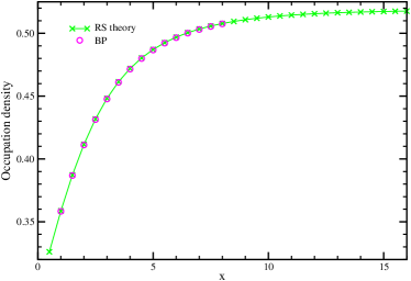
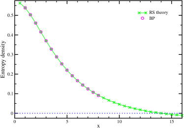
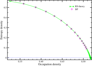
Figure 3: Replica-symmetric mean field results on ER random graphs of mean degree $c=10$. Cross symbols are ensemble-averaged results, while circles are results obtained by BP iteration on a single random graph instance of $N=10^{5}$ vertices. (a) Mean occupation density $\rho$. (b) Entropy density $s$. (c) Entropy density $s$ as a function of occupation density $\rho$ obtained by eliminating the re-weighting parameter $x$ from each pair of points $(x,\rho)$ and $(x,s)$ of (a) and (b). The dotted lines of (b) and (c) indicate $s=0$. BP iteration fails to converge at $x\geq 8$ on the single graph instance.

We can also perform BP simulations on single random graph instances. A single ER random graph instance can be easily generated by the following way: start from an empty graph of $N$ vertices and zero edges, we keep adding an edge to two randomly chosen different vertices until the total number of edges in the graph reaches $M=(c/2)N$ (of cause, self-connections and multiple edges between the same pair of vertices are discarded). For such a large single random graph instance, we find that if the BP iteration process is able to converge to a fixed point, the occupation density $\rho$ and the entropy density $s$ calculated at this fixed point coincide with the ensemble-averaged values. However, if the mean degree $c>=4$ and the re-weighting parameter $x$ is large, the BP iteration process fails to converge to a fixed point. For example, in the case of $c=10$ our preliminary results suggest that BP iteration is not convergent when $x\geq 8$ (see Figure 3).

The non-convergence of BP on single random graph instances (with mean degree $c\geq 4$) at large values of $x$ indicates that the RS mean field theory is not sufficient to describe the FVS problem at high occupation densities. We need to consider correlations among the states of the neighboring vertices of each given vertex $i$, and the Bethe-Peierls approximation Eq. (8) has to be improved. This can be achieved by applying the first-step replica-symmetry-breaking (1RSB) mean field theory Mezard-Parisi-2001 ; Zhou-Wang-2012 ; Xiao-Zhou-2011 ; Zhou-etal-2011 . We will return to this issue and the related spin glass phase transition problem in a future paper.

We also work on the ensemble of regular random graphs. In a regular random (RR) graph, each of the vertices has exactly $K$ edges but the graph is otherwise completely random. The RS mean field predictions on the minimum FVS size of this RR graph ensemble are shown in Figure 4. At each value of degree $K$ the RS prediction slightly exceeds the mathematical lower-bound obtained by Bau and co-authors Bau-Wormald-Zhou-2002 .

5 Belief propagation-guided decimation

The RS mean field theory can also guide us to construct feedback vertex sets for single graph instances. We have implemented a simple belief propagation-guided decimation (BPD) algorithm as follows:

1. Input a graph G and initialize randomly the edge messages $(q_{i\rightarrow j}^{0},q_{i\rightarrow j}^{i})$ and $(q_{j\rightarrow i}^{0},q_{j\rightarrow i}^{j})$ for each edge $(i,j)$ of the graph $G$. The feedback vertex set $\Gamma$ is initialized to be empty. The re-weighting parameter $x$ is set to an appropriate value (e.g., $x\approx 10$).

2. Perform the BP iteration process a number $T$ of rounds (in each round of the iteration, the vertices of the graph $G$ are randomly ordered and their output messages are then updated sequentially). A fixed point of BP equations may not be reached after these $T$ rounds of iteration. No matter whether a BP fixed point has reached, we compute the empty probability $q_{i}^{0}$ of each vertex $i$ based on the current inputting messages to vertex $i$. Then the $fN$ vertices with the highest empty probability values are added to the set $\Gamma$, and these vertices are then removed from the graph $G$ together with all the edges attached to them.

3. Then we further simplify the graph $G$ by recursively removing vertices of degree $0$ or $1$ until all the remaining vertices of the graph have two or more attached edges. Notice that these removed vertices are not added to the set $\Gamma$.

4. If the graph $G$ is non-empty, we repeat the above-mentioned step (1) and step (2).

5. Output the resulting set $\Gamma$.

During the decimation process, if the remaining graph still contains cycles, at least one vertex will be moved to the set $\Gamma$ to decrease the number of cycles. The BPD process will terminate only when no cycles are present in the remaining graph. Therefore the set $\Gamma$ is a feedback vertex set of $G$. In other words, the subgraph of $G$ obtained by removing all the vertices of $\Gamma$ is a forest (there are usually many tree components in this forest but no c-trees).

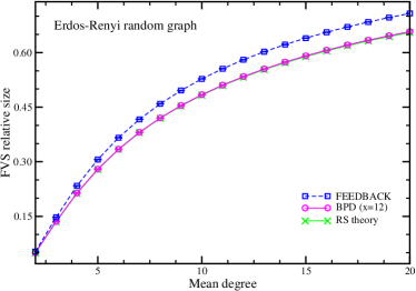
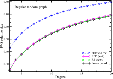
Figure 4: Comparing the theoretical predictions and algorithmic results on the minimum FVS sizes. (a) Erdös-Rényi random graphs; (b) regular random graphs. Cross symbols are the RS mean field predictions; circle symbols (together with error bars) are the average values of the FVS sizes obtained by a single run of the BPD algorithm on $96$ random graph instances of $N=10^{5}$ vertices; square symbols (together with error bars) are the average values of the FVS sizes obtained by a single run of the FEEDBACK algorithm Bafna-Berman-Fujito-1999 on the same $96$ random graph instances. The re-weighting parameter of the BPD is fixed to $x=12$ in the case of ER graphs, and to $x=7$ in the case of RR graphs. The mathematical lower-bounds on the FVS size of RR graphs (see the third column of Table 2 in Bau-Wormald-Zhou-2002 ) are shown as plus symbols in (b).

We have implemented the above BPD algorithm using C++ programming language (the code is freely available upon request). In our numerical simulations we set the BPD parameters to be $T=500$ and $f=0.01$. These parameters are not necessarily optimal but are chosen so that a single run of the BPD algorithm on a large graph instance of $N=10^{5}$ vertices and $M=10^{6}$ edges will terminate within three to four hours. If the fraction $f$ is further reduced, say to $f=0.001$, then the BPD algorithm will reach slightly smaller feedback vertex sets, but the computing time is much longer.

We have tested the performance of the BPD algorithm at different fixed values of the re-weighting parameter $x$. The sizes of the constructed feedback vertex sets $\Gamma$ only change very slightly with different choices of $x$. For ER random graphs the value of $x=12$ seems to be close to optimal, while for regular random graphs the value is $x=7$.

The results of this BPD algorithm on ER and RR graphs are shown in Figure 4 and  4, respectively (the circle symbols). As a comparison we also show in the same figure the results obtained by the well-known FEEDBACK algorithm of Bafna and co-workers Bafna-Berman-Fujito-1999 (the square symbols). The FEEDBACK is a fast heuristic algorithm that is guaranteed to construct a FVS of size not exceeding two times that of an optimal FVS.

We can clearly see from Figure 4 that the sizes of feedback vertex sets constructed by the BPD algorithm reach the predicted minimum FVS sizes of the RS mean field theory. On the other hand, for a given random graph instance, the feedback vertex sets constructed by the FEEDBACK algorithm are extensively larger in size than those constructed by the BPD algorithm. The good agreement between the results of the BPD algorithm and the mean field predictions indicates that the BPD algorithm is excellent for random graph instances, and it also indicates that the RS mean field theory is very good in predicting the mean minimum FVS sizes of random graphs (the predictions can be further improved slightly if ergodicity-breaking is considered in the theory).

We have also applied the BPD algorithm on hyper-cubic regular lattices with periodic boundary conditions. For two-dimensional square lattices the feedback vertex sets obtained by the BPD algorithm ($x=7$) contain about $35.1\%$ of the vertices. This value is very close to the mathematical lower-bound of $\frac{1}{3}$ obtained by Beineke and Vandell Beineke-Vandell-1997 ; Bau-Wormald-Zhou-2002 and is much better than the value of $49.5\%$ obtained by the FEEDBACK algorithm. For three-dimensional cubic lattices the feedback vertex sets obtained by the BPD algorithm ($x=7$) contain about $41.9\%$ of the vertices, which is again very close to the mathematical lower-bound of $\frac{2}{5}$ Beineke-Vandell-1997 ; Bau-Wormald-Zhou-2002 and much better than the value of $49.9\%$ obtained by the FEEDBACK algorithm. The performance of the BPD algorithm may be further improved if we consider explicitly the correlation effect of short loops in the iteration equations (see Zhou-Wang-2012 for example). A systematic comparison of the performance of BPD with other optimization algorithms (such as simulated annealing and parallel tempering) needs to be carried out in the future.

6 Conclusion and discussions

We have constructed a spin glass model (5) for the feedback vertex set problem on an undirected graph. We have solved this model by replica-symmetric mean field theory on the ensemble of finite-connectivity random graphs. We have also implemented a belief propagation-guided decimation algorithm based on this mean field theory and applied this algorithm to single random graph instances and hyper-cubic regular lattices. Our numerical results of Figure 4 demonstrate that the BPD message-passing algorithm is able to construct nearly optimal feedback vertex sets for single random graph instances and regular lattice instances. The BPD algorithm also has much better performance than the conventional FEEDBACK algorithm of Bafna-Berman-Fujito-1999 when applied to finite-dimensional hyper-cubic lattices.

Although the replica-symmetric mean field theory appears to predict the minimum FVS sizes of Erdös-Rényi random graphs very well, the BP iteration process does not converge to a fixed point on single random graphs when the re-weighting parameter $x$ exceeds certain threshold value. We still need to carry out the replica-symmetry-broken mean field calculations to fully understand the statistical physics properties of the spin glass model (5) at large $x$ values. Such a theoretical exploration is deferred to a later publication.

The FVS problem of directed graphs is even more important in practical applications. A way of constructing a Ising model for the directed FVS problem has been suggested in the recent paper of Lucas Lucas-2013 . Following the idea of Ref. Lucas-2013 (and also that of Ref. Bayati-etal-2008 ) we may define on each vertex $i$ of a directed graph $G$ an integer height state $h_{i}$ such that $h_{i}=0$ means vertex $i$ is un-occupied (belonging to the FVS) and $h_{i}\geq 1$ means $i$ is occupied (not belonging to the FVS). A height configuration of the whole system can be denoted as $\underline{h}\equiv\{h_{1},h_{2},\ldots,h_{N}\}$. On each directed edge $(i\rightarrow j)$ pointing from vertex $i$ to vertex $j$, a simple edge factor $C_{i\rightarrow j}$ similar to Eq. (3) can be introduced as

$$C_{i\rightarrow j}(h_{i},h_{j})=\delta_{h_{j}}^{0}+\bigl{(}1-\delta_{h_{j}}^{0}\bigr{)}\Theta(h_{j}-h_{i})\;,$$ (24)

where $\Theta(n)=0$ for integer $n\leq 0$ and $\Theta(n)=1$ for integer $n\geq 1$. If $h_{i}\times h_{j}=0$ then $C_{i\rightarrow j}(h_{i},h_{j})=1$; if $h_{i}\geq 1$ and $h_{j}\geq 1$ (namely both $i$ and $j$ are occupied) then $C_{i\rightarrow j}(h_{i},h_{j})=1$ only if $h_{i}<h_{j}$. A partition function similar to Eq. (5) can be defined on the directed graph $G$ as

$$Z(x)=\sum\limits_{\underline{h}}\exp\Bigl{[}x\sum\limits_{i=1}^{N}(1-\delta_{h_{i}}^{0})w_{i}\Bigr{]}\prod\limits_{(i\rightarrow j)\in G}C_{i\rightarrow j}(h_{i},h_{j})\;.$$ (25)

Because of the product term of edge factors in the above equation, if there is a directed cycle within the subgraph of occupied vertices, the corresponding height configuration $\underline{h}$ will have zero contribution to the partition function.

For the ensemble of directed ER random graphs in which each vertex on average having $\alpha$ inputting edges and $\alpha$ out-going edges, our preliminary RS mean field calculations indicate that at $\alpha=10.0$ a minimum feedback vertex set contains about $0.448N$ vertices. A detailed report of the mean field and algorithmic results will be presented in a later paper.

References

- (1) S. A. Cook. The complexity of theorem-proving procedures. In P. M. Lewis, M. J. Fischer, J. E. Hopcroft, A. L. Rosenberg, J. W. Thatcher, and P. R. Young, editors, Proceedings of the 3rd Annual ACM Symposium on Theory of Computing, pages 151–158, New York, 1971. ACM.
- (2) R. M. Karp. Reducibility among combinatorial problems. In E. Miller, J. W. Thatcher, and J. D. Bohlinger, editors, Complexity of Computer Computations, pages 85–103, New York, 1972. Plenum Press.
- (3) M. Garey and D. S. Johnson. Computers and Intractability: A Guide to the Theory of NP-Completeness. Freeman, San Francisco, 1979.
- (4) L. W. Beineke and R. C. Vandell. Decycling graphs. J. Graph Theory, pages 59–77, 1997.
- (5) D. Zöbel. The deadlock problem: a classifying bibliography. SIGOPS Oper. Syst. Rev., 17(4):6–15, 1983.
- (6) B. Fiedler, A. Mochizuki, G. Kurosawa, and D. Saito. Dynamics and control at feedback vertex sets. I: Informative and determining nodes in regulatory networks. Journal of Dynamics and Differential Equations, 25:563–604, 2013.
- (7) A. Mochizuki, B. Fiedler, G. Kurosawa, and D. Saito. Dynamics and control at feedback vertex sets. II: A faithful monitor to determine the diversity of molecular activities in regulatory networks. J. Theor. Biol., 335:130–146, 2013.
- (8) Y.-Y. Liu, J.-J. Slotine, and A.-L. Barabási. Controllability of complex networks. Nature, 473:167–173, 2011.
- (9) Y.-Y. Liu, J.-J. Slotine, and A.-L. Barabási. Observability of complex systems. Proc. Natl. Acad. Sci. USA, 110:2460–2465, 2013.
- (10) G. Bianconi and M. Marsili. Loops of any size and Hamilton cycles in random scale-free networks. J. Stat. Mech.: Theor. Exp., P06005, 2005.
- (11) E. Marinari, R. Monasson, and G. Semerjian. An algorithm for counting circuits: Application to real-world and random graphs. Europhys. Lett., 73:8–14, 2006.
- (12) E. Marinari and G. Semerjian. On the number of circuits in random graphs. J. Stat. Mech.: Theor. Exp., P06019, 2006.
- (13) E. Marinari, G. Semerjian, and V. Van Kerrebroeck. Finding long cycles in graphs. Phys. Rev. E, 75:066708, 2007.
- (14) G. Bianconi and N. Gulbahce. Algorithm for counting large directed loops. J. Phys. A: Math. Theor., 41:224003, 2008.
- (15) Da-Ren He, Zong-Hua Liu, and Bing-Hong Wang. Complex Systems and Complex Networks. Higher Education Press, Beijing, 2009.
- (16) M. Bayati, C. Borgs, A. Braunstein, J. Chayes, A. Ramezanpour, and R. Zecchina. Statistical mechanics of steiner trees. Phys. Rev. Lett., 101:037208, 2008.
- (17) M. Bailly-Bechet, C. Borgs, A. Braunstein, J. Cheyes, A. Dagkessamanskaia, J.-M. Francois, and R. Zecchina. Finding undetected protein associations in cell signaling by belief propagation. Proc. Natl. Acad. Sci. USA, 108:882–887, 2011.
- (18) I. Biazzo, A. Braunstein, and R. Zecchina. Performance of a cavity-method-based algorithm for the prize-collecting steiner tree problem on graphs. Phys. Rev. E, 86:026706, 2012.
- (19) H. A. Bethe. Statistical theory of superlattices. Proc. R. Soc. London A, 150:552–575, 1935.
- (20) R. Peierls. Statistical theory of superlattice with unequal concentrations of the components. Proc. R. Soc. London A, 154:207–222, 1936.
- (21) R. Peierls. On Ising’s model of ferromagnetism. Proc. Camb. Phil. Soc., 32:477–481, 1936.
- (22) M. Mézard and A. Montanari. Information, Physics, and Computation. Oxford Univ. Press, New York, 2009.
- (23) H.-J. Zhou and C. Wang. Region graph partition function expansion and approximate free energy landscapes: Theory and some numerical results. J. Stat. Phys., 148:513–547, 2012.
- (24) J.-Q. Xiao and H.-J. Zhou. Partition function loop series for a general graphical model: free-energy corrections and message-passing equations. J. Phys. A: Math. Theor., 44:425001, 2011.
- (25) H.-J. Zhou, C. Wang, J.-Q. Xiao, and Z. Bi. Partition function expansion on region-graphs and message-passing equations. J. Stat. Mech.: Theo. Exp., L12001, 2011.
- (26) R. Kikuchi. A theory of cooperative phenomena. Phys. Rev., 81:988–1003, 1951.
- (27) G. An. A note on the cluster variation method. J. Stat. Phys., 52:727–734, 1988.
- (28) M. Mézard and G. Parisi. The Bethe lattice spin glass revisited. Eur. Phys. J. B, 20:217–233, 2001.
- (29) S. Bau, N. C. Wormald, and S.-M. Zhou. Decycling numbers of random regular graphs. Random Struct. Alg., 21:397–413, 2002.
- (30) V. Bafna, P. Berman, and T. Fujito. A -approximation algorithm for the undirected feedback vertex set problem. SIAM J. Discrete Math., 12:289–297, 1999.
- (31) A. Lucas. Ising formulations of many NP problems. e-print arXiv:1302.5841, 2013.