Abstract

The spectrum of radially excited hadrons provides much information about the confinement forces in QCD. The confinement is realized most naturally in terms of the QCD string whose quantization gives rise to the radially excited modes. We propose an alternative framework for the description of the excited spectrum. Namely we put forward some effective field models in which the hadrons acquire masses due to interaction with a scalar field modeling the non-perturbative gluon vacuum. The effective potential for this field is periodic with an infinite number of non-equivalent vacua. The radially excited hadrons emerge as elementary excitations over different vacua. We construct explicit examples for such effective theories in the meson sector. An interesting byproduct of the considered models is the existence of a classical field configuration in each vacuum. Depending on the model, it can represent a domain wall, Nielsen-Olesen vortex or ’t Hooft–Polyakov monopole. In the pure scalar sector, it is shown that the first quantum correction leads to splitting of the radially excited modes into two nearly degenerate states. Such a phenomenon has some phenomenological support. The presented approach may be also viewed as an alternative framework to the bottom-up AdS/QCD models where the radial excitations appear on the classical level as well.

1 Introduction

A large number of observed hadron resonances can be interpreted as the radial excitations of some lighter hadrons due to identical quantum numbers. The form of spectrum of the radial excitations is determined by the confinement forces in Quantum Chromodynamics (QCD). Thus the study of radial excitations seems to be indispensable to the understanding of the confinement dynamics.

The quark confinement and the radial excitations arise naturally in the hadron string models where the string serves as an approximation for the gluon flux-tube with nearly massless quarks at the ends [1, 2]. This relativistic approach is well accommodated for the description of light mesons representing ultrarelativistic systems. The hadron strings usually imply that the limit of large number of colors $N_{c}$ in QCD [3] is taken. The meson excitations become narrow, and hence well defined objects for the theoretical study, with the masses being approximately independent of $N_{c}$. In addition, the radial spectrum must contain an infinite number of states. The semiclassical quantization of a thin flux-tube typically gives a linearly rising spectrum for masses squared [2, 4],

$$M_{k}^{2}=a(k+b),\qquad k=0,1,2,\dots,$$ (1)

where the slope $a$ is proportional to the string tension. Since the latter is governed by the gluodynamics, the slope $a$ is expected to be unaffected by the quantum numbers of meson resonances. The known spectrum of light mesons seems to agree with the behavior (1) [5, 6].

The concept that QCD in the large-$N_{c}$ limit may be formulated as some string theory has been evolving for some decades. The usual models based on the QCD string possess a nice basic feature: The linear Regge recurrence, $m_{J}^{2}\sim J$ ($J$ denotes the hadron spin), emerges already on the classical level of rotating string. The radial modes appear after quantization. Unfortunately, a consistent theory of quantized QCD string has not been built in spite of extensive efforts. It is therefore interesting to look for alternative dynamical approaches leading to the relation (1) in some natural way, at least approximately. The term ”natural” we understand in a specific way: It would be interesting to construct a model where the relation (1) holds on the classical level, like the relation $m_{J}^{2}\sim J$ in the rotating string. In this case, one can hope to escape the problems related to the rigorous quantization. In some sense, an example of such a model is given by the five-dimensional soft-wall holographic model [7]. We wish to construct an example staying within the four-dimensional framework.

In fact, a careful analysis of existing data shows that a stronger statement than the recurrence (1) can be made: The light non-strange mesons cluster near certain equidistant values of energy squared with repeating structure of the clusters [6, 8, 9, 10, 11], see, e.g., figure in Appendix A. The matter looks as if the underlying dynamics recurred periodically when one moves to higher energies. This observation suggests that as a starting point for the model building we may take an assumption that the gluon vacuum has the periodic structure in a dynamical sense.

In the present paper, we put forward a new dynamical approach to the description of the radial hadron excitations. The approach is based on a realization of the aforementioned assumption within the framework of an effective field theory. We construct models in which the mesons acquire masses via a Higgs-like mechanism due to interaction with a scalar field $\varphi$. The central idea is that the effective potential for $\varphi$ is periodic and its vacua are non-equivalent. This leads to the appearance of infinite set of vacuum expectation values $\langle\varphi\rangle_{k}$, $k=0,1,2,\dots$. Correspondingly, the hadron fields coupled to $\varphi$ can have different mass terms depending on the choice of $\langle\varphi\rangle_{k}$, i.e. depending on the scale we probe the theory. As a consequence, each hadron has an infinite discrete set of masses $M_{k}$, the states with $k>0$ are identified with the radial excitations of the ground state having $k=0$.

Needless to say that this approach proposes a new viewpoint on the nature of the radially excited hadrons. Perhaps the following mechanical analogy clarifies the essence of our idea. Consider the mathematical pendulum with a friction. Depending on the energy of push, it will oscillate near its equilibrium position after $k$ turns. The energy of hadron creation corresponds to the energy of push in this rough analogy and the ”winding number” $k$ does to the radial number of the created hadron. An interesting byproduct of the considered models is the existence of non-trivial classical solutions which will be analyzed in detail.

The paper is organized as follows. In Sect. 2, we construct an effective model of single scalar field which possesses an infinite number of non-degenerate vacua. This model is used in Sect. 3 to describe the radial spectrum of the vector mesons. The emerging vortex-line solutions are discussed in detail. The quantum correction to the scalar model of Sect. 2 is analyzed in Sect. 4. The Sect. 5 contains discussions concerning the phenomenology of the proposed model and possible connections of our approach with effective models for QCD. Our conclusions and some prospects for future work are presented in Sect. 6.

2 Scalar theory with non-degenerate vacua

Consider the following effective field theory for a real scalar field in four dimensions,

$$\mathcal{L}=\frac{1}{2}\partial_{\mu}\varphi\partial^{\mu}\varphi+\frac{\mu^{4}}{2\lambda}\left[\cos\left(\frac{\lambda}{\mu^{2}}\varphi^{2}-2\pi b\right)-\cos(2\pi b)\right],$$ (2)

where $\mu$ has the dimension of mass and the parameters $\lambda$ and $b$ are dimensionless. The periodicity of the interaction term in (2) imposes a restriction on the value of parameter $b$: the interval $0\leq b<1$ covers all nontrivial cases. For instance, the case $b=1$ is equivalent to the $b=0$ one, etc. The parameter $\lambda$ plays the role of coupling constant. In the weak coupling regime, $|\lambda|\ll 1$, the Lagrangian (2) reduces to the scalar theory $\lambda\varphi^{4}$,

$$\mathcal{L}_{|\lambda|\ll 1}=\frac{1}{2}\partial_{\mu}\varphi\partial^{\mu}\varphi+\frac{1}{2}\mu^{2}\sin(2\pi b)\varphi^{2}-\frac{\lambda}{4}\cos(2\pi b)\varphi^{4}+\mathcal{O}(\lambda^{2}\varphi^{6}).$$ (3)

As is seen from (3), the parameter $b$ induces the mass term except the cases $b=0$ and $b=\frac{1}{2}$. We could introduce the mass term $\frac{1}{2}m^{2}\varphi^{2}$ from the very beginning and set $b=0$. This theory would be completely equivalent. We find the variant (2) more convenient for our purposes because the parameter $b$ will have then a direct meaning of intercept in the relation (1). The expansion (3) shows also that the energy functional is bounded from below in the weak coupling regime if $\lambda\cos(2\pi b)>0$. This results in the following interrelation between the sign of the coupling $\lambda$ and the value of $b$: $0\leq b<\frac{1}{4}$ or $\frac{3}{4}\leq b<1$ for $\lambda>0$ and $\frac{1}{4}\leq b<\frac{3}{4}$ for $\lambda<0$.

At $b=0$ the Lagrangian (2) resembles the sine-Gordon model [12]. The model (2), however, is quite different since the nonlinear power of $\varphi$ in the cosine destroys the translational invariance (modulo a general factor) $\varphi\rightarrow\varphi+2\pi k$, $k=0,\pm 1,\pm 2,\dots$. The vacua are therefore non-equivalent, although they deliver equal minima to the action.

The potential in (2) is minimized on the constant field configurations

$$\langle\varphi\rangle_{k}=\sqrt{\frac{2\pi\mu^{2}}{\lambda}(k+b)},\qquad k=0,1,2,\dots.$$ (4)

Consider small perturbations around the vacua (4),

$$\varphi=\langle\varphi\rangle_{k}+\sigma(x).$$ (5)

The quadratic part of the Lagrangian for $\sigma$ reads

$$\mathcal{L}_{\sigma}^{(2)}=\frac{1}{2}\partial_{\mu}\sigma\partial^{\mu}\sigma-\lambda\langle\varphi\rangle_{k}^{2}\sigma^{2}.$$ (6)

The spectrum of excitations follows from (6) and (4),

$$M^{2}_{\sigma,k}=2\lambda\langle\varphi\rangle_{k}^{2}=4\pi\mu^{2}(k+b),$$ (7)

which has the Regge-like form (1). Thus the considered model has an infinite number of unconnected vacua with different excitation energies given by the relation (7).

It is worth mentioning that a simple semiclassical quantization of the gluon string with massless quarks confined by the linear potential leads to the relation [4]: $M^{2}_{k}=4\pi\tau k+\text{const}$, where $\tau$ denotes the string tension. The mass parameter $\mu^{2}$ has thus an analogy with the string tension.

The seeming similarity of the Lagrangian (2) with the sine-Gordon model poses an interesting question whether there exist some soliton-like solutions in the two-dimensional case. In fact, the most close analogue to the sine-Gordon model is provided by the following modification of the Lagrangian (2),

$$\tilde{\mathcal{L}}=\frac{1}{2}\partial_{\mu}\varphi\partial^{\mu}\varphi+\frac{\mu^{6}}{\lambda^{2}\varphi^{2}}\left[\cos\left(\frac{\lambda}{\mu^{2}}\varphi^{2}\right)-1\right].$$ (8)

The minima of effective potentials in (8) and in (2) at $b=0$ coincide. As $\lambda\rightarrow 0$ we obtain the theory

$$\tilde{\mathcal{L}}=\frac{1}{2}\partial_{\mu}\varphi\partial^{\mu}\varphi-\frac{1}{2}\mu^{2}\varphi^{2}+\frac{1}{4!}\frac{\lambda^{2}}{\mu^{2}}\varphi^{6}+\dots,$$ (9)

where the mass term arises from the cosine as in the sine-Gordon model [12]. The equation of motion for the field $\varphi$ in the Lagrangian (8) has a soliton-like solution which in the static case takes the form

$$\varphi=\pm 2\sqrt{\frac{\mu^{2}}{\lambda}\arctan{e^{2\mu(x-x_{0})}}}.$$ (10)

The expression in (10) represents nothing but the square root of the static one-soliton solution in the sine-Gordon model [12]. The solution (10), however, is not a genuine soliton. This conclusion follows from the absence of the Bäcklund transformations for the system (8). In the relativistic systems described by the Lagrangians $\mathcal{L}=\frac{1}{2}(\partial_{\mu}\varphi)^{2}-V(\varphi)$, the necessary condition for the existence of the Bäcklund transformations is [13]: $V^{\prime\prime\prime}+\alpha^{2}V^{\prime}=0$, where $\alpha$ is a parameter and the prime denotes derivative. This condition is not fulfilled in the model (8). The solution (10) describes a usual kink, which connects two neighbouring vacua, and in four dimensions it becomes a domain wall. The same situation takes place in the model (2), where the kinks exist but cannot be found analytically.

3 Abelian Higgs model with periodic potential

Consider now a $U(1)$ gauge model of the Nielsen-Olesen type [14] in which the Higgs potential is taken from the scalar model (2). The Lagrangian reads

$$\mathcal{L}=D_{\mu}\varphi(D^{\mu}\varphi)^{*}+\frac{\mu^{4}}{2\lambda}\left[\cos\left(\frac{2\lambda}{\mu^{2}}\varphi\varphi^{*}-2\pi b\right)-\cos(2\pi b)\right]-\frac{1}{4}F_{\mu\nu}F^{\mu\nu},$$ (11)

where

$$\varphi=\frac{\varphi_{1}+i\varphi_{2}}{\sqrt{2}},\qquad D_{\mu}\varphi=\partial_{\mu}\varphi-ieA_{\mu}\varphi,\qquad F_{\mu\nu}=\partial_{\mu}A_{\nu}-\partial_{\nu}A_{\mu}.$$ (12)

The scalar field $\varphi$ acquires non-zero vacuum expectation values (v.e.v.) (4). Pointing these values along the $\varphi_{1}$, we will have an infinite set of massive fields $\varphi_{1}$ and massless fields $\varphi_{2}$ which represent the Goldstone modes, one for each vacuum in the absence of the gauge field $A_{\mu}$. The Goldstone modes are transformed into the longitudinal degrees of freedom of the gauge field due to the Higgs mechanism. This can be easily demonstrated by the standard change of the field variables,

$$V_{\mu}=A_{\mu}-\frac{\partial_{\mu}\eta(x)}{e\langle\varphi\rangle_{k}},\qquad\varphi=\frac{\langle\varphi\rangle_{k}+\sigma(x)}{2}\exp\left({\frac{i\eta(x)}{\langle\varphi\rangle_{k}}}\right).$$ (13)

In terms of the variables (13), the quadratic part of the Lagrangian (11) is cast into the canonical form,

$$\mathcal{L}_{\sigma,V}^{(2)}=\frac{1}{2}\partial_{\mu}\sigma\partial^{\mu}\sigma-\frac{1}{2}M^{2}_{\sigma}\sigma^{2}-\frac{1}{4}F_{\mu\nu}F^{\mu\nu}+\frac{1}{2}M^{2}_{V}V_{\mu}V^{\mu}+\text{const},$$ (14)

where $M^{2}_{\sigma}$ is given by (7) and the masses of gauge field over different vacua become

$$M^{2}_{V,k}=e^{2}\langle\varphi\rangle_{k}^{2},\qquad k=0,1,2\dots.$$ (15)

The relations (7) and  (15) demonstrate that the infinite towers of massive vector and scalar particles emerge. It is straightforward to generalize the model to the case of the gauge group $SU(2)$, see Appendix B.

Let us seek for the Nielsen–Olesen vortex solutions. The equations of motion for the Lagrangian (11) are:

$$D^{\mu}D_{\mu}\varphi=-\mu^{2}\varphi\sin\left(\frac{2\lambda}{\mu^{2}}\varphi\varphi^{*}-2\pi b\right),$$ (16)

$$\partial^{\nu}F_{\mu\nu}=ie(\varphi^{\ast}\partial_{\mu}\varphi-\varphi\partial_{\mu}\varphi^{*})+2e^{2}A_{\mu}\varphi\varphi^{*}.$$ (17)

We will consider the static case, with the gauge choice $A_{0}=0$. Following the paper [14] we look for a cylindrically symmetric solution, with axis along the $z$-direction. The corresponding ansatz is [14]

$$\vec{A}(\vec{r})=\frac{\vec{r}\times\vec{e}_{z}}{r}A(r),\qquad\varphi(\vec{r})=\chi(r)e^{in\theta},$$ (18)

where $\vec{e}_{z}$ denotes a unit vector along the $z$-direction and $n$ is an integer. In addition, it is assumed that $A_{\theta}=A(r)$ and $A_{r}=A_{z}=0$. The flux is given by $\Phi(r)=2\pi rA(r)$ so that the magnetic field is

$$B(r)=\frac{\Phi^{\prime}(r)}{2\pi r}=\frac{(rA(r))^{\prime}}{r},$$ (19)

where the prime stays for the derivative with respect to $r$. Inserting this ansatz to the equations of motion we arrive at

$$\frac{\left(r\chi^{\prime}\right)^{\prime}}{r}-\left[\left(\frac{n}{r}-eA\right)^{2}+\mu^{2}\sin\left(\frac{2\lambda}{\mu^{2}}\chi^{2}-2\pi b\right)\right]\chi=0,$$ (20)

$$\left(\frac{\left(rA\right)^{\prime}}{r}\right)^{\prime}-2\chi^{2}\left(Ae^{2}-\frac{ne}{r}\right)=0.$$ (21)

The exact solution of this system cannot be obtained analytically. We are going to find a solution with asymptotic behavior on the spacial infinity of the type $\chi\simeq\text{const}$. It is rather clear that the constant should be proportional to the vacuum expectation value of the field $\varphi$. Treating $\chi$ as a constant we get from the equation (21), with $C$ a constant of integration and $K_{\nu}$ the modified Bessel function of the second kind,

$$A_{k}(r)=\frac{n}{er}+\frac{C}{e}K_{1}\left(e\langle\varphi\rangle_{k}r\right)=\frac{n}{er}+\frac{C}{e}\sqrt{\frac{\pi}{2e\langle\varphi\rangle_{k}r}}\,e^{-e\langle\varphi\rangle_{k}r}+\dots.$$ (22)

Then the magnetic field is

$$B_{k}=-C\langle\varphi\rangle_{k}rK_{0}\left(e\langle\varphi\rangle_{k}r\right)=-C\sqrt{\frac{\pi\langle\varphi\rangle_{k}}{2er}}\,e^{-e\langle\varphi\rangle_{k}r}+\dots.$$ (23)

Here the dots mean the lower order terms at $r\rightarrow\infty$. Substituting the asymptotics (22) for $A_{k}(r)$ into the equation (20) we obtain the approximate solution $\chi_{k}\simeq\langle\varphi\rangle_{k}/\sqrt{2}$, which defines the characteristic length $\Lambda$ (meaning the penetration length of the magnetic field in the condensed matter physics), $\Lambda_{k}=(e\chi_{k})^{-1}$. In contrast to the Nielsen–Olesen theory [14], here one formally has an infinite number of characteristic lengths, however, the real physical penetration length is determined by the largest one corresponding to $k=0$.

We thus see that each vacuum possesses not only its own spectrum but also its own vortex (or monopole in the $SU(2)$ case, see Appendix B). As was demonstrated in [14] the vortex-lines have a flux-tube structure and move according to the equation of motion of the Nambu dual string. A simple estimation shows [14] that the energy density of such a flux-tube is proportional to $\langle\varphi\rangle^{2}$, i.e. the energy density of the vortex-line in the $k$-th vacuum is given by the relation (4). On the other hand, the dimensional analysis of the energy functional corresponding to the Lagrangian (11) shows that the vortex mass is fixed, $M_{\text{vor}}\sim\frac{\mu}{\lambda}$ [14]. This means that the cross-section of the $(k+1)$-th vortex is squeezed by the factor $k$.

4 Quantum correction

The interaction in the Lagrangian (2) is non-renormalizable in four dimensions. It is well known that for the effective field theories the renormalizability is a desirable but not necessary property because these theories are often considered as approximations valid in the tree level only. Nevertheless, the analysis of the first quantum corrections in the non-renormalizable effective models may occasionally lead to unexpected insights into some observable effects. In any case, it is interesting to compare the impact of the first quantum correction to the model (2) with that of the $\lambda\varphi^{4}$ scalar theory with the spontaneous symmetry breaking.

A convenient formalism for the calculation of quantum corrections is based on the effective potential. For the theory of one scalar field, the expansion of the potential in the Planck constant is given by  [16]

$$V_{\text{eff}}=V(\varphi_{\text{cl}})+\hbar\frac{(V^{\prime\prime}(\varphi_{\text{cl}}))^{2}}{64\pi^{2}}\left(-\frac{3}{2}+\ln\frac{V^{\prime\prime}(\varphi_{\text{cl}})}{\mathcal{M}^{2}}\right)+\mathcal{O}(\hbar^{2}),$$ (24)

where $V$ is the classical potential expanded on the field configuration $\varphi_{\text{cl}}$ minimizing the classical action. For the Lagrangian (2) one has,

$$V(\varphi_{\text{cl}})=-\frac{\mu^{4}}{2\lambda}\left(\cos\left(\frac{\lambda}{\mu^{2}}\varphi_{\text{cl}}^{2}-2\pi b\right)-\cos(2\pi b)\right),$$ (25)

where the second derivative of $V$ reads

$$V^{\prime\prime}(\varphi_{\text{cl}})=\mu^{2}\left(2\frac{\lambda}{\mu^{2}}\varphi_{\text{cl}}^{2}\cos\left(2\pi b-\frac{\lambda}{\mu^{2}}\varphi_{\text{cl}}^{2}\right)-\sin\left(2\pi b-\frac{\lambda}{\mu^{2}}\varphi_{\text{cl}}^{2}\right)\right).$$ (26)

In our natural units, we must of course set $\hbar=1$. The quantum correction induces the dependence of effective potential (24) on the energy scale $\mathcal{M}$. This scale will be regarded as a new mass parameter of the model.

A typical behavior of the effective potential for a particular choice of $\lambda$ and $\mathcal{M}$ is displayed in Fig. 1. The quantum correction to the first minimum (hence, to the mass of the ground state) is very close to the case of the $\lambda\varphi^{4}$ scalar theory with the spontaneous symmetry breaking [16]. But after the second minimum a qualitative change of the picture occurs: The quantum correction splits each minimum of the classical potential into two new nearly degenerate minima. This means the quantum doubling of the radially excited states. It is important that the new minima lie higher than the first minimum. This property also has a direct interpretation: The more massive is the radial excitation, the more is it unstable. In order to achieve this correct physical picture, the parameter $\mathcal{M}$ must not exceed the typical hadronic scale, $\mathcal{M}\lesssim 1$ GeV (a concrete boundary value slightly depends on $\lambda$).

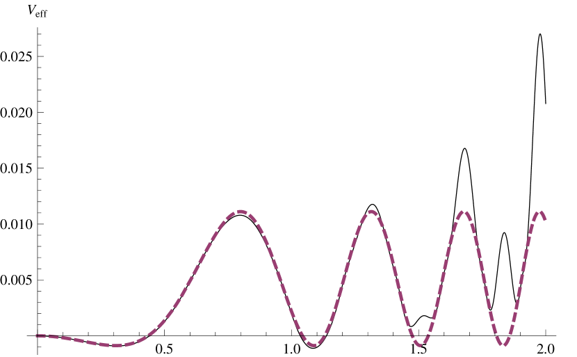
Figure 1: The effective potential (24) (solid line) and the classical potential (25) (dashed line) at $\lambda=-0.4$. The parameters are taken from the trajectory of $f_{0}$-mesons in Fig. 2: $\mu^{2}=0.07$ GeV², $b=1.41$ and we set $\mathcal{M}=0.5$ GeV.

The calculation of the first quantum correction to the vector model of Sect. 3 is much more complicated. But our tentative estimations show that a similar phenomenon of quantum doubling will take place. The predicted phenomenon is difficult to observe because of overlapping decay widths of highly excited resonances. But it is interesting to notice that in some cases, when the available data is rich enough and the neighboring resonances are relatively narrow, a similar doubling is indeed observed in the spectroscopy of the light mesons. The case of $f_{2}$-mesons in the figure of Appendix A demonstrates such a phenomenon. In terms of the quark model, the doubling can have a simple explanation [10]: Two nearly degenerate identical resonances may represent the states with different angular momentum $L$ of the quark-antiquark pair. For instance, the vector mesons can have $L=0$ and $L=2$ and these states are nearly degenerate due to the mass dependence $M_{n,L}\sim n+L$ [10]. The degeneracy here takes place for the radial number $n\geq 2$, i.e. beginning from the third minimum as in Fig. 1. If the so-called polarization data is available (see Bugg’s review in Ref. [5]), even the broad resonances can be, in principle, distinguished. An example is given by the heaviest $\omega_{3}$-meson in the figure of Appendix A. In the case of the scalar mesons, the source of doubling can arise from the mixing with the $s\bar{s}$ scalar states ($s$ denotes the strange quark) [5]. The scalar mesons with the dominant $s\bar{s}$-component are not displayed in Appendix A.

5 Discussions

We have built an example of effective field model describing the infinite radial spectrum of the scalar and vector particles. This infinite spectrum can be accompanied by an infinite number of topological vertices reminiscent of the dual strings. The particle spectrum and topological solutions coexist and it is not clear whether there is a deep sense in this coexistence or the classical solutions represent just an artefact of the model. The original Nielsen–Olesen’s idea [14] was to identify the vortex-line solution with the Nambu dual string. The quantization of the latter had to give rise to the excited hadron spectrum. We deal with a quite different situation: The spectrum of excitations emerges on the classical level and each state can be accompanied by a vortex. This approach avoids all notorious problems with quantization of the hadron strings. The existence of vortices might be speculatively interpreted as a footprint of real QCD string. A precise meaning of this interpretation is then needed. The mass of the excited state cannot be related with the mass of the corresponding vortex since the latter mass is universal for all vacua. The mass of the $n$-th excitation is rather proportional to the sum of masses of $n+1$ vortices which can be created in the vacua below the given energy scale (see the discussions at the end of Sect. 3). In this sense, the $n$-th radial excitation might be interpreted as ”consisting of” $n+1$ vortices. This would give a ”dual” explanation for the fact that, contrary to the expectations from the QCD string models, the size of the radial excitations do not grow with $n$. In terms of the hadron strings, one observes a ”quantization” of the energy density in the gluon flux-tube rather than a ”quantization” of its length with a constant energy density. In other words, the vortices could provide a classical viewpoint on the spatial structure of the excited mesons.

From the phenomenological point of view, the model under consideration predicts a linear Regge-like spectrum for radially excited scalar and vector states. In the general situation, the slopes are different in contrast to the hadron string models where the universal slope is determined by the gluodynamics. The existing experimental data on the light non-strange mesons seems to agree with the approximate universality of slopes of radial meson trajectories within the experimental errors [5]. We can easily incorporate this universality by setting $e^{2}=2\lambda$ in the mass relations (7) and (15). But this entails a complete degeneracy of the scalar and vector states. If we associate the scalar field $\varphi$ with the scalar isoscalar particles ($f_{0}$-mesons) and the vector field with the vector isoscalar states ($\omega$-mesons) this prediction is not far from the reality, see Fig. 1.

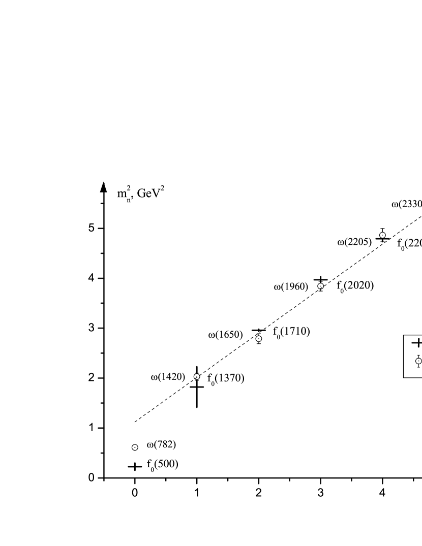
Figure 2: The spectrum of $f_{0}$ and $\omega$ mesons [15]. The vertical size displays the experimental uncertainty. Other states $f_{0}$ reported by the Particle Data [15] are assumed to belong to the $s\bar{s}$-trajectory where the strange component dominates [5]. The state $\omega(2290)$ [15] is identified with the $\omega(2330)$-meson.

If we wish to keep the universal slope but remove the degeneracy we can simply introduce the mass term for the vector field in the Lagrangian (11) and consider a real scalar field. This is tantamount to adding the vector part,

$$\mathcal{L}_{v}=-\frac{1}{4}F_{\mu\nu}F^{\mu\nu}+\frac{1}{2}(m_{v}^{2}+e^{2}\varphi^{2})A_{\mu}A^{\mu},$$ (27)

to the Lagrangian (2). The vector field $A_{\mu}$ in (27) can be also $SU(2)$ massive gauge field carrying the isospin one.

The fact that the field $\varphi$ is scalar does not imply that it should describe the scalar quark-antiquark states. It looks more natural to interpret the field $\varphi$ and its periodic potential as an effective model for the non-perturbative gluon vacuum in QCD. The spectrum of the Lagrangian (2) represents the scalar glueballs in this interpretation. The relation (7) gives the Regge-like form for this spectrum. All quarkonia in the sector of light quarks get masses mainly through interaction with the vacuum field $\varphi$. The quark-antiquark scalar mesons should be then treated in the same fashion as the vector ones in the model (27), i.e. the simplest Lagrangian for a scalar quarkonium $f$ is

$$\mathcal{L}_{s}=\frac{1}{2}\partial_{\mu}f\partial^{\mu}\!f-\frac{1}{2}(m_{s}^{2}+g_{s}^{2}\varphi^{2})f^{2},$$ (28)

which should be added to the Lagrangian (2). Here $f$ is a scalar or pseudoscalar field which can be both isosinglet and isotriplet. The bare mass $m_{s}$ must depend on quantum numbers in order to provide different intercepts for the radial meson trajectories [5]. The approximate universality of slopes entails universality of couplings $g_{s}^{2}\simeq e^{2}\simeq 2\lambda$.

The higher spin mesons can be also introduced by the Lagrangian (28) in which $f$ will denote a higher-spin (HS) field. It represents a totally symmetric traceless tensor of rank $J$, where $J$ denotes the spin of particle [19]. The kinetic and mass term will have additional contributions due to different ways for contracting the Lorentz indices. The hadron strings predict the Regge behavior $M^{2}\sim J$ which is well seen in the observed spectrum of hadrons [5, 6]. This behavior can be incorporated by assuming that the mass term is proportional to the number of physical degrees of freedom $2J+1$ (i.e. each degree of freedom contributes to the bare mass as the scalar field in (28)). The model will contain interactions of HS fields with the excitations of the vacuum field. This is a problem because a self-consistent theory of interacting HS fields is absent. However, if we are interested in the mass spectrum which is supposedly determined by the quadratic part of the action, this problem does not appear.

The models discussed above should be viewed as effective models for QCD in the large-$N_{c}$ limit (because the number of resonances is infinite and the zero-width approximation is implied). They are complementary to the usual effective field theories for the strong interactions (the sigma-models, chiral perturbation theory, etc). The precise sense of complementarity is as follows. The standard effective models are low-energy ones, i.e. they are usually defined below the characteristic scale of the spontaneous chiral symmetry breaking (CSB) — about 1 GeV — and their input parameters are supposed to arise from integration of the degrees of freedom above this scale. In our case, the situation is opposite — by assumption, the input parameters (first of all the bare masses in (27) and (28)) originate from integration of the low-energy degrees of freedom below 1 GeV. A phenomenological support for such a viewpoint comes from the observation that the linear ansatz (1) for the radial meson spectrum is a reasonable approximation for the excited states, while the ground ones below 1 GeV deviate substantially from the linear trajectory. This is seen, for example, in Fig. 1. The deviation is the most pronounced in the pseudoscalar channel [5]. Below 1 GeV, the physics of strong interactions is shaped by the CSB. The building of the low-energy effective theories is therefore guided by the chiral symmetry. Above 1 GeV, the CSB is not crucial [11] and the physics is governed by the gluodynamics. QCD in the large-$N_{c}$ limit represents (assuming that confinement persists in this limit) a theory of an infinite number of narrow and stable non-interacting mesons and glueballs [3] which should appear in the classical effective action. The models considered above satisfy these basic properties.

The interest to the physics of radially excited hadrons has recently been raised due to a fast development of the five-dimensional holographic approach to QCD. Specifically, the Regge-like spectrum (1) is reproduced within the so-called Soft-Wall model [7]. Exploring the gauge/gravity duality from the string theory, the holographic models identify the excited hadrons with the Kaluza-Klein excitations. Our approach is alternative to the holographic one and also attempts to realize a certain concept of duality. Namely, the proposed models are constructed in the spirit of the so-called ”dual QCD” approach born by the Nielsen–Olesen paper [14] (the history and achievements of this line of research are briefly reviewed in Ref. [20]). Within this approach, one tries to reformulate QCD in the long-distance limit as some weakly-coupled ”dual” theory which should describe the non-perturbative physics of the strong interactions. Unfortunately, no connection between the ”dual” variables and the QCD ones has been derived. Thus any model based on the ”dual QCD” represents a purely phenomenological approach. Being aware of theoretical difficulties we would dare nevertheless to outline a possible way for finding certain connections with QCD. It should be reminded that the concept of duality (in the sense of equivalence of two theories plus the strong–weak coupling correspondence) first emerged in the two-dimensional field theories. A spectacular example is given by the duality between the quantized sine-Gordon model and the Thirring model discovered by Coleman [12]. It would be extremely interesting to establish an approximate fermionic theory, bosonization of which leads to our models. This may shed light on the problem of emergence of considered models from QCD since such a fermionic theory can serve as a toy-model for the effective theory of QCD obtained after integrating out the gluonic degrees of freedom.

6 Conclusions and outlook

We have proposed a novel Lagrangian description for the radially excited mesons. The main assumption of our scheme is that the non-perturbative vacuum of QCD has periodic structure in energy scale. The radially excited states appear as elementary excitations over different non-equivalent vacua. The Regge-like form of their spectrum represents, by construction, the main feature of the model and is a consequence of the vacuum periodicity. Each vacuum contains a non-trivial topological configuration which accompanies the corresponding radial excitation. To some extend, the considered models lead to the quantum doubling of the radially excited states and to the linearity of the scalar glueball trajectory. Both phenomena have a certain phenomenological support.

There are many questions which can be (and hopefully will be) addressed within the introduced field models. We mention some of them. (i) The precise relation between the excited mesons and the accompanying classical solutions. (ii) The construction of equivalent fermionic models. (iii) The calculation of the first quantum correction to the vector spectrum. (iv) The influence of non-trivial external conditions (especially the non-zero temperature and finite density) on the whole set of the radially excited mesons. (v) Since the sine-Gordon model has interesting applications in the condensed matter physics and the Nielsen–Olesen theory does in cosmology (cosmic strings), the model of Sect. 2 may have applications in the first field and the model of Sect. 3 may have in the second one.

Appendix A: Meson clusters

In this Appendix, we reproduce the figure from review [9] showing the known spectrum of the light non-strange mesons [15]. The experimental uncertainties are indicated and purely established states are not shaded. The positions of meson clusters (first described in Ref. [8]) are marked by the vertical dashed lines.

Appendix B: Non-Abelian extensions

The construction of the non-Abelian extensions for the model of Sect. 3 is straightforward. We will consider the case of the gauge group $SU(2)$. Let the scalar field $\varphi$ transform according to the real vector representation. The extension of the Lagrangian (11) takes then the form

$$\mathcal{L}=-\frac{1}{4}F_{\mu\nu}^{a}(F^{\mu\nu})^{a}+\frac{1}{2}(D^{\mu}\varphi^{a})(D_{\mu}\varphi^{a})\\ +\frac{\mu^{4}}{2\lambda}\left[\cos\left(\frac{\lambda}{\mu^{2}}\varphi^{a}\varphi^{a}-2\pi b\right)-\cos(2\pi b)\right],$$ (29)

where $a=1,2,3$ and the field strength and the covariant derivative are defined by

$$F_{\mu\nu}^{a}=\partial_{\mu}A_{\nu}^{a}-\partial_{\nu}A_{\mu}^{a}+g\varepsilon^{abc}A_{\mu}^{b}A_{\nu}^{c},$$

$$D_{\mu}\varphi^{a}=\partial_{\mu}\varphi^{a}+g\varepsilon^{abc}A_{\mu}^{b}\varphi^{c}.$$

The scalar field acquires the non-zero v.e.v.

$$\varphi^{a}\varphi^{a}=\langle\varphi\rangle_{k}^{2}.$$

Consider the small fluctuation of the field $\varphi_{a}$ near its v.e.v.

$$\varphi_{a}=(\varphi_{0})_{a}+\sigma_{a}.$$

The gauge freedom allows to point the vector $\varphi_{0}$ along the third axis,

$$(\varphi_{0})_{a}=\langle\varphi\rangle_{k}\delta_{a3}.$$ (30)

Substituting (30) into the Lagrangian (29) and keeping only the terms quadratic in fields, we arrive at

$$\mathcal{L}_{\sigma,A}^{(2)}=\frac{1}{2}\partial_{\mu}\sigma\partial^{\mu}\sigma-\frac{1}{2}M^{2}_{\sigma}\sigma^{2}-\frac{1}{4}{\mathcal{F}_{\mu\nu}^{a}}({\mathcal{F}^{\mu\nu}})^{a}\\ +\frac{1}{2}M^{2}_{A}\left((A_{\mu}^{1})^{2}+(A_{\mu}^{2})^{2}\right)+\text{const},$$ (31)

where

$$\mathcal{F}_{\mu\nu}^{a}=\partial_{\mu}A_{\nu}^{a}-\partial_{\nu}A_{\mu}^{a},$$

$$M^{2}_{A}=M^{2}_{A^{1}}=M^{2}_{A^{2}}=g^{2}\langle\varphi\rangle_{k}^{2},$$

and the gauge boson $A_{\mu}^{3}$ (corresponding to the unbroken symmetry with respect to rotation around the third axis) remains massless.

Another realization of the Higgs model with the $SU(2)$ gauge group is given by the complex spinor representation of the scalar field,

$$\varphi=\left(\begin{array}[]{c}\frac{\varphi_{1}+i\varphi_{2}}{\sqrt{2}}\\ \frac{\varphi_{3}+i\varphi_{4}}{\sqrt{2}}\\ \end{array}\right).$$

The corresponding Lagrangian is

$$\mathcal{L}=-\frac{1}{4}F_{\mu\nu}^{a}(F^{\mu\nu})^{a}+(D^{\mu}\varphi)^{\dagger}(D_{\mu}\varphi)\\ +\frac{\mu^{4}}{2\lambda}\left[\cos\left(\frac{2\lambda}{\mu^{2}}\varphi\varphi^{\dagger}-2\pi b\right)-\cos(2\pi b)\right],$$ (32)

where

$$F_{\mu\nu}^{a}=\partial_{\mu}A_{\nu}^{a}-\partial_{\nu}A_{\mu}^{a}+g\varepsilon^{abc}A_{\mu}^{b}A_{\nu}^{c},$$

$$D_{\mu}\varphi=\partial_{\mu}\varphi-ig\frac{\tau^{a}}{2}A_{\mu}^{a}\varphi.$$

The classical configurations delivering minimum to the effective potential satisfy the condition

$$\varphi\varphi^{\dagger}=\frac{\langle\varphi\rangle_{k}^{2}}{2}.$$

The v.e.v.’s of the fields are $A_{\mu}^{a}=0$ and

$$\varphi=\left(\begin{array}[]{c}0\\ \frac{\langle\varphi\rangle_{k}}{\sqrt{2}}\\ \end{array}\right).$$

Consider the small scalar excitations over the vacua (the unitary gauge is chosen),

$$\varphi=\left(\begin{array}[]{c}0\\ \frac{\langle\varphi\rangle_{k}+\eta}{\sqrt{2}}\\ \end{array}\right).$$

The quadratic in fields part of the Lagrangian takes the form

$$\mathcal{L}_{\sigma,A}^{(2)}=\frac{1}{2}\partial_{\mu}\sigma\partial^{\mu}\sigma-\frac{1}{2}M^{2}_{\sigma}\sigma^{2}-\frac{1}{4}{\mathcal{F}_{\mu\nu}^{a}}({\mathcal{F}^{\mu\nu}})^{a}+\frac{1}{2}M^{2}_{A^{a}}A_{\mu}^{a}(A^{\mu})^{a}+\text{const},$$ (33)

where the spectrum for $M^{2}_{\sigma}$ coincides with (7) and the vector spectrum is

$$M^{2}_{A^{a}}=\frac{g^{2}\langle\varphi\rangle_{k}^{2}}{4},\qquad k=0,1,2...,\qquad a=1,2,3.$$ (34)

The analysis of classical solution in the isovector case results in the ’t Hooft–Polyakov monopoles. We will reproduce briefly the standard derivation of those solutions.

Consider the static case and set $A_{0}^{a}(\vec{x})=0$ for any $\vec{x}$ and $a$. The equations of motion following from the Lagrangian (29) are

$$D^{i}D_{i}\varphi^{a}=\mu^{2}\varphi^{a}\sin\left(\frac{\lambda}{\mu^{2}}\varphi^{b}\varphi^{b}-2\pi b\right),$$ (35)

$$D_{i}(F^{ij})^{a}=-g\varepsilon^{abc}(D^{j}\varphi^{b})\varphi^{c}.$$ (36)

Let us look for the solutions in the form of the hedgehog ansatz [21],

$$\varphi_{a}=x_{a}\frac{u(r)}{r},\qquad A_{i}^{a}=a(r)\varepsilon_{iab}x_{b},$$ (37)

which after the substitution to Eqs. (35) and (36) leads to the equations,

$$a^{\prime\prime}+4r^{-1}a^{\prime}-3ga^{2}-g^{2}r^{2}a^{3}-g^{2}u^{2}a=gu^{2}r^{-2},$$ (38)

$$u^{\prime\prime}\!+\!2r^{-1}(u^{\prime}\!-\!r^{-1}u)\!-\!2gau\!-\!2g^{2}a^{2}r^{2}u\!-\!\mu^{2}u\sin\left(\!\frac{\lambda}{\mu^{2}}u^{2}\!-\!2\pi b\!\right)\!=\!0.$$ (39)

These equations cannot be solved analytically but it is easy to find the asymptotics of the solutions at large distances,

$$r\rightarrow\infty:\qquad u(r)\propto\langle\varphi\rangle_{k},\qquad a(r)\propto-\frac{1}{gr^{2}}.$$ (40)

In order to extract the physical fields ’t Hooft introduced the following gauge-invariant definition for the field strength tensor [22],

$$\mathcal{F_{\mu\nu}}=\frac{1}{|\varphi|}\varphi_{a}(F^{\mu\nu})^{a}-\frac{1}{g|\varphi|^{3}}\varepsilon^{abc}\varphi_{a}(D_{\mu}\varphi_{b})(D_{\nu}\varphi_{c}).$$ (41)

If one has $\varphi_{a}=|\varphi|(0,0,1)$ in some domain for any gauge transformation then $\mathcal{F_{\mu\nu}}=\partial_{\mu}A_{\nu}^{3}-\partial_{\nu}A_{\mu}^{3}$. The asymptotics of $\mathcal{F_{\mu\nu}}$ in the spatial infinity is

$$\mathcal{F_{\mu\nu}}\rightarrow-\frac{1}{gr^{3}}\varepsilon_{\mu\nu a}x_{a}.$$

Here the symbol $\varepsilon$ is zero if any of four-dimensional indices takes the value 4. We thus obtain the expression for the magnetic field corresponding to the magnetic charge $g_{m}=1/g$,

$$B_{a}(\vec{x})=\frac{x_{a}}{gr^{3}},\qquad r\rightarrow\infty.$$ (42)

It is seen that the vector field extends to the spatial infinity. This is related with the existence of the massless mode (see (31)) which can penetrate via the Bose-condensate of the scalar field. The given observation allows to prove (see, e.g., Ref. [21]) that the hedgehog solution represents the Dirac monopole, i.e. the vector-potential has the form

$$A_{r}=A_{\theta}=0,\qquad A_{\varphi}=\frac{g_{m}}{r}\frac{1-\cos\theta}{\sin\theta}.$$

As in Sect. 3, we thus conclude that for each vacuum there exists its own non-trivial classical field configuration — the ’t Hooft–Polyakov monopole in the case under consideration. The magnetic field created by these monopoles in the spatial infinity is, however, equal for any vacuum.

In the case of the isospinor Higgs field — the model (32) — all gauge fields are massive and located in a domain of the size approximately $1/M_{A}$. The ”magnetic” field in the spatial infinity does not appear in this model and the isospinor hedgehog is not a magnetic monopole. In addition, the isospinor hedgehog is unstable [21].

References

- [1] Y. Nambu, Phys. Rev. D 10, 4262 (1974); A. Casher, H. Neuberger and S. Nussinov, Phys. Rev. D 20, 179 (1979); N. Isgur and J. E. Paton, Phys. Rev. D 31, 2910 (1985).
- [2] D. LaCourse and M. G. Olsson, Phys. Rev. D 39, 2751 (1989); A. Yu. Dubin, A. B. Kaidalov and Yu. A. Simonov, Phys. Lett. B 323, 41 (1994); Yu. S. Kalashnikova, A. V. Nefediev and Yu. A. Simonov, Phys. Rev. D 64, 014037 (2001); T. J. Allen, C. Goebel, M. G. Olsson and S. Veseli Phys. Rev. D 64, 094011 (2001); M. Baker and R. Steinke, Phys. Rev. D 65, 094042 (2002); F. Buisseret, Phys. Rev. C 76, 025206 (2007).
- [3] G. ’t Hooft, Nucl. Phys. B 72, 461 (1974); E. Witten, Nucl. Phys. B 160, 57 (1979).
- [4] M. Shifman, hep-ph/0507246.
- [5] A. V. Anisovich, V. V. Anisovich and A. V. Sarantsev, Phys. Rev. D 62, 051502(R) (2000); D. V. Bugg, Phys. Rept. 397, 257 (2004).
- [6] E. Klempt and A. Zaitsev, Phys. Rept. 454, 1 (2007).
- [7] A. Karch, E. Katz, D. T. Son and M. A. Stephanov, Phys. Rev. D 74, 015005 (2006).
- [8] S. S. Afonin, Eur. Phys. J. A 29, 327 (2006).
- [9] S. S. Afonin, Mod. Phys. Lett. A 22, 1359 (2007).
- [10] S. S. Afonin, Phys. Lett. B 639, 258 (2006); Phys. Rev. C 76, 015202 (2007); Int. J. Mod. Phys. A 22, 4537 (2007); M. Shifman and A. Vainshtein, Phys. Rev. D 77, 034002 (2008).
- [11] L. Ya. Glozman, Phys. Rept. 444, 1 (2007).
- [12] R. Rajaraman, Solitons and Instantons, North-Holland Publishing Company (Amsterdam, New York, Oxford, 1982).
- [13] D. W. McLaughlin and A. C. Scott, J. Math. Phys. 14, 1817 (1973); R. K. Dodd and R. K. Bullough, Proc. Roy. Soc. (London) A 351, 499 (1976).
- [14] H. B. Nielsen and P. Olesen, Nucl. Phys. B 61, 45 (1973).
- [15] J. Beringer et al. (Particle Data Group), Phys. Rev. D 86, 010001 (2012).
- [16] P. Ramond, Field Theory: A Modern Primer, Westview Press (2001); M. E. Peskin, D. V. Schroeder, An Introduction to Quantum Field Theory, Westview Press (1995).
- [17] H. B. Meyer, Glueball Regge trajectories, Ph.D. Thesis [hep-lat/0508002].
- [18] E. Gregory et al., JHEP 1210, 170 (2012).
- [19] L. P. S. Singh and C. R. Hagen, Phys. Rev. D 9, 898 (1974).
- [20] M. Baker and R. Steinke, Phys. Rev. D 63, 094013 (2001).
- [21] A. M. Polyakov, Zh. Eksp. Teor. Fiz. 68, 1975 (1975).
- [22] G. ’t Hooft, Nucl. Phys. B 79, 276 (1974).