When is an axisymmetric potential separable?

Abstract

An axially symmetric potential $\psi(\rho,z)=\psi(r,\theta)$ is completely separable if the ratio $\mathfrak{s}:\mathfrak{k}$ is constant. Here $\mathfrak{s}=r^{-1}\partial_{r}\partial_{\theta}(r^{2}\psi)$ and $\mathfrak{k}=\partial_{\rho}\partial_{z}\psi$. If $\beta=\mathfrak{s}/\mathfrak{k}$, then the potential admits an integral of the form $2I=L^{2}+\beta v_{z}^{2}+2\xi$, where $\xi$ is some function of positions determined by the potential $\psi$. More generally, an axially symmetric potential respects the third axisymmetric integral of motion – in addition to the classical integrals of the Hamiltonian and the axial component of the angular momentum – if there exist three real constants $a,b,c$ (not all simultaneously zero, $a^{2}+b^{2}+c^{2}\neq 0$) such that $a\mathfrak{s}+b\mathfrak{h}+c\mathfrak{k}=0$, where $\mathfrak{h}=r^{-1}\partial_{\sigma}\partial_{\tau}(r\psi)$ and $(\sigma,\tau)$ is the parabolic coordinate in the meridional plane such that $\sigma^{2}=r+z$ and $\tau^{2}=r-z$.

1 introduction

Numerical orbit integrations in realistic potentials indicate that regular orbits are the norms rather than the exceptions in astrophysics. However, only known exact integrals of motion besides those due to the Noether theorem are the separation constants of the Hamilton–Jacobi equation, which are limited to the class of potentials known as the Stäckel potential. None the less, behaviours of regular orbits of most astrophysical interests appear to be well approximated by those found in the Stäckel potential (de Zeeuw, 1985a). Hence, understanding the Stäckel potential is not only the first step to sort out regular orbits but also of practical importance.

Unfortunately, the Stäckel potential is usually defined to be the potential separable in an ellipsoidal (or one of its degenerate limits) coordinate, which hinders easy understanding and somewhat obscures physical meaning. Lynden-Bell (2003) on the other hand presented an elementary derivation of the third integral of motion in axially symmetric potentials using only vector calculus. His idea is based on the realization that the kinetic part of a non-trivial quadratic integral of motion is the scalar product of the angular momenta about two foci. The angular momentum with respect to $z=a$ on the symmetry axis is given by $\mn@boldsymbol{L}_{a}=(\mn@boldsymbol{r}-a{\hat{\Bbbk\mkern-3.0mu}\mkern 3.0mu}{})\mn@boldsymbol{\times}\mn@boldsymbol{v}=\mn@boldsymbol{L}-a({\hat{\Bbbk\mkern-3.0mu}\mkern 3.0mu}{}\mn@boldsymbol{\times}\mn@boldsymbol{v})$, where ${\hat{\Bbbk\mkern-3.0mu}\mkern 3.0mu}{}$ is the unit vector in the direction of the symmetry axis. Hence, the kinetic part considered by him is equivalent to $\mn@boldsymbol{L}_{a}\mn@boldsymbol{\cdot}\mn@boldsymbol{L}_{-a}=L^{2}-a^{2}(v^{2}-v_{z}^{2})$, where $L=\lVert\mn@boldsymbol{L}\rVert$, $v=\lVert\mn@boldsymbol{v}\rVert$ and $v_{z}={\hat{\Bbbk\mkern-3.0mu}\mkern 3.0mu}{}\mn@boldsymbol{\cdot}\mn@boldsymbol{v}$. However, $v^{2}$ is the kinetic part of the Hamiltonian, $\mathcal{H}=\frac{1}{2}v^{2}+\psi$ and the assumption is therefore equivalent to existence of an integral the kinetic part of which is given by $L^{2}+a^{2}v_{z}^{2}$.

Here we explore the condition under which there exists such an integral of motion with the kinetic part of $L^{2}+\beta v_{z}^{2}$. This approach is conceptually advantageous as imaginary magnitudes are replaced by negative constants, and thus unifies the separability in both prolate and oblate spheroidal coordinates into variation of a single real parameter. More importantly, this affords us to express the necessary condition for axially symmetric potentials to admit the third integral without prior knowledge on the constant itself.

In the next section (Sect. 2), we prove that, given the axially symmetric potential $\psi(\rho,z)=\psi(r,\theta)$ where $(\rho,\phi,z)$ and $(r,\theta,\phi)$ are cylindrical and spherical polar coordinates, there exists an integral of motion with its kinetic part given by $L^{2}+\beta v_{z}^{2}$ if (and only if) the ratio of two mixed partial derivatives, $r^{-1}\partial_{r}\partial_{\theta}(r^{2}\psi):\partial_{\rho}\partial_{z}\psi$, is constant (which is the same as $\beta$). An example, namely the Kuzmin (1953) disc potential, is provided in Sect. 3. In Sect. 4, it is shown that this encompasses the Stäckel potentials separable in either prolate or oblate spheroidal coordinate as well as spherical or cylindrical polar coordinate (the location of the coordinate origin is assumed to be known). Discussion on generalization allowing unspecified origin (on the symmetry axis) and separability in the rotational parabolic coordinate follows in Sect. 5. In particular, we find that, by considering the kinetic part of the form $aL^{2}-2b(\mn@boldsymbol{v}\mn@boldsymbol{\times}\mn@boldsymbol{L})\mn@boldsymbol{\cdot}{\hat{\Bbbk\mkern-3.0mu}\mkern 3.0mu}{}+cv_{z}^{2}$, an axially symmetric potential $\psi$ admits the third integral if and only if the null space of three mixed partial derivatives including the earlier two and the third, $r^{-1}\partial_{\sigma}\partial_{\tau}(r\psi)$, is non-trivial (i.e. there exists a constant-coefficient non-trivial linear combination of the three that is identically zero). Here $(\sigma,\tau)$ is the parabolic coordinate in the meridional plane. We conclude in Sect. 6 whilst the Appendices provide an overview of the whole subject concerning separable (Stäckel) potentials and quadratic integrals, which puts the present study on proper wider context.

The treatment here is deliberately elementary, limited to vector calculus and linear algebra whenever possible, except in Sect.  6 and the Appendices. The elliptic and parabolic coordinates are introduced naturally via a modern geometric approach without presumption on any prior knowledge. By contrast, the Appendices, which are independent from the main body, introduce more sophisticated physical and mathematical ideas throughout.

2 proof

Consider a conservative dynamic system governed by Newton’s laws of motion. The motion of a unit-mass tracer is determined by

$$\dot{\mn@boldsymbol{r}}=\mn@boldsymbol{v}\,;\qquad\dot{\mn@boldsymbol{v}}=-\mn@boldsymbol{\nabla}\psi,$$ (1)

where $\psi$ is the potential, which is a scalar function of positions.

The evolution of the angular momentum $\mn@boldsymbol{L}=\mn@boldsymbol{r}\mn@boldsymbol{\times}\mn@boldsymbol{v}$ is then given by $\dot{\mn@boldsymbol{L}}=\cancel{\dot{\mn@boldsymbol{r}}\mn@boldsymbol{\times}\mn@boldsymbol{v}}+\mn@boldsymbol{r}\mn@boldsymbol{\times}\dot{\mn@boldsymbol{v}}=-\mn@boldsymbol{r}\mn@boldsymbol{\times}\mn@boldsymbol{\nabla}\psi$. Thus, for $L^{2}=\lVert\mn@boldsymbol{L}\rVert^{2}=\mn@boldsymbol{L}\mn@boldsymbol{\cdot}\mn@boldsymbol{L}$,

$$\tfrac{1}{2}D_{t}L^{2}=\mn@boldsymbol{L}\mn@boldsymbol{\cdot}\dot{\mn@boldsymbol{L}}=(\mn@boldsymbol{v}\mn@boldsymbol{\times}\mn@boldsymbol{r})\mn@boldsymbol{\cdot}\bigl{(}\mn@boldsymbol{r}\mn@boldsymbol{\times}\mn@boldsymbol{\nabla}\psi\bigr{)}=\mn@boldsymbol{v}\mn@boldsymbol{\cdot}\bigl{[}\mn@boldsymbol{r}\mn@boldsymbol{\times}(\mn@boldsymbol{r}\mn@boldsymbol{\times}\mn@boldsymbol{\nabla}\psi)\bigr{]},$$ (2)

where $D_{t}=\mathrm{d}/\mathrm{d}t$. Let $\mn@boldsymbol{e}^{q}=\mn@boldsymbol{\nabla}q$ and $\partial_{q}=\partial/\partial q$ be the reciprocal frame vector and the partial differential operator. Then $\mn@boldsymbol{\nabla}=\mn@boldsymbol{e}^{r}\partial_{r}+\mn@boldsymbol{e}^{\theta}\partial_{\theta}+\mn@boldsymbol{e}^{\phi}\partial_{\phi}$ in the spherical polar coordinate $(r,\theta,\phi)$ whilst $\set{\hat{\mn@boldsymbol{e}}_{r}=\mn@boldsymbol{e}^{r},\hat{\mn@boldsymbol{e}}_{\theta}=r\mn@boldsymbol{e}^{\theta},\hat{\mn@boldsymbol{e}}_{\phi}=r\sin\theta\,\mn@boldsymbol{e}^{\phi}}$ constitutes the corresponding set of orthonormal frame vectors. Then $D_{t}L^{2}=-2\mn@boldsymbol{v}\mn@boldsymbol{\cdot}\mn@boldsymbol{s}$, where

$$\begin{split}\mn@boldsymbol{s}&=-\mn@boldsymbol{r}\mn@boldsymbol{\times}(\mn@boldsymbol{r}\mn@boldsymbol{\times}\mn@boldsymbol{\nabla}\psi)=r^{2}\mn@boldsymbol{\nabla}\psi-\mn@boldsymbol{r}(\mn@boldsymbol{r}\mn@boldsymbol{\cdot}\mn@boldsymbol{\nabla}\psi)\\ &=r^{2}\bigl{(}\mn@boldsymbol{\nabla}\psi-\mn@boldsymbol{e}^{r}\partial_{r}\psi\bigr{)}=\bigl{(}\mn@boldsymbol{e}^{\theta}\partial_{\theta}+\mn@boldsymbol{e}^{\phi}\partial_{\phi}\bigr{)}(r^{2}\psi).\end{split}$$ (3)

Here we have used $\mn@boldsymbol{r}=r\hat{\mn@boldsymbol{e}}_{r}=r\mn@boldsymbol{e}^{r}$ and $\mn@boldsymbol{e}^{r}\mn@boldsymbol{\cdot}\mn@boldsymbol{e}^{r}=\hat{\mn@boldsymbol{e}}_{r}\mn@boldsymbol{\cdot}\hat{\mn@boldsymbol{e}}_{r}=1$.

Meanwhile, $\dot{v}_{z}=-\partial_{z}\psi$ and thus

$$\tfrac{1}{2}D_{t}v_{z}^{2}=v_{z}\dot{v}_{z}=-\mn@boldsymbol{v}\mn@boldsymbol{\cdot}{\hat{\Bbbk\mkern-3.0mu}\mkern 3.0mu}{}\,\partial_{z}\psi,$$ (4)

where ${\hat{\Bbbk\mkern-3.0mu}\mkern 3.0mu}{}$ is the fixed unit vector in the $z$-direction so that $v_{z}=\mn@boldsymbol{v}\mn@boldsymbol{\cdot}{\hat{\Bbbk\mkern-3.0mu}\mkern 3.0mu}{}$. The set $\set{\hat{\mn@boldsymbol{e}}_{\rho}=\hat{\mn@boldsymbol{e}}_{r}\sin\theta+\hat{\mn@boldsymbol{e}}_{\theta}\cos\theta,\hat{\mn@boldsymbol{e}}_{\phi},{\hat{\Bbbk\mkern-3.0mu}\mkern 3.0mu}{}}$ consists in the orthonormal frame vectors for the cylindrical polar coordinate $(\rho=r\sin\theta,\phi,z=r\cos\theta)$ whilst its reciprocal frame vector set is composed of $\set{\mn@boldsymbol{e}^{\rho}=\hat{\mn@boldsymbol{e}}_{\rho},\mn@boldsymbol{e}^{\phi}=\hat{\mn@boldsymbol{e}}_{\phi}/\rho,\mn@boldsymbol{e}^{z}={\hat{\Bbbk\mkern-3.0mu}\mkern 3.0mu}{}}$ and so $\mn@boldsymbol{\nabla}=\hat{\mn@boldsymbol{e}}_{\rho}\partial_{\rho}+{\hat{\Bbbk\mkern-3.0mu}\mkern 3.0mu}{}\,\partial_{z}+\rho^{-1}\hat{\mn@boldsymbol{e}}_{\phi}\partial_{\phi}$.

Suppose $2Q=L^{2}+\beta v_{z}^{2}$ with a constant $\beta$. Then $\dot{Q}=-\mn@boldsymbol{v}\mn@boldsymbol{\cdot}\mn@boldsymbol{u}$, where

$$\mn@boldsymbol{u}=\mn@boldsymbol{e}^{\theta}\partial_{\theta}(r^{2}\psi)+\mn@boldsymbol{e}^{\phi}\partial_{\phi}(r^{2}\psi)+\beta\,{\hat{\Bbbk\mkern-3.0mu}\mkern 3.0mu}{}\,\partial_{z}\psi.$$ (5)

If $\mn@boldsymbol{u}=\mn@boldsymbol{\nabla}\xi-\mn@boldsymbol{\nabla}\mn@boldsymbol{\times}\mn@boldsymbol{A}$ is the Helmholtz decomposition of the vector field $\mn@boldsymbol{u}$ in equation (5), then $\dot{Q}+\mn@boldsymbol{v}\mn@boldsymbol{\cdot}\mn@boldsymbol{\nabla}\xi=\mn@boldsymbol{v}\mn@boldsymbol{\cdot}(\mn@boldsymbol{\nabla}\mn@boldsymbol{\times}\mn@boldsymbol{A})=(\mn@boldsymbol{v}\mn@boldsymbol{\times}\mn@boldsymbol{\nabla})\mn@boldsymbol{\cdot}\mn@boldsymbol{A}$. Consequently, if $\mn@boldsymbol{u}$ is curl free, then $I=Q+\xi$ is conserved along the motion of the tracer. Since $\mn@boldsymbol{\nabla}\mn@boldsymbol{\times}\mn@boldsymbol{e}^{q}=\mn@boldsymbol{\nabla}\mn@boldsymbol{\times}\mn@boldsymbol{\nabla}q=0$, we have

$$\begin{split}\mn@boldsymbol{\nabla}\mn@boldsymbol{\times}\mn@boldsymbol{u}&=\mn@boldsymbol{e}^{r}\mn@boldsymbol{\times}\mn@boldsymbol{e}^{\theta}\partial_{r}\partial_{\theta}(r^{2}\psi)+\mn@boldsymbol{e}^{r}\mn@boldsymbol{\times}\mn@boldsymbol{e}^{\phi}\partial_{r}\partial_{\phi}(r^{2}\psi)-\beta\,{\hat{\Bbbk\mkern-3.0mu}\mkern 3.0mu}{}\mn@boldsymbol{\times}\mn@boldsymbol{\nabla}(\partial_{z}\psi)\\ &=\hat{\mn@boldsymbol{e}}_{\phi}\left[\frac{1}{r}\frac{\partial^{2}(r^{2}\psi)}{\partial r\partial\theta}-\beta\frac{\partial^{2}\psi}{\partial\rho\partial z}\right]-\frac{\hat{\mn@boldsymbol{e}}_{\theta}}{\rho}\frac{\partial(r^{2}\psi_{\phi})}{\partial r}+\beta\frac{\hat{\mn@boldsymbol{e}}_{\rho}}{\rho}\frac{\partial\psi_{\phi}}{\partial z},\end{split}$$ (6)

where the partial derivatives with respect to $(r,\theta)$ and $(\rho,z)$ are, respectively, in the spherical and cylindrical polar coordinates and $\psi_{\phi}=\partial_{\phi}\psi$, which is consistently defined in both coordinates provided that the $z$-axis coincides. Hence, if $\psi_{\phi}=0$ and

$$\beta=\frac{\partial_{r}\partial_{\theta}(r^{2}\psi)}{r\,\partial_{\rho}\partial_{z}\psi}$$ (7)

is constant, then there exists a scalar function $\xi$ such that

$$2I=L^{2}+\beta v_{z}^{2}+2\xi$$ (8)

is an integral of motion and

$$\mn@boldsymbol{\nabla}\xi=r\hat{\mn@boldsymbol{e}}_{\theta}\frac{\partial\psi}{\partial\theta}\biggr{\rvert}_{r,\phi}+\beta\,{\hat{\Bbbk\mkern-3.0mu}\mkern 3.0mu}{}\frac{\partial\psi}{\partial z}\biggr{\rvert}_{\rho,\phi}.$$ (9)

Here the partial derivatives are done with holding the coordinate variables in the subscripts fixed.

3 Example

Consider the Kuzmin disc (Kuzmin, 1953, 1956) potential:

$$\psi=-\frac{k}{b},\quad b=\sqrt{\rho^{2}+(a+\lvert z\rvert)^{2}}=\sqrt{r^{2}+2ar\lvert\cos\theta\rvert+a^{2}},$$ (10)

which is generated by an infinitesimally thin disc with the surface density $\Sigma(\rho)\propto(a^{2}+\rho^{2})^{-3/2}$ (Toomre, 1963). It is easy to find

$$\frac{\partial^{2}\psi}{\partial\rho\partial z}=-\frac{3k}{b^{5}}\rho(a+\lvert z\rvert);\ \frac{\partial^{2}(r^{2}\psi)}{\partial r\partial\theta}=-\frac{3a^{2}k}{b^{5}}r^{2}(a+r\lvert\cos\theta\rvert)\sin\theta,$$ (11)

and thus the ratio of equation (7) is constant, $\beta=a^{2}$. Therefore, the potential of equation (10) admits an integral that is quadratic to the velocities (e.g., de Zeeuw, 1985b) in the form of equation (8).

The function $\xi$ is a solution of the partial differential equations resulting from equation (9). Using $r\hat{\mn@boldsymbol{e}}_{\theta}=z\hat{\mn@boldsymbol{e}}_{\rho}-\rho\,{\hat{\Bbbk\mkern-3.0mu}\mkern 3.0mu}{}$ and $\partial_{\theta}=z\partial_{\rho}-\rho\partial_{z}$, equation (9) for equation (10) with $\beta=a^{2}$ reduces to

$$\begin{split}\frac{\partial\xi}{\partial\rho}&=z^{2}\frac{\partial\psi}{\partial\rho}-\rho z\frac{\partial\psi}{\partial z}=-\frac{ak\rho\lvert z\rvert}{b^{3}};\\ \frac{\partial\xi}{\partial z}&=(a^{2}+\rho^{2})\frac{\partial\psi}{\partial z}-\rho z\frac{\partial\psi}{\partial\rho}=\frac{z}{\lvert z\rvert}\frac{ak}{b^{3}}\bigl{[}\rho^{2}+a(a+\lvert z\rvert)\bigr{]}\end{split}$$ (12)

in the cylindrical polar coordinate. Note that the compatibility condition $\partial_{z}(\partial_{\rho}\xi)=\partial_{\rho}(\partial_{z}\xi)$ is satisfied (i.e. eq. 6 being zero), and so the solution $\xi(\rho,z)$ exists. Let us next suppose that the integral curve of constant $\xi$ is parametrized by $s$, which then implies

$$\frac{\mathrm{d}}{\mathrm{d}s}\xi[\rho(s),z(s)]=\frac{\partial\xi}{\partial\rho}\frac{\mathrm{d}\rho}{\mathrm{d}s}+\frac{\partial\xi}{\partial z}\frac{\mathrm{d}z}{\mathrm{d}s}=0.$$ (13a)

Hence, the tangential slope of the constant-$$\xi$$ curve is given by

$$\frac{\mathrm{d}\rho}{\mathrm{d}z}=\frac{\rho^{\prime}(s)}{z^{\prime}(s)}=-\frac{\partial_{z}\xi}{\partial_{\rho}\xi}=\frac{\rho^{2}+a(a+\lvert z\rvert)}{\rho z},$$ (13b)

which is a first-order ordinary differential equation on $\rho(z)$. Here we have used $\lvert z\rvert^{2}=z^{2}$ for any real $z$. This is integrated through

$$\begin{split}&\frac{1}{2}\frac{\mathrm{d}}{\mathrm{d}z}\biggl{(}\frac{\rho^{2}}{z^{2}}\biggr{)}=\frac{\rho}{z^{2}}\frac{\mathrm{d}\rho}{\mathrm{d}z}-\frac{\rho^{2}}{z^{3}}=\frac{a(a+\lvert z\rvert)}{z^{3}};\\ &\frac{\rho^{2}}{2z^{2}}=\tilde{c}-\frac{a^{2}}{2z^{2}}-\frac{a}{\lvert z\rvert}=\frac{c}{2}-\frac{(a+\lvert z\rvert)^{2}}{2z^{2}},\end{split}$$ (14a)

where $$\tilde{c}=(c-1)/2$$ is an integration constant. Here the last is the implicit equation of the integral curve. That is to say,

$$F(\rho,z)=\frac{\rho^{2}+(a+\lvert z\rvert)^{2}}{z^{2}}=\frac{b^{2}}{z^{2}}=c$$ (14b)

coincides with the curve of constant $\xi$ and thus there exists a real function $f\colon\mathbb{R}\to\mathbb{R}$ such that $\xi(\rho,z)=f[F(\rho,z)]$, which is found using $\partial_{\rho}\xi(\rho,z)=f^{\prime}[F(\rho,z)]\,\partial_{\rho}F(\rho,z)$. In other words,

$$f^{\prime}(F)=\frac{\partial_{\rho}\xi}{\partial_{\rho}F}=-\frac{ak\lvert z\rvert^{3}}{2b^{3}}=-\frac{ak}{2}\biggl{(}\frac{z^{2}}{b^{2}}\biggr{)}^{3/2}=-\frac{ak}{2F^{3/2}}.$$ (15)

Finally, the antiderivative results in

$$\xi(\rho,z)=f(F)=\frac{ak}{F^{1/2}}=\frac{ak\lvert z\rvert}{b}.$$ (16)

The integration constant here is immaterial for our purpose and so set to zero. It is a straightforward task to verify that equation (8) with $\xi$ given by equation (16) is indeed a constant of motion for a particle moving under the potential of equation (10).

Similarly, if we consider the potential–density profile given by

$$\psi=-\frac{k}{\sqrt{(\rho+a)^{2}+z^{2}}}\,;\quad\frac{\nabla^{2}\psi}{4\pi G}=\frac{k}{4\pi G}\frac{a}{\rho\bigl{[}(\rho+a)^{2}+z^{2}\bigr{]}^{3/2}},$$ (17)

then we find that the ratio in equation (7) is also constant $\beta=-a^{2}<0$ (but negative unlike the potential of eq. 10). Therefore, this potential too admits a quadratic third integral of the form of equation (8) with $\beta=-a^{2}$. The corresponding function $\xi$ is found similarly, namely

$$\xi=\frac{ka(a+\rho)}{\sqrt{(\rho+a)^{2}+z^{2}}}.$$ (18)

4 Separable potential

4.1 Prolate spheroidal coordinates

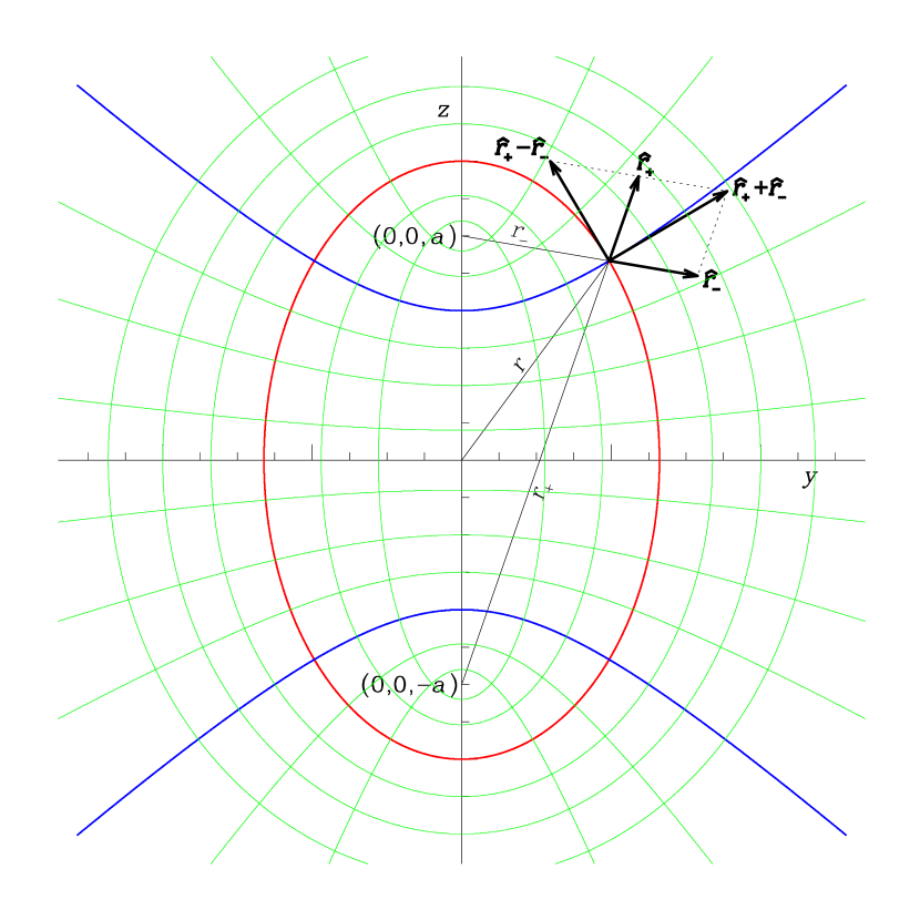
Figure 1: $yz$-plane cross-section of prolate spheroidal coordinate surfaces.

Let us consider the quadratic form on $\mn@boldsymbol{v}$ (cf. Lynden-Bell, 2003),

$$\mathsf{\tilde{Q}}_{a}(\mn@boldsymbol{v})=(\mn@boldsymbol{r_{+}}\mn@boldsymbol{\times}\mn@boldsymbol{v})\mn@boldsymbol{\cdot}(\mn@boldsymbol{r_{-}}\mn@boldsymbol{\times}\mn@boldsymbol{v}),$$ (19a)

where $$\mn@boldsymbol{r_{\pm}}=\mn@boldsymbol{r}\pm a{\hat{\Bbbk\mkern-3.0mu}\mkern 3.0mu}{} \mn@boldsymbol{r_{\pm}}\mn@boldsymbol{\times}\mn@boldsymbol{v}=\mn@boldsymbol{L}\pm a\mn@boldsymbol{\ell} \mn@boldsymbol{\ell}={\hat{\Bbbk\mkern-3.0mu}\mkern 3.0mu}{}\mn@boldsymbol{\times}\mn@boldsymbol{v} \mathsf{\tilde{Q}}_{a}(\mn@boldsymbol{v})=L^{2}-a^{2}\ell^{2} \ell^{2}=\lVert\mn@boldsymbol{\ell}\rVert^{2}=({\hat{\Bbbk\mkern-3.0mu}\mkern 3.0mu}{}\mn@boldsymbol{\cdot}{\hat{\Bbbk\mkern-3.0mu}\mkern 3.0mu}{})(\mn@boldsymbol{v}\mn@boldsymbol{\cdot}\mn@boldsymbol{v})-({\hat{\Bbbk\mkern-3.0mu}\mkern 3.0mu}{}\mn@boldsymbol{\cdot}\mn@boldsymbol{v})^{2}=v^{2}-v_{z}^{2} \mathsf{\tilde{Q}}_{a}(\mn@boldsymbol{v}) \tilde{I}=2(I-a^{2}\mathcal{H}) I \beta=a^{2}>0$$. Then , where , and so . Yet , and thus is the kinetic part of an integral of motion, where is given by equation (7) with a positive constant .

The quadratic form $\mathsf{\tilde{Q}}_{a}(\mn@boldsymbol{v})$ is useful in finding its diagonalizing frame (in which kinetic parts of $I$ and $\tilde{I}$ also diagonalize). First note

$$\mathsf{\tilde{Q}}_{a}(\mn@boldsymbol{v})=\bigl{[}(\mn@boldsymbol{r_{\pm}}\mn@boldsymbol{\times}\mn@boldsymbol{v})\mn@boldsymbol{\times}\mn@boldsymbol{r_{\mp}}\bigr{]}\mn@boldsymbol{\cdot}\mn@boldsymbol{v},$$ (19b)

which further implies $\mathsf{\tilde{Q}}_{a}(\mn@boldsymbol{v})=\mn@boldsymbol{v}\mn@boldsymbol{\cdot}\mbox{\boldmath${\sl K}$}_{a}(\mn@boldsymbol{v})$ with

$$2\mbox{\boldmath${\sl K}$}_{a}(\mn@boldsymbol{v})=(\mn@boldsymbol{r_{+}}\mn@boldsymbol{\times}\mn@boldsymbol{v})\mn@boldsymbol{\times}\mn@boldsymbol{r_{-}}+(\mn@boldsymbol{r_{-}}\mn@boldsymbol{\times}\mn@boldsymbol{v})\mn@boldsymbol{\times}\mn@boldsymbol{r_{+}},$$ (20)

which is a self-adjoint linear function of $\mn@boldsymbol{v}$ (i.e. a symmetric tensor). If $\set{\hat{\mn@boldsymbol{e}}_{1},\hat{\mn@boldsymbol{e}}_{2},\hat{\mn@boldsymbol{e}}_{3}}$ is the set of its orthonormal eigenvectors and $\kappa_{i}$ is the eigenvalue associated with $\hat{\mn@boldsymbol{e}}_{i}$ such that $\mbox{\boldmath${\sl K}$}_{a}(\hat{\mn@boldsymbol{e}}_{i})=\kappa_{i}\hat{\mn@boldsymbol{e}}_{i}$, then $\mbox{\boldmath${\sl K}$}_{a}(\mn@boldsymbol{v})=\sum_{i=1}^{3}\kappa_{i}v_{i}\hat{\mn@boldsymbol{e}}_{i}$ and $\mathsf{\tilde{Q}}_{a}(\mn@boldsymbol{v})=\sum_{i=1}^{3}\kappa_{i}v_{i}^{2}$, where $v_{i}=\hat{\mn@boldsymbol{e}}_{i}\mn@boldsymbol{\cdot}\mn@boldsymbol{v}$ is the velocity component projected on to $\hat{\mn@boldsymbol{e}}_{i}$. In other words, $\mathsf{\tilde{Q}}_{a}$ diagonalizes in the frame consisting of eigenvectors of $\mbox{\boldmath${\sl K}$}_{a}$.

These eigenvectors are found by observing

$$\begin{split}2\mbox{\boldmath${\sl K}$}_{a}(\mn@boldsymbol{r_{\pm}})&=(\mn@boldsymbol{r_{\mp}}\mn@boldsymbol{\times}\mn@boldsymbol{r_{\pm}})\mn@boldsymbol{\times}\mn@boldsymbol{r_{\pm}}=(\mn@boldsymbol{r_{+}}\mn@boldsymbol{\cdot}\mn@boldsymbol{r_{-}})\mn@boldsymbol{r_{\pm}}-r_{\pm}^{2}\mn@boldsymbol{r_{\mp}};\\ 2\mbox{\boldmath${\sl K}$}_{a}({\hat{\mn@boldsymbol{r_{\pm}}\mkern-5.0mu}\mkern 5.0mu}{})&=(\mn@boldsymbol{r_{+}}\mn@boldsymbol{\cdot}\mn@boldsymbol{r_{-}}){\hat{\mn@boldsymbol{r_{\pm}}\mkern-5.0mu}\mkern 5.0mu}{}-r_{+}r_{-}{\hat{\mn@boldsymbol{r_{\mp}}\mkern-5.0mu}\mkern 5.0mu}{},\end{split}$$ (21a)

where $$r_{\pm}=\lVert\mn@boldsymbol{r_{\pm}}\rVert=\sqrt{\mn@boldsymbol{r_{\pm}}\mn@boldsymbol{\cdot}\mn@boldsymbol{r_{\pm}}} {\hat{\mn@boldsymbol{r_{\pm}}\mkern-5.0mu}\mkern 5.0mu}{}=\mn@boldsymbol{r_{\pm}}/r_{\pm}$$ and . Hence,

$$2\mbox{\boldmath${\sl K}$}_{a}({\hat{\mn@boldsymbol{r_{+}}\mkern-5.0mu}\mkern 5.0mu}{}\pm{\hat{\mn@boldsymbol{r_{-}}\mkern-5.0mu}\mkern 5.0mu}{})=\bigl{(}\mn@boldsymbol{r_{+}}\mn@boldsymbol{\cdot}\mn@boldsymbol{r_{-}}\mp r_{+}r_{-})({\hat{\mn@boldsymbol{r_{+}}\mkern-5.0mu}\mkern 5.0mu}{}\pm{\hat{\mn@boldsymbol{r_{-}}\mkern-5.0mu}\mkern 5.0mu}{}),$$ (21b)

that is, $${\hat{\mn@boldsymbol{r_{+}}\mkern-5.0mu}\mkern 5.0mu}{}\pm{\hat{\mn@boldsymbol{r_{-}}\mkern-5.0mu}\mkern 5.0mu}{} \mbox{\boldmath${\sl K}$}_{a} \hat{\mn@boldsymbol{e}}_{\phi} \mbox{\boldmath${\sl K}$}_{a}(\hat{\mn@boldsymbol{e}}_{\phi})=(r^{2}-a^{2})\hat{\mn@boldsymbol{e}}_{\phi}$$ is the two of (orthogonal but not necessarily normalized) eigenvectors of . The remaining eigenvector is , which is, up to signs, the only unit vector orthogonal to the first two. The associated eigenvalue is found by direct calculations, namely, .

It follows that if $v_{\pm}$ is the velocity component in the direction of ${\hat{\mn@boldsymbol{r_{+}}\mkern-5.0mu}\mkern 5.0mu}{}\pm{\hat{\mn@boldsymbol{r_{-}}\mkern-5.0mu}\mkern 5.0mu}{}$, then the diagonalized $\mathsf{\tilde{Q}}_{a}(\mn@boldsymbol{v})$ is given by

$$2\mathsf{\tilde{Q}}_{a}(\mn@boldsymbol{v})=(l-m)\,v_{+}^{2}+(l+m)\,v_{-}^{2}+2lv_{\phi}^{2},$$ (22)

where $m=r_{+}r_{-}$ and $l=\mn@boldsymbol{r_{+}}\mn@boldsymbol{\cdot}\mn@boldsymbol{r_{-}}=r^{2}-a^{2}$.

In order to interpret these eigenvectors geometrically, we note

$$\begin{split}&\mn@boldsymbol{r_{\pm}}=\mn@boldsymbol{r}\pm a\,{\hat{\Bbbk\mkern-3.0mu}\mkern 3.0mu}{}=\rho\hat{\mn@boldsymbol{e}}_{\rho}+(z\pm a)\,{\hat{\Bbbk\mkern-3.0mu}\mkern 3.0mu}{},\quad r_{\pm}^{2}=\rho^{2}+(z\pm a)^{2};\\ &\mn@boldsymbol{\nabla}r_{\pm}^{2}=2\rho\mn@boldsymbol{e}^{\rho}+2(z\pm a)\mn@boldsymbol{e}^{z}=2\mn@boldsymbol{r_{\pm}},\quad\mn@boldsymbol{\nabla}r_{\pm}^{2}=2r_{\pm}(\mn@boldsymbol{\nabla}r_{\pm});\\ &\therefore{\hat{\mn@boldsymbol{r_{\pm}}\mkern-5.0mu}\mkern 5.0mu}{}=\mn@boldsymbol{r_{\pm}}/r_{\pm}=\mn@boldsymbol{\nabla}r_{\pm}.\end{split}$$ (23)

Hence ${\hat{\mn@boldsymbol{r_{+}}\mkern-5.0mu}\mkern 5.0mu}{}\pm{\hat{\mn@boldsymbol{r_{-}}\mkern-5.0mu}\mkern 5.0mu}{}$ is normal to the surface defined by a constant value of $r_{+}\pm r_{-}$, respectively. Since $r_{\pm}=\lVert\mn@boldsymbol{r}\pm a\,{\hat{\Bbbk\mkern-3.0mu}\mkern 3.0mu}{}\rVert$ is the respective distance to the point $z=\mp a$ on the $z$-axis, the constant sum defines a confocal set of prolate spheroids whilst the constant difference does that of circular hyperboloids of two sheets – see Fig. 1. Together with the meridional planes, they constitute a pair-wise orthogonal foliation of the three-dimensional Euclidean space ($\mathbb{R}^{3}$). Any set of monotonic differentiable functions on each leaf in the family then defines an orthogonal coordinate in which $\mathsf{\tilde{Q}}_{a}$ diagonalizes. Within arbitrary scalings, this coordinate system corresponds to the prolate spheroidal coordinate with the foci on $(x,y,z)=(0,0,\pm a)$. An intuitive choice for the meridional coordinate variables is $(\zeta,\eta)=(r_{+}+r_{-},r_{+}-r_{-})$, that is, the sum of and the difference between the distances to two foci. Here $\zeta/2$ and $\eta/2$ are also the semimajor axes of the meridional ellipse and hyperbola, and so each essentially labels the particular coordinate surface. More common choice however is either $(\upsilon,\nu,\phi)$, where $(\zeta,\eta)=(2a\cosh\upsilon,2a\cos\nu)$ (e.g., Kent & de Zeeuw, 1991; Binney, 2012) or $(\lambda,\mu,\phi)$, where $(\zeta^{2},\eta^{2})=[4(\lambda+a^{2}+\alpha),4(\mu+a^{2}+\alpha)]$ with a constant $\alpha$ (e.g., Dejonghe & de Zeeuw, 1988; Sanders, 2012).

The potential admitting the integral $\tilde{I}$ is characterized in the same coordinate system by considering the vector field,

$$2\mbox{\boldmath${\sl K}$}_{a}(\mn@boldsymbol{\nabla}\psi)=-\bigl{[}\mn@boldsymbol{r_{+}}\mn@boldsymbol{\times}(\mn@boldsymbol{r_{-}}\mn@boldsymbol{\times}\mn@boldsymbol{\nabla}\psi)+\mn@boldsymbol{r_{-}}\mn@boldsymbol{\times}(\mn@boldsymbol{r_{+}}\mn@boldsymbol{\times}\mn@boldsymbol{\nabla}\psi)\bigr{]}.$$ (24a)

Since $$\mn@boldsymbol{r_{\pm}}\mn@boldsymbol{\times}\mn@boldsymbol{\nabla}\psi=\hat{\mn@boldsymbol{e}}_{\phi}\bigl{(}\partial_{\theta}\psi\rvert_{r}\pm a\partial_{\rho}\psi\rvert_{z}\bigr{)}$$, we find (cf. eq. 9)

$$\mbox{\boldmath${\sl K}$}_{a}(\mn@boldsymbol{\nabla}\psi)=r\hat{\mn@boldsymbol{e}}_{\theta}\partial_{\theta}\psi\rvert_{r}-a^{2}\hat{\mn@boldsymbol{e}}_{\rho}\partial_{\rho}\psi\rvert_{z}=\mn@boldsymbol{\nabla}(\xi-a^{2}\psi),$$ (24b)

and so $\mbox{\boldmath${\sl K}$}_{a}(\mn@boldsymbol{\nabla}\psi)$ is curl free. For the meridional coordinate $(\zeta,\eta)=(r_{+}+r_{-},r_{+}-r_{-})$, equation (23) indicates that $(\mn@boldsymbol{\nabla}\zeta,\mn@boldsymbol{\nabla}\eta)=({\hat{\mn@boldsymbol{r_{+}}\mkern-5.0mu}\mkern 5.0mu}{}+{\hat{\mn@boldsymbol{r_{-}}\mkern-5.0mu}\mkern 5.0mu}{},{\hat{\mn@boldsymbol{r_{+}}\mkern-5.0mu}\mkern 5.0mu}{}-{\hat{\mn@boldsymbol{r_{-}}\mkern-5.0mu}\mkern 5.0mu}{})$ and $\mn@boldsymbol{\nabla}=({\hat{\mn@boldsymbol{r_{+}}\mkern-5.0mu}\mkern 5.0mu}{}+{\hat{\mn@boldsymbol{r_{-}}\mkern-5.0mu}\mkern 5.0mu}{})\partial_{\zeta}+({\hat{\mn@boldsymbol{r_{+}}\mkern-5.0mu}\mkern 5.0mu}{}-{\hat{\mn@boldsymbol{r_{-}}\mkern-5.0mu}\mkern 5.0mu}{})\partial_{\eta}+\mn@boldsymbol{e}^{\phi}\partial_{\phi}$. Defining $\mathcal{D}_{\pm}=\partial_{\zeta}\pm\partial_{\eta}$ and also assuming $\partial_{\phi}=0$, we then have

$${\hat{\mn@boldsymbol{r_{+}}\mkern-5.0mu}\mkern 5.0mu}{}\mn@boldsymbol{\times}\mn@boldsymbol{\nabla}={\hat{\mn@boldsymbol{r_{+}}\mkern-5.0mu}\mkern 5.0mu}{}\mn@boldsymbol{\times}{\hat{\mn@boldsymbol{r_{-}}\mkern-5.0mu}\mkern 5.0mu}{}\mathcal{D}_{-},\quad{\hat{\mn@boldsymbol{r_{-}}\mkern-5.0mu}\mkern 5.0mu}{}\mn@boldsymbol{\times}\mn@boldsymbol{\nabla}={\hat{\mn@boldsymbol{r_{-}}\mkern-5.0mu}\mkern 5.0mu}{}\mn@boldsymbol{\times}{\hat{\mn@boldsymbol{r_{+}}\mkern-5.0mu}\mkern 5.0mu}{}\mathcal{D}_{+};$$

$$\mn@boldsymbol{r_{\pm}}\mn@boldsymbol{\times}(\mn@boldsymbol{r_{\mp}}\mn@boldsymbol{\times}\mn@boldsymbol{\nabla}\psi)=\mn@boldsymbol{r_{\pm}}\mn@boldsymbol{\times}(\mn@boldsymbol{r_{\mp}}\mn@boldsymbol{\times}{\hat{\mn@boldsymbol{r_{\pm}}\mkern-5.0mu}\mkern 5.0mu}{})\mathcal{D}_{\pm}(\psi)=(m{\hat{\mn@boldsymbol{r_{\mp}}\mkern-5.0mu}\mkern 5.0mu}{}-l{\hat{\mn@boldsymbol{r_{\pm}}\mkern-5.0mu}\mkern 5.0mu}{})\mathcal{D}_{\pm}(\psi);$$

$$\mbox{\boldmath${\sl K}$}_{a}(\mn@boldsymbol{\nabla}\psi)=\bigl{[}{\hat{\mn@boldsymbol{r_{+}}\mkern-5.0mu}\mkern 5.0mu}{}\,(l\mathcal{D}_{+}-m\mathcal{D}_{-})+{\hat{\mn@boldsymbol{r_{-}}\mkern-5.0mu}\mkern 5.0mu}{}\,(l\mathcal{D}_{-}-m\mathcal{D}_{+})\bigr{]}\,\psi,$$ (25)

where again $m=r_{+}r_{-}$ and $l=\mn@boldsymbol{r_{+}}\mn@boldsymbol{\cdot}\mn@boldsymbol{r_{-}}=r^{2}-a^{2}$. Consequently

$$\mn@boldsymbol{\nabla}\mn@boldsymbol{\times}\mbox{\boldmath${\sl K}$}_{a}(\mn@boldsymbol{\nabla}\psi)=2a\rho\hat{\mn@boldsymbol{e}}_{\phi}\bigl{(}\mathcal{D}_{-}^{2}-\mathcal{D}_{+}^{2}\bigr{)}\,(m\psi),$$ (26)

provided that $\partial_{\zeta}\partial_{\eta}=\partial_{\eta}\partial_{\zeta}$. Calculations ease using $\mathcal{D}_{\pm}(r_{\pm})=1$ and $\mathcal{D}_{\mp}(r_{\pm})=0$, which follows $2r_{\pm}=\zeta\pm\eta$. In addition, $\mathcal{D}_{\pm}(l)=r_{\pm}$ from $\zeta^{2}+\eta^{2}=2(r_{+}^{2}+r_{-}^{2})=4(r^{2}+a^{2})$ and so $l=(r_{+}^{2}+r_{-}^{2})/2-2a^{2}$. Thus $\mn@boldsymbol{\nabla}\mn@boldsymbol{\times}\mbox{\boldmath${\sl K}$}_{a}(\mn@boldsymbol{\nabla}\psi)=0$ is equivalent to

$$\bigl{(}\mathcal{D}_{+}^{2}-\mathcal{D}_{-}^{2}\bigr{)}\,(m\psi)=4\frac{\partial^{2}(m\psi)}{\partial\zeta\partial\eta}=0\quad\Rightarrow\ \psi=\frac{f(\zeta)+g(\eta)}{m},$$ (27a)

where $$f g$$ and are arbitrary functions of respective argument and

$$\begin{split}m&=r_{+}r_{-}=(\zeta^{2}-\eta^{2})/4=\lambda-\mu\\ &=a^{2}(\cosh^{2}\upsilon-\cos^{2}\nu)=a^{2}(\sinh^{2}\upsilon+\sin^{2}\nu)\end{split}$$ (27b)

with $(\upsilon,\nu)$ and $(\lambda,\mu)$ as defined earlier. Hence, an axially symmetric potential with the ratio in equation (7) being a positive constant $\beta=a^{2}>0$ is the Stäckel potential (e.g., Lynden-Bell, 1962; de Zeeuw, 1985c; Evans & Lynden-Bell, 1989) separable in the prolate spheroidal coordinate with the foci located on $z=\pm a$ on the symmetry axis.

The opposite implication, that any Stäckel potential separable in a prolate spheroidal coordinate results in a positive constant for equation (7), is trivial from its transformations back to the cylindrical and spherical polar coordinates. For instance, with the coordinate transform $(\lambda,\mu)\to(\rho^{2},z^{2})$ (see e.g., Lynden-Bell, 1962),

$$\rho^{2}=\frac{(\lambda+\alpha)(\mu+\alpha)}{\alpha-\beta},\quad z^{2}=\frac{(\lambda+\beta)(\mu+\beta)}{\beta-\alpha},$$ (28a)

the differential equation in equation (27) transforms to

$$\frac{\partial^{2}\bigl{[}(\lambda-\mu)\psi\bigr{]}}{\partial\lambda\partial\mu}=\frac{\partial\psi}{\partial\mu}-\frac{\partial\psi}{\partial\lambda}+(\lambda-\mu)\frac{\partial^{2}\psi}{\partial\lambda\partial\mu}=\frac{\lambda-\mu}{4(\beta-\alpha)}\\ \times\Biggl{[}\frac{1}{z^{3}}\frac{\partial}{\partial z}\biggl{(}z^{3}\frac{\partial\psi}{\partial z}\biggr{)}-\frac{1}{\rho^{3}}\frac{\partial}{\partial\rho}\biggl{(}\rho^{3}\frac{\partial\psi}{\partial\rho}\biggr{)}+\frac{\rho^{2}-z^{2}+\beta-\alpha}{\rho z}\frac{\partial^{2}\psi}{\partial\rho\partial z}\Biggr{]}$$ (28b)

in the cylindrical polar coordinate. We furthermore find that

$$\frac{1}{\rho^{3}}\frac{\partial}{\partial\rho}\biggl{(}\rho^{3}\frac{\partial\psi}{\partial\rho}\biggr{)}-\frac{1}{z^{3}}\frac{\partial}{\partial z}\biggl{(}z^{3}\frac{\partial\psi}{\partial z}\biggr{)}-\frac{\rho^{2}-z^{2}}{\rho z}\frac{\partial^{2}\psi}{\partial\rho\partial z}\\ =\biggl{(}\frac{1}{\rho^{k}z^{3-k}}\frac{\partial}{\partial\rho}+\frac{1}{\rho^{1+k}z^{2-k}}\frac{\partial}{\partial z}\biggr{)}\,\biggl{(}\rho^{k}z^{3-k}\frac{\partial\psi}{\partial\rho}-\rho^{1+k}z^{2-k}\frac{\partial\psi}{\partial z}\biggr{)},$$ (29a)

where $$k \partial_{\rho}=\sin\theta\,\partial_{r}+r^{-1}\!\cos\theta\,\partial_{\theta} \partial_{z}=\cos\theta\,\partial_{r}-r^{-1}\!\sin\theta\,\partial_{\theta}$$ is any fixed real number. However, the transformation to the spherical polar coordinate and indicates that

$$\begin{split}\frac{1}{\rho^{k}z^{3-k}}&\frac{\partial}{\partial\rho}+\frac{1}{\rho^{1+k}z^{2-k}}\frac{\partial}{\partial z}=\frac{1}{r^{3}\sin^{1+k}\!\theta\cos^{3-k}\!\theta}\frac{\partial}{\partial r},\\ \rho^{k}z^{3-k}&\frac{\partial}{\partial\rho}-\rho^{1+k}z^{2-k}\frac{\partial}{\partial z}=r^{2}\sin^{k}\!\theta\cos^{2-k}\!\theta\frac{\partial}{\partial\theta}.\end{split}$$ (29b)

So the Stäckel potential separable in a prolate spheroidal coordinate satisfies the differential equation (cf. Sanders, 2012, eq. 9)

$$\frac{\partial^{2}\bigl{[}(\lambda-\mu)\psi\bigr{]}}{\partial\lambda\partial\mu}=\frac{\lambda-\mu}{4\rho z\delta}\Biggl{[}\delta\frac{\partial^{2}\psi}{\partial\rho\partial z}-\frac{1}{r}\frac{\partial}{\partial r}\biggl{(}r^{2}\frac{\partial\psi}{\partial\theta}\biggr{)}\Biggr{]}=0,$$ (30)

where $\delta=\beta-\alpha$, which is a positive constant.

4.2 Oblate spheroidal coordinates

If $\beta=-a^{2}<0$ in equation (7) is a negative constant, the integral of motion $I$ in equation (8) may be written down to be $2I=\mathsf{\bar{Q}}_{a}(\mn@boldsymbol{v})+a^{2}(\hat{\mn@boldsymbol{e}}_{\phi}\mn@boldsymbol{\cdot}\mn@boldsymbol{v})^{2}+\xi(\mn@boldsymbol{r})$ introducing another quadratic form:

$$\mathsf{\bar{Q}}_{a}(\mn@boldsymbol{v})=(\mn@boldsymbol{q_{+}}\mn@boldsymbol{\times}\mn@boldsymbol{v})\mn@boldsymbol{\cdot}(\mn@boldsymbol{q_{-}}\mn@boldsymbol{\times}\mn@boldsymbol{v}),$$ (31)

where $\mn@boldsymbol{q_{\pm}}=\mn@boldsymbol{r}\pm a\hat{\mn@boldsymbol{e}}_{\rho}$. Essentially verbatim calculations as in the preceding section establish that $\mathsf{\bar{Q}}_{a}(\mn@boldsymbol{v})$ diagonalizes in the frame defined by $\set{{\hat{\mn@boldsymbol{q_{+}}\mkern-6.0mu}\mkern 6.0mu}{}\pm{\hat{\mn@boldsymbol{q_{-}}\mkern-6.0mu}\mkern 6.0mu}{},\hat{\mn@boldsymbol{e}}_{\phi}}$, where ${\hat{\mn@boldsymbol{q_{\pm}}\mkern-6.0mu}\mkern 6.0mu}{}=\mn@boldsymbol{q_{\pm}}/\lVert\mn@boldsymbol{q_{\pm}}\rVert$. So does the kinetic part of $I$ since $v_{\phi}^{2}$ trivially diagonalizes in the same frame.

The meridional cross-section of the coordinate surfaces defined by this frame set is basically the same as before except for the $R$- and $z$-axes switched (see again Fig. 1). That is to say, the symmetry axis now lies along the minor axis of the ellipse. These result in the coordinate surfaces being the confocal oblate spheroids and circular hyperboloids of one sheet whilst the resulting coordinate system is identified with the oblate spheroidal coordinate with the meridional foci on the mid-plane point $R=(\pm)a$. Note that the derivation of equation (27) in the preceding section considers only the two-dimensional coordinates restricted to the meridional plane. Therefore, the same calculations (with the $\mn@boldsymbol{r_{\pm}}\to\mn@boldsymbol{q_{\pm}}$ replacement) can be used to show that the axially symmetric potential that results in a negative constant $\beta=-a^{2}$ in equation (7) is also the Stäckel potential but separable in an oblate spheroidal coordinate.

4.3 Degenerate cases

If $\partial_{r}\partial_{\theta}(r^{2}\psi)=0$ or $\partial_{\rho}\partial_{z}\psi=0$, equation (7) is also considered constant. In fact, this indicates that the axially symmetric potential is of the separable form in the spherical or cylindrical polar coordinate,

$$\partial_{r}\partial_{\theta}(r^{2}\psi)=0 \Longleftrightarrow \psi =f(r)+r^{-2}g(\theta);$$ (32)

$$\partial_{\rho}\partial_{z}\psi=0 \Longleftrightarrow \psi =f(\rho)+g(z).$$ (33)

Given arbitrary functions $f$ and $g$, the third integrals besides the energy, $\mathcal{H}$, and the axial angular momentum component, $L_{z}$, are, $\frac{1}{2}L^{2}+g(\theta)$ and $\frac{1}{2}v_{z}^{2}+g(z)$, respectively. These are consistent with equations (8) and (9), either setting $\beta=0$ or considering $\lim_{\beta\rightarrow\infty}\beta^{-1}I$. With equation (33), the $z$-motion decouples and the third integral is basically the corresponding one-dimensional energy. The third integral for equation (32) on the other hand is essentially the Hamiltonian of the angular motion projected along the radial direction on to the unit sphere. If $g=0$ in either case, the quadratic integral is simply the square of momentum, namely $\mn@boldsymbol{L}$ or $v_{z}$. Note that equation (32) then reduces to spherically symmetric potentials and is actually superintegrable since $\mn@boldsymbol{L}$ counts as two additional integrals, $(L_{x},L_{y})$.

If both $\partial_{r}\partial_{\theta}(r^{2}\psi)=0$ and $\partial_{\rho}\partial_{z}\psi=0$, the potential is completely specified. That is to say, the general solution is then given by

$$\psi=k_{0}r^{2}+k_{1}\rho^{-2}+k_{2}z^{-2}+k_{3},$$ (34)

which involves constants but not arbitrary functions. The particular example includes the harmonic potential $(\psi=k_{0}r^{2})$. This potential is separable in both the spherical and cylindrical polar coordinates as well as any prolate or oblate spheroidal coordinates with arbitrary parameter $a$ (formally $\beta=0/0$ is an indeterminate constant). Dynamics in the potential of equation (34) is not only superintegrable (i.e. the orbit projected on to the meridional plane becomes a closed curve) but also completely soluble in a closed form using only elementary functions. If $k_{1}=0$, the potential is further separable in the Cartesian coordinate and so maximally superintegrable (i.e. the orbits are thus truly periodic).

5 Separability with an unspecified origin

The discussion so far has implicitly assumed that the coordinate origin of the frame about which the angular momentum is defined is known a priori. Relaxing this restriction is equivalent to allowing the coordinate origin to be an arbitrary point on the symmetry axis. The angular momentum with respect to the point $z=\alpha$ on the symmetry axis is given by $\mn@boldsymbol{L}_{\alpha}=(\mn@boldsymbol{r}-\alpha{\hat{\Bbbk\mkern-3.0mu}\mkern 3.0mu}{})\mn@boldsymbol{\times}\mn@boldsymbol{v}=\mn@boldsymbol{L}-\alpha\mn@boldsymbol{\ell}$, where $\mn@boldsymbol{L}$ is the angular momentum with respect to $z=0$ and $\mn@boldsymbol{\ell}={\hat{\Bbbk\mkern-3.0mu}\mkern 3.0mu}{}\mn@boldsymbol{\times}\mn@boldsymbol{v}$. Then $L_{\alpha}^{2}=L^{2}-2\alpha\omega+\alpha^{2}\ell^{2}$, where $\omega=\mn@boldsymbol{\ell}\mn@boldsymbol{\cdot}\mn@boldsymbol{L}=(\mn@boldsymbol{v}\mn@boldsymbol{\times}\mn@boldsymbol{L})\mn@boldsymbol{\cdot}{\hat{\Bbbk\mkern-3.0mu}\mkern 3.0mu}{}$ and $\ell^{2}=v^{2}-v_{z}^{2}$. From equation (1), $\dot{\mn@boldsymbol{\ell}}=-{\hat{\Bbbk\mkern-3.0mu}\mkern 3.0mu}{}\mn@boldsymbol{\times}\mn@boldsymbol{\nabla}\psi$ and so

$$\tfrac{1}{2}D_{t}\ell^{2}=\mn@boldsymbol{\ell}\mn@boldsymbol{\cdot}\dot{\mn@boldsymbol{\ell}}=(\mn@boldsymbol{v}\mn@boldsymbol{\times}{\hat{\Bbbk\mkern-3.0mu}\mkern 3.0mu}{})\mn@boldsymbol{\cdot}({\hat{\Bbbk\mkern-3.0mu}\mkern 3.0mu}{}\mn@boldsymbol{\times}\mn@boldsymbol{\nabla}\psi)=\mn@boldsymbol{v}\mn@boldsymbol{\cdot}\bigl{[}{\hat{\Bbbk\mkern-3.0mu}\mkern 3.0mu}{}\mn@boldsymbol{\times}({\hat{\Bbbk\mkern-3.0mu}\mkern 3.0mu}{}\mn@boldsymbol{\times}\mn@boldsymbol{\nabla}\psi)\bigr{]},$$ (35a)

$$\begin{split}\dot{\omega}=\dot{\mn@boldsymbol{\ell}}\mn@boldsymbol{\cdot}\mn@boldsymbol{L}+\mn@boldsymbol{\ell}\mn@boldsymbol{\cdot}\dot{\mn@boldsymbol{L}}&=(\mn@boldsymbol{v}\mn@boldsymbol{\times}\mn@boldsymbol{r})\mn@boldsymbol{\cdot}({\hat{\Bbbk\mkern-3.0mu}\mkern 3.0mu}{}\mn@boldsymbol{\times}\mn@boldsymbol{\nabla}\psi)+(\mn@boldsymbol{v}\mn@boldsymbol{\times}{\hat{\Bbbk\mkern-3.0mu}\mkern 3.0mu}{})\mn@boldsymbol{\cdot}(\mn@boldsymbol{r}\mn@boldsymbol{\times}\mn@boldsymbol{\nabla}\psi)\\ &=\mn@boldsymbol{v}\mn@boldsymbol{\cdot}\bigl{[}\mn@boldsymbol{r}\mn@boldsymbol{\times}({\hat{\Bbbk\mkern-3.0mu}\mkern 3.0mu}{}\mn@boldsymbol{\times}\mn@boldsymbol{\nabla}\psi)+{\hat{\Bbbk\mkern-3.0mu}\mkern 3.0mu}{}\mn@boldsymbol{\times}(\mn@boldsymbol{r}\mn@boldsymbol{\times}\mn@boldsymbol{\nabla}\psi)\bigr{]}.\end{split}$$ (35b)

Hence, $D_{t}L_{\alpha}^{2}=-2\mn@boldsymbol{v}\mn@boldsymbol{\cdot}(\mn@boldsymbol{s}-\alpha\mn@boldsymbol{h}+\alpha^{2}\mn@boldsymbol{k})$, where $\mn@boldsymbol{s}$ is as in equation (3),

$$\mn@boldsymbol{s}=-\mn@boldsymbol{r}\mn@boldsymbol{\times}(\mn@boldsymbol{r}\mn@boldsymbol{\times}\mn@boldsymbol{\nabla}\psi)=r^{2}(\mn@boldsymbol{\nabla}\psi-\mn@boldsymbol{e}^{r}\partial_{r}\psi),$$ (36a)

and also introduced are the vector fields

$$\begin{split}\mn@boldsymbol{h}&=-\bigl{[}\mn@boldsymbol{r}\mn@boldsymbol{\times}({\hat{\Bbbk\mkern-3.0mu}\mkern 3.0mu}{}\mn@boldsymbol{\times}\mn@boldsymbol{\nabla}\psi)+{\hat{\Bbbk\mkern-3.0mu}\mkern 3.0mu}{}\mn@boldsymbol{\times}(\mn@boldsymbol{r}\mn@boldsymbol{\times}\mn@boldsymbol{\nabla}\psi)\bigr{]},\\ \mn@boldsymbol{k}&=-{\hat{\Bbbk\mkern-3.0mu}\mkern 3.0mu}{}\mn@boldsymbol{\times}({\hat{\Bbbk\mkern-3.0mu}\mkern 3.0mu}{}\mn@boldsymbol{\times}\mn@boldsymbol{\nabla}\psi)=\mn@boldsymbol{\nabla}\psi-{\hat{\Bbbk\mkern-3.0mu}\mkern 3.0mu}{}\,\partial_{z}\psi.\end{split}$$ (36b)

Following a similar argument as in Sect. 2, we conclude that, if there exist real constants $a,b,c$ such that (NB: $\mn@boldsymbol{\nabla}\mn@boldsymbol{\times}\mn@boldsymbol{\nabla}\psi=0$)

$$a\,\mn@boldsymbol{\nabla}\mn@boldsymbol{\times}\mn@boldsymbol{s}-b\,\mn@boldsymbol{\nabla}\mn@boldsymbol{\times}\mn@boldsymbol{h}-c\,\mn@boldsymbol{\nabla}\mn@boldsymbol{\times}\mn@boldsymbol{k}=0\qquad(a^{2}+b^{2}+c^{2}\neq 0),$$ (37)

then there exists the scalar function $\xi$ which is the solution of

$$\mn@boldsymbol{\nabla}\xi=a\mn@boldsymbol{s}-b\mn@boldsymbol{h}-c\mn@boldsymbol{k},$$ (38)

and therefore the potential admits an integral of motion,

$$2I=aL^{2}-2b\omega-c\ell^{2}+2\xi,$$ (39a)

or equivalently

$$2\tilde{I}=2(I+c\mathcal{H})=aL^{2}-2b\omega+cv_{z}^{2}+2(\xi+c\psi).$$ (39b)

If $a\neq 0$, we can find an integral with the kinetic part given by $2Q_{a}=L_{\alpha}^{2}+\beta v_{z}^{2}$, namely $a^{-1}I+\beta\mathcal{H}=a^{-1}\tilde{I}+\alpha^{2}\mathcal{H}=Q_{a}+a^{-1}\xi+\beta\psi$, where $\alpha=b/a$ and $\beta=\alpha^{2}+c/a$. This indicates that, depending on $\beta$, the potential is separable in the prolate spheroidal ($\beta>0$), the spherical polar ($\beta=0$) or the oblate spheroidal ($\beta<0$) coordinate with the origin displaced to $z=\alpha$ on the symmetry axis.

For an axisymmetric system ($\partial_{\phi}=0$),

$$\begin{split}\mn@boldsymbol{s}&=\mn@boldsymbol{e}^{\theta}\partial_{\theta}(r^{2}\psi),&\mn@boldsymbol{\nabla}\mn@boldsymbol{\times}\mn@boldsymbol{s}&=\hat{\mn@boldsymbol{e}}_{\phi}\mathfrak{s},&\mathfrak{s}&=r^{-1}\partial_{r}\partial_{\theta}(r^{2}\psi);\\ \mn@boldsymbol{k}&=\mn@boldsymbol{e}^{\rho}\partial_{\rho}\psi,&\mn@boldsymbol{\nabla}\mn@boldsymbol{\times}\mn@boldsymbol{k}&=\hat{\mn@boldsymbol{e}}_{\phi}\mathfrak{k},&\mathfrak{k}&=\partial_{z}\partial_{\rho}\psi.\end{split}$$ (40)

However, the vector field $\mn@boldsymbol{\nabla}\mn@boldsymbol{\times}\mn@boldsymbol{h}=\hat{\mn@boldsymbol{e}}_{\phi}\mathfrak{h}$, whilst still parallel to $\hat{\mn@boldsymbol{e}}_{\phi}$, results in rather complicated expressions, ($\psi_{r}=\partial_{r}\psi$ & $\psi_{\theta}=\partial_{\theta}\psi$)

$$\mathfrak{h}=\rho(\partial_{\rho}^{2}-\partial_{z}^{2})\psi+3\partial_{\rho}\psi+2z\partial_{z}\partial_{\rho}\psi\\ =r\sin\theta\,\partial_{r}^{2}\psi+2(\sin\theta+\cos\theta\,\partial_{\theta})\psi_{r}+r^{-1}(\cos\theta-\sin\theta\,\partial_{\theta})\psi_{\theta}\\ =\frac{\sin\theta}{r}\frac{\partial(r^{2}\psi_{r})}{\partial r}-\frac{1}{r\sin^{2}\!\theta}\frac{\partial(\psi_{\theta}\sin^{3}\!\theta)}{\partial\theta}+\frac{2\cos\theta}{r^{2}}\frac{\partial^{2}(r^{2}\psi)}{\partial r\partial\theta}$$ (41)

in the cylindrical and spherical polar coordinates (NB: the simplest coordinate expression is obtained with the rotational parabolic coordinate as shall be shown). The condition in equation (37) for an axisymmetric potential is then equivalent to three functions $\mathfrak{s,h,k}$ being linearly dependent. Here the linear dependence is considered within the infinite-dimensional functional space, not in the sense of the vector field on the three-dimensional configuration space. The algebraic necessary (but not sufficient) condition is for all the generalized Wronskians $\set{W(\mathfrak{s},\mathfrak{h},\mathfrak{k})}$ to identically vanish and also

$$\begin{vmatrix}\mathfrak{s}&\mathfrak{h}&\mathfrak{k}\\ \partial_{1}\mathfrak{s}&\partial_{1}\mathfrak{h}&\partial_{1}\mathfrak{k}\\ \partial_{2}\mathfrak{s}&\partial_{2}\mathfrak{h}&\partial_{2}\mathfrak{k}\end{vmatrix}=0,$$ (42)

where $\partial_{i}=\partial/\partial x_{i}$ and $(x_{1},x_{2})$ represents any coordinate on the meridional plane – e.g., $(\rho,z)$ or $(r,\theta)$.

5.1 Rotational parabolic coordinates

If $\mathfrak{h}/\mathfrak{k}=2\gamma$ is constant, then $0\cdot\mathfrak{s}+1\cdot\mathfrak{h}-2\gamma\mathfrak{k}=0$ and so

$$I=\omega-\gamma\ell^{2}+\xi\qquad(\mn@boldsymbol{\nabla}\xi=\mn@boldsymbol{h}-2\gamma\mn@boldsymbol{k})$$ (43)

is an integral of motion. Here the kinetic part is given by

$$\omega-\gamma\ell^{2}=\mn@boldsymbol{\ell}\mn@boldsymbol{\cdot}(\mn@boldsymbol{L}-\gamma\mn@boldsymbol{\ell})=\mn@boldsymbol{\ell}\mn@boldsymbol{\cdot}(\mn@boldsymbol{r}_{\gamma}\mn@boldsymbol{\times}\mn@boldsymbol{v})=\mn@boldsymbol{v}\mn@boldsymbol{\cdot}\mbox{\boldmath${\sl P}$}_{\gamma}(\mn@boldsymbol{v}),$$ (44)

where $\mn@boldsymbol{r}_{\gamma}=\mn@boldsymbol{r}-\gamma{\hat{\Bbbk\mkern-3.0mu}\mkern 3.0mu}{}$ and

$$2\mbox{\boldmath${\sl P}$}_{\gamma}(\mn@boldsymbol{v})=-\bigl{[}\mn@boldsymbol{r}_{\gamma}\mn@boldsymbol{\times}({\hat{\Bbbk\mkern-3.0mu}\mkern 3.0mu}{}\mn@boldsymbol{\times}\mn@boldsymbol{v})+{\hat{\Bbbk\mkern-3.0mu}\mkern 3.0mu}{}\mn@boldsymbol{\times}(\mn@boldsymbol{r}_{\gamma}\mn@boldsymbol{\times}\mn@boldsymbol{v})\bigr{]}$$ (45)

is a self-adjoint linear function of $\mn@boldsymbol{v}$. Next we find

$$\begin{split}2\mbox{\boldmath${\sl P}$}_{\gamma}&(\mn@boldsymbol{r}_{\gamma})=-\mn@boldsymbol{r}_{\gamma}\mn@boldsymbol{\times}({\hat{\Bbbk\mkern-3.0mu}\mkern 3.0mu}{}\mn@boldsymbol{\times}\mn@boldsymbol{r}_{\gamma})=(\mn@boldsymbol{r}_{\gamma}\mn@boldsymbol{\cdot}{\hat{\Bbbk\mkern-3.0mu}\mkern 3.0mu}{})\,\mn@boldsymbol{r}_{\gamma}-r_{\gamma}^{2}\,{\hat{\Bbbk\mkern-3.0mu}\mkern 3.0mu}{},\\ 2\mbox{\boldmath${\sl P}$}_{\gamma}&({\hat{\Bbbk\mkern-3.0mu}\mkern 3.0mu}{})=-{\hat{\Bbbk\mkern-3.0mu}\mkern 3.0mu}{}\mn@boldsymbol{\times}(\mn@boldsymbol{r}_{\gamma}\mn@boldsymbol{\times}{\hat{\Bbbk\mkern-3.0mu}\mkern 3.0mu}{})=(\mn@boldsymbol{r}_{\gamma}\mn@boldsymbol{\cdot}{\hat{\Bbbk\mkern-3.0mu}\mkern 3.0mu}{})\,{\hat{\Bbbk\mkern-3.0mu}\mkern 3.0mu}{}-\mn@boldsymbol{r}_{\gamma},\end{split}$$ (46a)

where $$r_{\gamma}=\lVert\mn@boldsymbol{r}_{\gamma}\rVert (x,y,z)=(0,0,\gamma)$$ is the distance to . Then

$$\begin{split}2\mbox{\boldmath${\sl P}$}_{\gamma}({\hat{\mn@boldsymbol{r}\mkern 2.0mu}\mkern-2.0mu}{}_{\gamma}\pm{\hat{\Bbbk\mkern-3.0mu}\mkern 3.0mu}{})&=(\mn@boldsymbol{r}_{\gamma}\mn@boldsymbol{\cdot}{\hat{\Bbbk\mkern-3.0mu}\mkern 3.0mu}{})\,{\hat{\mn@boldsymbol{r}\mkern 2.0mu}\mkern-2.0mu}{}_{\gamma}-r_{\gamma}\,{\hat{\Bbbk\mkern-3.0mu}\mkern 3.0mu}{}\pm[(\mn@boldsymbol{r}_{\gamma}\mn@boldsymbol{\cdot}{\hat{\Bbbk\mkern-3.0mu}\mkern 3.0mu}{})\,{\hat{\Bbbk\mkern-3.0mu}\mkern 3.0mu}{}-r_{\gamma}\,{\hat{\mn@boldsymbol{r}\mkern 2.0mu}\mkern-2.0mu}{}_{\gamma}]\\ &=(\mn@boldsymbol{r}_{\gamma}\mn@boldsymbol{\cdot}{\hat{\Bbbk\mkern-3.0mu}\mkern 3.0mu}{}\mp r_{\gamma})({\hat{\mn@boldsymbol{r}\mkern 2.0mu}\mkern-2.0mu}{}_{\gamma}\pm{\hat{\Bbbk\mkern-3.0mu}\mkern 3.0mu}{}),\end{split}$$ (46b)

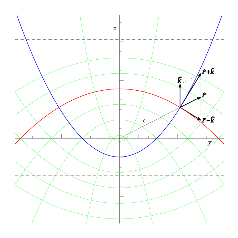
Figure 2: $yz$-plane cross-section of rotational parabolic coordinate surfaces.

where ${\hat{\mn@boldsymbol{r}\mkern 2.0mu}\mkern-2.0mu}{}_{\gamma}=\mn@boldsymbol{r}_{\gamma}/r_{\gamma}$. That is, ${\hat{\mn@boldsymbol{r}\mkern 2.0mu}\mkern-2.0mu}{}_{\gamma}\pm{\hat{\Bbbk\mkern-3.0mu}\mkern 3.0mu}{}$ is the two of eigenvectors of $\mbox{\boldmath${\sl P}$}_{\gamma}$. Here we note ${\hat{\mn@boldsymbol{r}\mkern 2.0mu}\mkern-2.0mu}{}_{\gamma}=\mn@boldsymbol{\nabla}r_{\gamma}$ (cf. eq. 23) whilst $\mn@boldsymbol{\nabla}z={\hat{\Bbbk\mkern-3.0mu}\mkern 3.0mu}{}$. Hence, two eigenvectors are, respectively, normal to the surfaces defined by constant values of $c_{\pm}=r_{\gamma}\pm z>0$. The geometry of conic sections indicates that the meridional cross-sections of these surfaces are confocal parabolae with the focus at $z=\gamma$ on the symmetry axis (which is also the axis of symmetry of all parabolae) and the directrix given by the horizontal line of $z=\pm c_{\pm}$ (see Fig. 2). These eigenvectors thus define a pair of orthogonal foliations consisting of the set of paraboloids of revolution. They, together with the meridional planes, constitute the complete set of coordinate surfaces of the rotational parabolic (or circular paraboloidal) coordinate with the origin at $(x,y,z)=(0,0,\gamma)$. The standard choice for the scaling functions of the coordinate variables is given by $(\sigma,\tau,\phi)$, where $\sigma^{2}=r_{\gamma}+z_{\gamma}$ and $\tau^{2}=r_{\gamma}-z_{\gamma}$ with $z_{\gamma}=z-\gamma$ and $r_{\gamma}^{2}=\rho^{2}+z_{\gamma}^{2}$. The inverse transformation is then $\rho=\sigma\tau$ and $2z_{\gamma}=\sigma^{2}-\tau^{2}$ (and $2r_{\gamma}=\sigma^{2}+\tau^{2}$). However, alternative choices of coordinate variables such that $(\zeta,\eta)=(\sigma^{2},\tau^{2})$ (e.g., Landau & Lifshitz, 1976; Sridhar & Touma, 1997, who used $\eta=-\tau^{2}$) are not uncommon.

The condition $\mathfrak{h}/\mathfrak{k}=2\gamma$ may be expressed in the parabolic coordinate via explicit coordinate transformations, but utilizing the tensor $\mbox{\boldmath${\sl P}$}_{\gamma}$ simplifies calculations. First we have $2\mbox{\boldmath${\sl P}$}_{\gamma}(\mn@boldsymbol{\nabla}\psi)=\mn@boldsymbol{h}-2\gamma\mn@boldsymbol{k}$, and so $2\mn@boldsymbol{\nabla}\mn@boldsymbol{\times}\mbox{\boldmath${\sl P}$}_{\gamma}(\mn@boldsymbol{\nabla}\psi)=\hat{\mn@boldsymbol{e}}_{\phi}(\mathfrak{h}-2\gamma\mathfrak{k})$. Hence, $\mathfrak{h}=2\gamma\mathfrak{k}$ is equivalent to $\mbox{\boldmath${\sl P}$}_{\gamma}(\mn@boldsymbol{\nabla}\psi)$ being curl free. Equation (46a) together with $\mn@boldsymbol{\nabla}={\hat{\mn@boldsymbol{r}\mkern 2.0mu}\mkern-2.0mu}{}_{\gamma}\partial_{r_{\gamma}}+{\hat{\Bbbk\mkern-3.0mu}\mkern 3.0mu}{}\partial_{z_{\gamma}}+\mn@boldsymbol{e}^{\phi}\partial_{\phi}$ then indicates (NB: $\mn@boldsymbol{r}_{\gamma}\mn@boldsymbol{\cdot}{\hat{\Bbbk\mkern-3.0mu}\mkern 3.0mu}{}=z_{\gamma}$)

$$\begin{split}2\mbox{\boldmath${\sl P}$}_{\gamma}(\mn@boldsymbol{\nabla}\psi)&=(z_{\gamma}{\hat{\mn@boldsymbol{r}\mkern 2.0mu}\mkern-2.0mu}{}_{\gamma}-r_{\gamma}{\hat{\Bbbk\mkern-3.0mu}\mkern 3.0mu}{})\partial_{r_{\gamma}}\psi+(z_{\gamma}{\hat{\Bbbk\mkern-3.0mu}\mkern 3.0mu}{}-\mn@boldsymbol{r}_{\gamma})\partial_{z_{\gamma}}\psi\\ &={\hat{\mn@boldsymbol{r}\mkern 2.0mu}\mkern-2.0mu}{}_{\gamma}(z_{\gamma}\partial_{r_{\gamma}}-r_{\gamma}\partial_{z_{\gamma}})\psi-{\hat{\Bbbk\mkern-3.0mu}\mkern 3.0mu}{}\,(r_{\gamma}\partial_{r_{\gamma}}-z_{\gamma}\partial_{z_{\gamma}})\psi.\end{split}$$ (47a)

Next using the identity $$\mn@boldsymbol{\nabla}\mn@boldsymbol{\times}(a\mn@boldsymbol{v})=(\mn@boldsymbol{\nabla}a)\mn@boldsymbol{\times}\mn@boldsymbol{v}+a(\mn@boldsymbol{\nabla}\mn@boldsymbol{\times}\mn@boldsymbol{v}$$),

$$\begin{split}2\mn@boldsymbol{\nabla}\mn@boldsymbol{\times}&\mbox{\boldmath${\sl P}$}_{\gamma}(\mn@boldsymbol{\nabla}\psi)\\ &={\hat{\Bbbk\mkern-3.0mu}\mkern 3.0mu}{}\mn@boldsymbol{\times}{\hat{\mn@boldsymbol{r}\mkern 2.0mu}\mkern-2.0mu}{}_{\gamma}[\partial_{z_{\gamma}}(z_{\gamma}\partial_{r_{\gamma}}-r_{\gamma}\partial_{z_{\gamma}})+\partial_{r_{\gamma}}(r_{\gamma}\partial_{r_{\gamma}}-z_{\gamma}\partial_{z_{\gamma}})]\psi\\ &=r_{\gamma}^{-1}\rho\hat{\mn@boldsymbol{e}}_{\phi}\,(\partial_{r_{\gamma}}^{2}-\partial_{z_{\gamma}}^{2})(r_{\gamma}\psi)=r_{\gamma}^{-1}\hat{\mn@boldsymbol{e}}_{\phi}\,\partial_{\sigma}\partial_{\tau}(r_{\gamma}\psi),\end{split}$$ (47b)

where $\partial_{\sigma}$ and $\partial_{\tau}$ are the coordinate partial derivative with respect to $(\sigma,\tau)=(\sqrt{r_{\gamma}+z_{\gamma}},\sqrt{r_{\gamma}-z_{\gamma}})$. Also used are $\mn@boldsymbol{\nabla}\mn@boldsymbol{\times}{\hat{\mn@boldsymbol{r}\mkern 2.0mu}\mkern-2.0mu}{}_{\gamma}=\mn@boldsymbol{\nabla}\mn@boldsymbol{\times}{\hat{\Bbbk\mkern-3.0mu}\mkern 3.0mu}{}=0$ and $\mn@boldsymbol{r}_{\gamma}=r_{\gamma}{\hat{\mn@boldsymbol{r}\mkern 2.0mu}\mkern-2.0mu}{}_{\gamma}=\rho\hat{\mn@boldsymbol{e}}_{\rho}+z{\hat{\Bbbk\mkern-3.0mu}\mkern 3.0mu}{}$, which results in $r_{\gamma}{\hat{\Bbbk\mkern-3.0mu}\mkern 3.0mu}{}\mn@boldsymbol{\times}{\hat{\mn@boldsymbol{r}\mkern 2.0mu}\mkern-2.0mu}{}_{\gamma}=\rho{\hat{\Bbbk\mkern-3.0mu}\mkern 3.0mu}{}\mn@boldsymbol{\times}\hat{\mn@boldsymbol{e}}_{\rho}=\rho\hat{\mn@boldsymbol{e}}_{\phi}$. Finally, the general solution of $\mn@boldsymbol{\nabla}\mn@boldsymbol{\times}\mbox{\boldmath${\sl P}$}_{\gamma}(\mn@boldsymbol{\nabla}\psi)=0$ is then given by

$$\psi=\frac{f(r_{\gamma}+z_{\gamma})+g(r_{\gamma}-z_{\gamma})}{r_{\gamma}}=\frac{\tilde{f}(\sigma)+\tilde{g}(\tau)}{\sigma^{2}+\tau^{2}},$$ (48)

where $\tilde{f}(x)=2f(x^{2})$ and $\tilde{g}(x)=2g(x^{2})$. This is simply any potential separable in the rotational parabolic coordinate with the origin at $(x,y,z)=(0,0,\gamma)$ (e.g., Sridhar & Touma, 1997). In other words, $\mathfrak{h}/\mathfrak{k}=2\gamma$ is constant if and only if $\psi$ is the Stäckel potential separable in a rotational parabolic coordinate with the origin located at a point on the symmetry axis ($z=\gamma$ in particular). The resulting integral is in the form of $I=\mn@boldsymbol{\ell}\mn@boldsymbol{\cdot}\mn@boldsymbol{L}_{\gamma}+\xi$, where $\xi$ is found by integrating $\mn@boldsymbol{\nabla}\xi=2\mbox{\boldmath${\sl P}$}_{\gamma}(\mn@boldsymbol{\nabla}\psi)$. In particular (here $c_{\pm}=r_{\gamma}\pm z_{\gamma}$),

$$\xi=\frac{c_{+}\,g(c_{-})-c_{-}\,f(c_{+})}{r_{\gamma}}=\frac{\sigma^{2}\tilde{g}(\tau)-\tau^{2}\tilde{f}(\sigma)}{\sigma^{2}+\tau^{2}}.$$ (49)

If $\mathfrak{h}=0$, then $\mathfrak{h}/\mathfrak{k}=0$. Consequently, the potential with $\mathfrak{h}=0$ is separable in the rotational parabolic coordinate with the coordinate origin at $(x,y,z)=(0,0,0)$. In addition, this also implies that given the parabolic coordinate $(\sigma,\tau,\phi)$ with $\gamma=0$, namely $\sigma^{2}=r+z$ and $\tau^{2}=r-z$, the field $\mathfrak{h}$ is expressible to be

$$\mathfrak{h}=\hat{\mn@boldsymbol{e}}_{\phi}\mn@boldsymbol{\cdot}\bigl{[}2\mn@boldsymbol{\nabla}\mn@boldsymbol{\times}\mbox{\boldmath${\sl P}$}_{0}(\mn@boldsymbol{\nabla}\psi)\bigr{]}=\frac{1}{\sigma^{2}+\tau^{2}}\frac{\partial^{2}\bigl{[}(\sigma^{2}+\tau^{2})\psi\bigr{]}}{\partial\sigma\partial\tau},$$ (50)

in the same coordinate – note $\mathfrak{h}=r^{-1}\rho(\partial_{r}^{2}-\partial_{z}^{2})(r\psi)$ in the non-orthogonal skew coordinate $(r,\phi,z)$, which may also be useful in some situations.

5.2 Superintegrable cases

Linear algebra dictates that if three functions $\mathfrak{s,h,k}$ are linearly dependent, the dimension of the linear space spanned by the same three (i.e. the rank) is less than three. Moreover, if the rank is one, then there exist two independent combinations $(a,b,c)$ that result in equation (37), which implies existence of two additional independent integrals of motion. In other words, the potential is superintegrable and thus separable in at least two different axisymmetric Stäckel coordinates if the rank of the set $\set{\mathfrak{s,h,k}}$ is one (or zero).

The rank of $\set{\mathfrak{s,h,k}}$ is one if all three are constant (possibly zero) multiples of a common function. The superintegrable potential with $\mathfrak{k}\neq 0$ is separable in the spheroidal or spherical coordinate with the origin at $(x,y,z)=(0,0,\alpha)$ with an arbitrary $\alpha$ and $\beta=\alpha^{2}-2\gamma\alpha+\tilde{\beta}=(\alpha-\gamma)^{2}-\gamma^{2}+\tilde{\beta}$, where $(\tilde{\beta},2\gamma)=(\mathfrak{s}/\mathfrak{k},\mathfrak{h}/\mathfrak{k})$. As before, the $\beta>0$, $\beta<0$, and $\beta=0$ cases correspond to the separability in the prolate and oblate spheroidal, and spherical polar coordinates, respectively. As $\alpha\rightarrow\infty$, the coordinate tends to the rotational parabolic coordinate with the origin at $(x,y,z)=(0,0,\gamma)$, in which the potential is also separable. If $\mathfrak{k}=0$ on the other hand, the potential is separable in the cylindrical polar coordinate. In addition, if $\mathfrak{s}/\mathfrak{h}=\tilde{\alpha}$ ($\mathfrak{h}\neq 0$) is also constant, then $\mathfrak{s}-\tilde{\alpha}\mathfrak{h}-c\cdot 0=0$ with an arbitrary $c$, and so the potential is further separable in any spheroidal and spherical coordinate with the origin at $(x,y,z)=(0,0,\tilde{\alpha})$, which basically corresponds to equation (34) with a displaced origin. The last remaining possibility of the superintegrable potential is the $\mathfrak{h}=\mathfrak{k}=0$ case, which is discussed shortly.

As in the $\mathfrak{s}=\mathfrak{k}=0$ case (eq. 34), degenerate superintegrable cases that $\mathfrak{s}=\mathfrak{h}=0$ and $\mathfrak{h}=\mathfrak{k}=0$ also completely specify the axisymmetric potentials up to constant coefficients. In particular,

$$\mathfrak{s} =\mathfrak{h}=0 \Leftrightarrow \psi =-k_{0}r^{-1}+(k_{1}+k_{2}\cos\theta)\,\rho^{-2}+k_{3},$$ (51)

$$\mathfrak{h} =\mathfrak{k}=0 \Leftrightarrow \psi =k_{0}(\rho^{2}+4z^{2})+k_{1}\rho^{-2}+k_{2}z+k_{3}.$$ (52)

The potential in equation (51) is separable in the spherical polar and rotational parabolic coordinates with the origin at $(0,0,0)$ as well as any prolate spheroidal coordinate one of the foci of which is at $(0,0,0)$ (NB: $a\mathfrak{s}+b\mathfrak{h}+0\cdot\mathfrak{k}=0$ for any $a,b$, and thus $\alpha=b/a$ is arbitrary and $\beta=\alpha^{2}\geq 0$). If $(\mathfrak{s}/\mathfrak{k},\mathfrak{h}/\mathfrak{k})=(\tilde{\beta},2\gamma)$ is constant and $\tilde{\beta}=\gamma^{2}$, the corresponding potential reduces to equation (51) once the origin is relocated to $(x,y,z)=(0,0,\gamma)$. On the other hand, the potential in equation (52) is separable in the cylindrical polar coordinate and any rotational parabolic coordinate with an arbitrary origin on the symmetry axis ($2\gamma=\mathfrak{h}/\mathfrak{k}=0/0$ is indeterminate). The superintegrability of both cases implies that the meridional orbit projections are closed. The maximal superintegrability is achieved for equation (51) with $k_{1}=k_{2}=0$ (spherically symmetric) or for equation (52) with $k_{1}=0$ (separable in the Cartesian coordinate). Every orbit in either potential is therefore all truly periodic.

The potential, $\psi=k_{1}\rho^{-2}+k_{3}$, is the intersection of equations (34), (51) and (52), and so $\mathfrak{s}=\mathfrak{h}=\mathfrak{k}=0$ (the null rank), indicating that it is separable in any axisymmetric Stäckel coordinate. Note that the meridional effective potential of an axially symmetric potential $\psi$ is given by $\psi_{\mathrm{eff}}=\psi+(2\rho^{2})^{-1}L_{z}^{2}$. Here the centrifugal barrier is of this form, and thus relevant mixed partial derivatives of $L_{z}^{2}/(2\rho^{2})$ in any axisymmetric Stäckel coordinate also vanish. We infer that an axially symmetric potential is separable in an axisymmetric coordinate if the effective potential is separable in the meridional plane.

Equation (51) with $k_{1}=k_{2}=0$ is the Kepler potential ($\psi=-k_{0}r^{-1}$). In other words, the Kepler potential is separable in the prolate spheroidal coordinate provided that the point mass is located at either focus defining the coordinate system (this reduces to the parabolic coordinate as the other focus tends to the infinity). This is already anticipated by the example in Sect. 3 as the potential in equation (10) in the upper or lower half is actually indistinguishable from that of a point mass located on the symmetry axis in the opposite side at the distance of $a$ from the mid-plane. The classical consequences of this include that the gravitational potential ($\psi=-k_{a}\lVert\mn@boldsymbol{r}-\mn@boldsymbol{a}\rVert^{-1}-k_{b}\lVert\mn@boldsymbol{r}-\mn@boldsymbol{b}\rVert^{-1}$) due to two point masses (as well as the electric potential of two point charges) is also in the Stäckel form separable in the prolate spheroidal coordinate with each mass lying at either focus (Landau & Lifshitz 1976, prob. 48-2; Arnold 1989, sect. 47C). In the limit when one of the point masses moves to the infinity, this results in the $r^{-2}$-force plus an external uniform force field (corresponding linear potentials), whose potential ($\psi=-k_{0}r^{-1}+k_{2}z$) is separable in the rotational parabolic coordinate with the external force acting along the symmetry axis and the coordinate origin at the point mass location (Landau & Lifshitz, 1976, prob. 48-1).

6 Conclusion

Let us consider three vector-valued linear functions of a vector:

$$\mbox{\boldmath${\sl S}$}(\mn@boldsymbol{a}) =-\mn@boldsymbol{r}\mn@boldsymbol{\times}(\mn@boldsymbol{r}\mn@boldsymbol{\times}\mn@boldsymbol{a})=r^{2}\bigl{[}\mn@boldsymbol{a}-(\hat{\mn@boldsymbol{r}}\mn@boldsymbol{\cdot}\mn@boldsymbol{a})\hat{\mn@boldsymbol{r}}\bigr{]};$$ (53)

$$\mbox{\boldmath${\sl P}$}(\mn@boldsymbol{a}) =-\frac{\mn@boldsymbol{r}\mn@boldsymbol{\times}({\hat{\Bbbk\mkern-3.0mu}\mkern 3.0mu}{}\mn@boldsymbol{\times}\mn@boldsymbol{a})+{\hat{\Bbbk\mkern-3.0mu}\mkern 3.0mu}{}\mn@boldsymbol{\times}(\mn@boldsymbol{r}\mn@boldsymbol{\times}\mn@boldsymbol{a})}{2}=z\mn@boldsymbol{a}-\frac{(\mn@boldsymbol{r}\mn@boldsymbol{\cdot}\mn@boldsymbol{a}){\hat{\Bbbk\mkern-3.0mu}\mkern 3.0mu}{}+({\hat{\Bbbk\mkern-3.0mu}\mkern 3.0mu}{}\mn@boldsymbol{\cdot}\mn@boldsymbol{a})\mn@boldsymbol{r}}{2};$$ (54)

$$\mbox{\boldmath${\sl Z}$}(\mn@boldsymbol{a}) =-{\hat{\Bbbk\mkern-3.0mu}\mkern 3.0mu}{}\mn@boldsymbol{\times}({\hat{\Bbbk\mkern-3.0mu}\mkern 3.0mu}{}\mn@boldsymbol{\times}\mn@boldsymbol{a})=\mn@boldsymbol{a}-({\hat{\Bbbk\mkern-3.0mu}\mkern 3.0mu}{}\mn@boldsymbol{\cdot}\mn@boldsymbol{a}){\hat{\Bbbk\mkern-3.0mu}\mkern 3.0mu}{}.$$ (55)

The sufficient condition for an axisymmetric (about ${\hat{\Bbbk\mkern-3.0mu}\mkern 3.0mu}{}$) potential $\psi$ to admit the third integral of motion is that the vector fields $\mn@boldsymbol{\nabla}\mn@boldsymbol{\times}\mn@boldsymbol{s}=\hat{\mn@boldsymbol{e}}_{\phi}\mathfrak{s}$, $\mn@boldsymbol{\nabla}\mn@boldsymbol{\times}\mn@boldsymbol{h}=\hat{\mn@boldsymbol{e}}_{\phi}\mathfrak{h}$ and $\mn@boldsymbol{\nabla}\mn@boldsymbol{\times}\mn@boldsymbol{k}=\hat{\mn@boldsymbol{e}}_{\phi}\mathfrak{k}$ (or $\mathfrak{s}$, $\mathfrak{h}$ and $\mathfrak{k}$) are linearly dependent in the functional space. Here $\mn@boldsymbol{s}=\mbox{\boldmath${\sl S}$}(\mn@boldsymbol{\nabla}\psi)$, $\mn@boldsymbol{h}=\mbox{\boldmath${\sl P}$}(\mn@boldsymbol{\nabla}\psi)$ and $\mn@boldsymbol{k}=\mbox{\boldmath${\sl Z}$}(\mn@boldsymbol{\nabla}\psi)$. That is, there exist three real constants $a,b,c$ such that $a\mathfrak{s}+b\mathfrak{h}+c\mathfrak{k}=0$ ($a^{2}+b^{2}+c^{2}\neq 0$). Equivalently we may say 1) the null space of the set $\set{\mathfrak{s,h,k}}$ is non-trivial (i.e. non-zero nullity), 2) the same set, considered as elements in the functional space, is rank deficient and 3) the dimension of the linear space spanned by the same set is less than three, etc. The third integral is given by $2I=aL^{2}+2b\omega+c\ell^{2}+2\xi$ or equivalently $2\tilde{I}=2(I-c\mathcal{H})=aL^{2}+2b\omega-cv_{z}^{2}+2(\xi-c\psi)$. Here $\xi$ is the solution of $\mn@boldsymbol{\nabla}\xi=a\mn@boldsymbol{s}+b\mn@boldsymbol{h}+c\mn@boldsymbol{k}$ whilst the kinetic part of the integral consists of the quadratic forms associated with the tensors ${\sl S}$, ${\sl P}$ and ${\sl Z}$, namely $\mn@boldsymbol{v}\mn@boldsymbol{\cdot}\mbox{\boldmath${\sl S}$}(\mn@boldsymbol{v})=L^{2}$, $\mn@boldsymbol{v}\mn@boldsymbol{\cdot}\mbox{\boldmath${\sl P}$}(\mn@boldsymbol{v})={\hat{\Bbbk\mkern-3.0mu}\mkern 3.0mu}{}\mn@boldsymbol{\cdot}(\mn@boldsymbol{v}\mn@boldsymbol{\times}\mn@boldsymbol{L})=\omega$, and $\mn@boldsymbol{v}\mn@boldsymbol{\cdot}\mbox{\boldmath${\sl Z}$}(\mn@boldsymbol{v})=v^{2}-v_{z}^{2}=\ell^{2}$.

The same condition is also necessary for the potential to be separable in an axisymmetric Stäckel coordinate and thus to admit an axisymmetric quadratic integral in addition to the Hamiltonian and the axial component of the angular momentum. The three functions $\mathfrak{s}$, $\mathfrak{h}$ and $\mathfrak{k}$ reduce to simple mixed partial derivatives of the potential in a particular coordinate, that is to say,

$$\mathfrak{s} =r^{-1}\partial_{r}\partial_{\theta}(r^{2}\psi) \text{the spherical polar, $(r,\theta,\phi)$};$$ (56)

$$\mathfrak{h} =r^{-1}\partial_{\sigma}\partial_{\tau}(r\psi) \text{the rotational parabolic, $(\sigma,\tau,\phi)$};$$ (57)

$$\mathfrak{k} =\partial_{\rho}\partial_{z}\psi \text{the cylindrical polar, $(\rho,\phi,z)$},$$ (58)

where the parabolic coordinate in the meridional plane is defined such that $(\sigma^{2},\tau^{2})=(r+z,r-z)$ and so $2r=\sigma^{2}+\tau^{2}$ ($\mathfrak{h}$ transformed to the cylindrical or spherical polar coordinate is found in eq. 41). In general, the potential is separable in the cylindrical polar coordinate with the third integral in the form of $2I_{3}=v_{z}^{2}+2g(z)$ if and only if $\mathfrak{k}=0$ (here $g^{\prime}=\partial_{z}\psi$). On the other hand, if $\mathfrak{h}/\mathfrak{k}=2\gamma$ is constant, the potential is separable in the displaced rotational parabolic coordinate with the origin at $(x,y,z)=(0,0,\gamma)$ with $I_{3}={\hat{\Bbbk\mkern-3.0mu}\mkern 3.0mu}{}\mn@boldsymbol{\cdot}(\mn@boldsymbol{v}\mn@boldsymbol{\times}\mn@boldsymbol{L}_{\gamma})+\xi$, where $\mn@boldsymbol{L}_{\gamma}$ is the angular momentum about $z=\gamma$ and $\xi$ is the solution of $\mn@boldsymbol{\nabla}\xi=\mn@boldsymbol{h}-2\gamma\mn@boldsymbol{k}$. The special case $\mathfrak{h}=0$ results in $\gamma=0$, and thus the corresponding potential is separable in the same rotational parabolic coordinate used for expressing $\mathfrak{h}$ in the above. Lastly, if $\mathfrak{s}=\alpha\mathfrak{h}+(\beta-\alpha^{2})\mathfrak{k}$ for some constants $\alpha$ and $\beta$, then the potential is separable in the prolate spheroidal ($\beta>0$), the spherical polar ($\beta=0$) or the oblate spheroidal ($\beta<0$) coordinate with the origin at $(x,y,z)=(0,0,\alpha)$. The corresponding third integral may be expressed to be $2I_{3}=L_{\alpha}^{2}+\beta v_{z}^{2}+2\xi$, where $\mn@boldsymbol{\nabla}(\xi-\beta\psi)=\mn@boldsymbol{s}-\alpha\mn@boldsymbol{h}+(\alpha^{2}-\beta)\mn@boldsymbol{k}$. This includes the case that $\mathfrak{s}/\mathfrak{k}=\beta$ is constant (i.e. $\alpha=0$), for which the potential is, depending on $\beta$, separable in the spheroidal or spherical (corresponding to the $\mathfrak{s}=0$ case, for which $\alpha=\beta=0$) coordinate with the origin at $(0,0,0)$.

If two amongst $\mathfrak{s,h,k}$ simultaneously vanish, then the potential is superintegrable. In particular,

$$\psi^{\mathrm{H}} =k_{0}r^{2}+k_{1}\rho^{-2}+k_{2}z^{-2}+k_{3} \Leftrightarrow \mathfrak{s}=\mathfrak{k}=0;$$ (59)

$$\psi^{\mathrm{K}} =-k_{0}r^{-1}+(k_{1}+k_{2}\cos\theta)\rho^{-2}+k_{3} \Leftrightarrow \mathfrak{s}=\mathfrak{h}=0;$$ (60)

$$\psi^{\mathrm{A}} =k_{0}(\rho^{2}+4z^{2})+k_{1}\rho^{-2}+k_{2}z+k_{3} \Leftrightarrow \mathfrak{h}=\mathfrak{k}=0.$$ (61)

In addition to two coordinate systems resulting in the vanishing mixed partial derivatives, these are also separable in any (prolate or oblate) spheroidal coordinate with the origin at $(0,0,0)$ for $\psi^{\mathrm{H}}$, any prolate spheroidal coordinate with one focus at $(0,0,0)$ for $\psi^{\mathrm{K}}$ or any rotational parabolic coordinate with an arbitrary origin on the symmetry axis for $\psi^{\mathrm{A}}$. Note that additional superintegrability is also possible if the tri-ratio $\mathfrak{s}:\mathfrak{h}:\mathfrak{k}$ is constant (i.e. all three are constant – including zero – multiples of a single function).

The necessity of these conditions for the separable potential (and existence of the third integral) is the consequence of the fact that the kinetic part of a quadratic integral of motion (in the Euclidean space) is limited to be a particular type of functions. In $\mathbb{R}^{2}$, this has been known since Bertrand (1857, see also , sect. 152). In particular, the kinetic part of any integral of motion in $\mathbb{R}^{2}$ quadratic to the momenta must be in the form of $a_{1}v_{x}^{2}+2a_{2}v_{x}v_{y}+a_{3}v_{y}^{2}+a_{4}v_{x}L_{z}+a_{5}v_{y}L_{z}+a_{6}L_{z}^{2}$, where $a_{i}$’s are constants and $L_{z}=xv_{y}-yv_{x}$. In other words, the kinetic part is a constant-coefficient degree-two homogeneous polynomial of all the linear and angular momentum components. This is also true in $\mathbb{R}^{3}$ (in fact, in $\mathbb{R}^{n}$). If $p_{i}$ and $p_{j}$ are any two components of the linear or angular momenta, then $p_{i}p_{j}$ forms the kinetic part of an integral, and so the linear space spanned by all such $p_{i}p_{j}$ is a subspace of the kinetic part of all quadratic integrals. Although there are 21 such factors (i.e. 2-combination with repetition out of six, i.e. three linear and three angular, elements), the dimension of this subspace is in fact 20 thanks to $\mn@boldsymbol{v}\mn@boldsymbol{\cdot}\mn@boldsymbol{L}=0$. However, Chandrasekhar (1939) had shown that the kinetic part of a quadratic integral of motion in $\mathbb{R}^{3}$ contains 20 integration constant. As the linear spaces of the same dimension, the space of the kinetic part of quadratic integrals is thus isomorphic to that of constant-coefficient degree-two homogeneous polynomials of the linear or angular momentum components, and the kinetic part of any quadratic integral should be expressible as one such polynomial.

Considering only axisymmetric kinetic parts leaves six independent bases, e.g., $\set{v^{2},L^{2},v_{z}^{2},L_{z}^{2},v_{z}L_{z},\omega}$, for quadratic polynomials. However, $v^{2}$ is the kinetic part of $\mathcal{H}$ whereas $L_{z}$ (and so $L_{z}^{2}$) is the known integral for any axially symmetric potential. Furthermore, $D_{t}(v_{z}L_{z})=\dot{v}_{z}L_{z}=-(\mn@boldsymbol{L}\mn@boldsymbol{\cdot}{\hat{\Bbbk\mkern-3.0mu}\mkern 3.0mu}{})\partial_{z}\psi=\mn@boldsymbol{v}\mn@boldsymbol{\cdot}(\mn@boldsymbol{r}\mn@boldsymbol{\times}{\hat{\Bbbk\mkern-3.0mu}\mkern 3.0mu}{}\partial_{z}\psi)=-\mn@boldsymbol{v}\mn@boldsymbol{\cdot}\hat{\mn@boldsymbol{e}}_{\phi}\partial_{z}(\rho\psi)$. That is, if $v_{z}L_{z}+\xi$ is an integral, then $\mn@boldsymbol{\nabla}\xi=\hat{\mn@boldsymbol{e}}_{\phi}\partial_{z}(\rho\psi)$. Restricting to axisymmetric integrals, the only possibility is that the potential is translation invariant as $\psi=\psi(\rho)$ and then $v_{z}$ becomes an integral, which is again a trivial integral. This leaves three degrees of freedom (amongst these, one is simply the overall scale whereas another can be subsumed into the choice of the origin) for the kinetic part of the non-classical integral of motion. Therefore, the assumed form $aL^{2}+2b\omega-cv_{z}^{2}$ is indeed the most general form for the kinetic part of a nontrivial quadratic axisymmetric integral.

Traditionally, separable (Stäckel) potentials are understood to be given by the particular global functional forms in the special set of coordinate systems whilst overlooking the fact that these forms have originally been derived as general solutions to the set of partial differential equations (relating to integrability conditions). By focusing back on these underlying differential equations, separable potentials are in principle characterizable in any coordinate system and not just in the preferred coordinate system in which the potential is expressible in the separable form. This is important since, for a given potential, it is typically not known a priori whether the special coordinate indeed exists and what the particular coordinate is, even if it exists. We note that existence of the third integral and regular orbits in an arbitrary (not necessarily separable) potential may be understood by local approximations to a separable potential (Dejonghe & de Zeeuw, 1988; Binney, 2012; Sanders, 2012). Under this scenario, the ability of characterizing separable potentials locally (via differential equations) is clearly crucial.

In recent time, after relative neglect post the influential works by Tim de Zeeuw and collaborators, astrophysical interests on the Stäckel potential appear to resurrect in light of efforts to construct a three-integral distribution model of the Galaxy using the phase-space action–angle coordinate (e.g., Binney, 2012; Sanders, 2012). The Stäckel potentials are the most general class of the potentials in which the actions can be calculated for all orbits via ‘analytic’ (up to matrix inversion and integral quadratures) means (Sanders, 2012, see also Appendix B). In order to find the transformation to the action integrals $\set{\mathcal{H},L_{z},I_{3}}\to\set{J_{1},J_{2},J_{\phi}}$, it needs to specify the frame set $\set{\hat{\mn@boldsymbol{e}}_{1},\hat{\mn@boldsymbol{e}}_{2},\hat{\mn@boldsymbol{e}}_{\phi}}$ – and the orthogonal coordinate system $(q_{1},q_{2},\phi)$ – in which the third integral $I_{3}=\kappa_{1}v_{1}^{2}+\kappa_{2}v_{2}^{2}+\kappa_{\phi}v_{\phi}^{2}+\xi$ diagonalizes. Assuming $I_{3}$ is independent from $\mathcal{H}$ and $L_{z}^{2}$ (i.e. $\kappa_{1}\neq\kappa_{2}$), the squares of diagonalized velocity components are expressed as a linear combination of three quadratic integrals,

$$\begin{split}v_{1}^{2}&=\frac{(I_{3}-\xi)-2\kappa_{2}(\mathcal{H}-\psi)}{\kappa_{1}-\kappa_{2}}-\frac{\kappa_{3}-\kappa_{2}}{\kappa_{1}-\kappa_{2}}\frac{L_{z}^{2}}{\rho^{2}};\\ v_{2}^{2}&=\frac{2\kappa_{1}(\mathcal{H}-\psi)-(I_{3}-\xi)}{\kappa_{1}-\kappa_{2}}-\frac{\kappa_{1}-\kappa_{3}}{\kappa_{1}-\kappa_{2}}\frac{L_{z}^{2}}{\rho^{2}}\end{split}$$ (62)

and $v_{\phi}^{2}=L_{z}^{2}/\rho^{2}$. For an orthogonal frame, the coordinate scale factor can be found using $h_{i}^{-2}=\lVert\mn@boldsymbol{\nabla}q_{i}\rVert^{2}$ (cf. $h_{\phi}=\rho$) and the momentum component by $p_{i}=h_{i}v_{i}$ (cf. $p_{\phi}=\rho v_{\phi}=L_{z}$). For a separable potential, $p_{i}^{2}=h_{i}^{2}v_{i}^{2}$ with $v_{i}^{2}$ in equation (62) is then a function of $q_{i}$ alone. Hence, the orbits in a separable potential are bounded by the coordinate surfaces with accessible $q_{i}$ restricted to an interval where $p_{i}^{2}=h_{i}^{2}v_{i}^{2}\geq 0$ for fixed values of the integrals (if the frequency in each coordinate direction is independent from one another, the bound orbit is dense in the bounded region). The transform to the action on the other hand is given by an integral quadrature,

$$2\pi J_{i}=\oint\mathrm{d}q_{i}\sqrt{h_{i}^{2}v_{i}^{2}}$$ (63)

and $J_{\phi}=L_{z}$. In practice however, if the Stäckel coordinate in which the potential separates is known, it is straightforward to proceed with separation of variables of the Hamilton–Jacobi equation, which results in the expression for the momentum as a function of the separation constants. Examples are provided in Appendix B.

Appendix A Separable potentials with quadratic integrals of motion

If the motion of a tracer respects the same number of independent integrals of motion (that are ‘in involution’) as the degrees of freedom (‘Liouville-integrable’), the Liouville–Arnold theorem (see Arnold, 1989, sect. 49) indicates that its (bound and bounded) orbit is characterized to be a superposition of simple periodic motions in each degree of freedom. The motion is referred to as conditionally periodic (Arnold, 1989) or quasi-periodic (Binney & Tremaine, 2008), which results in a ‘regular’ orbit. It is thus of great theoretical importance to discover potentials in three-dimensional space that admit at least three integrals of motion, in which all orbits are regular. Of particular interest amongst such are ‘separable’ potentials for which the Hamilton–Jacobi equation (HJE) is soluble through additive separation of variables in a suitably chosen coordinate (see e.g., Landau & Lifshitz, 1976, sect. 48). Orbits in such separable potentials are characterized by a filled subregion of the space bounded by the level surfaces of the same coordinate provided that periods of motion in each degree of freedom are not commensurable. Notwithstanding C. G. J. Jacobi’s scepticism, the separable potentials and the associated coordinates with which the Hamilton–Jacobi method is applicable have been completely characterized at least for natural dynamical systems. Note that a natural dynamical system is characterized by the Lagrangian of the form $\mathscr{L}=T-\psi$, where $T$ is a homogeneous quadratic function of velocities and $\psi$ is the potential, which is a scalar field on the space. Then $p_{i}=\partial\mathscr{L}/\partial\dot{q}^{i}=\partial T/\partial\dot{q}^{i}$ and $\sum_{i}\dot{q}^{i}p_{i}=\sum_{i}\dot{q}^{i}\partial T/\partial\dot{q}^{i}=2T$, and so the Hamiltonian is given by $\mathcal{H}=\sum_{i}\dot{q}^{i}p_{i}-\mathscr{L}=T+\psi$.

It was Paul Stäckel (1891, 1893) who had first shown that, if the coordinates $(q^{1},\dotsc,q^{n})$ are orthogonal (i.e. the metric is diagonalized) such that the line element is given by $\mathrm{d}s^{2}=\sum_{i}h_{i}^{2}(\mathrm{d}q^{i})^{2}$ and $2T=\sum_{i}h_{i}^{2}(\dot{q}^{i})^{2}=\sum_{i}p_{i}^{2}/h_{i}^{2}$ (where $p_{i}=h_{i}^{2}\dot{q}^{i}$ is the conjugate momentum to the coordinate $q^{i}$), then the necessary and sufficient condition for the HJE to have a solution whose dependences on different coordinates are separated (that is to say, any mixed coordinate partial derivative vanishes) is that (1) there exists a nonsingular (i.e. invertible) matrix of functions $\set{\mathsf{G}_{i}^{j}(q^{i})}$ such that $\partial\mathsf{G}_{i}^{j}/\partial q^{k}=0$ for $k\neq i$ and $\sum_{i}\mathsf{G}_{i}^{j}/h_{i}^{2}=\deltaup^{j}_{1}$ (where $\deltaup_{i}^{j}$ is the Kronecker delta) – which is equivalent to $h_{i}^{2}=G/C^{1}_{i}$, where $C_{i}^{j}$ is the cofactor of the matrix $\set{\mathsf{G}_{i}^{j}}$ and $G=\det\set{\mathsf{G}_{i}^{j}}=\sum_{i}\mathsf{G}_{i}^{j}C_{i}^{j}$ is its determinant (known as the Stäckel determinant) – and (2) the potential in the given coordinate system is in the form of $2\psi=\sum_{i}f_{i}(q^{i})/h_{i}^{2}$, where $f_{i}(q^{i})$ is an arbitrary function of the sole coordinate component $q^{i}$. This is collectively known as the Stäckel condition (Goldstein, 1980).

The condition (1) does not involve the potential at all. That is, separation of variables of the HJE in an orthogonal coordinate is possible only if the coordinate scale factors $h_{i}$’s are given such that a particular matrix of functions $\set{\mathsf{G}_{i}^{j}(q^{i})}$ exists, irrespective of $\psi$. Mildly abusing terminology, we refer to such orthogonal coordinates as the ‘Stäckel coordinates’. Note that the Stäckel coordinate is equivalent to the coordinate in which the HJE of geodesic motions ($\psi=0$) is additively separable. Somewhat confusingly, the potential as in the form of the condition (2) is sometime referred to be in a separable form relative to the specified coordinate. By contrast, the separable potential itself is defined absolutely such that there exists a Stäckel coordinate in which the potential is expressible in the separable form. In this paper, to alleviate possible confusion, the separable potential in the absolute sense is referred to as the ‘Stäckel potential’ whereas the potential is noted to be in the separable form if it is written down as $2\psi=\sum_{i}f_{i}(q^{i})/h_{i}^{2}$ using some functions $f_{i}(q^{i})$ and the scale factors $h_{i}$’s of the orthogonal coordinate system whose line element is $\mathrm{d}s^{2}=\sum_{i}h_{i}^{2}(\mathrm{d}q^{i})^{2}$ (the metric is diagonalized, and $h_{i}^{2}$ and $h_{i}^{-2}$, respectively, are the diagonal components of covariant and contravariant metric coefficients).

The Stäckel condition as given is operational; once $\set{\mathsf{G}_{i}^{j}(q^{i})}$ is known, it is trivial to solve the HJE via separation of variables and to show that $\alpha_{j}=\sum_{i}(p_{i}^{2}+f_{i})\mathsf{H}^{i}_{j}$ is an integral of motion, where $\set{\mathsf{H}^{i}_{j}(q^{1},\dotsc,q^{n})}$ is the inverse matrix of $\set{\mathsf{G}_{i}^{j}}$ (i.e. $\mathsf{H}^{i}_{j}=C_{i}^{j}/G$). However, it is fairly difficult to verify directly whether the particular coordinate is ‘Stäckel’ using this definition. For this purpose, we refer to the insight of Tulio Levi-Civita (1904) who had realized that the solution of the HJE via separation of variables is also the solution to the system of overdetermined first-order quasi-linear partial differential equations, namely $\partial p_{i}/\partial q_{j}=0$ for $i\neq j$ and $\partial p_{k}/\partial q_{k}=-(\partial_{k}\mathcal{H})/(\partial^{k}\mathcal{H})$, where $\mathcal{H}=\mathcal{H}(q^{1},\dotsc,q^{n};p_{1},\dotsc,p_{n})$ is the Hamiltonian, and $\partial_{k}\mathcal{H}=\partial\mathcal{H}/\partial q^{k}$ and $\partial^{k}\mathcal{H}=\partial\mathcal{H}/\partial p_{k}$. Thanks to the Frobenius integrability theorem, the compatibility condition on the system – i.e. $(\partial/\partial q_{i})(\partial p_{j}/\partial q_{j})=(\partial/\partial q_{j})(\partial p_{j}/\partial q_{i})=0$ for $i\neq j$ – is the necessary and sufficient condition for the HJE to be solvable via separation of variables. This is known as the Levi-Civita separability condition.

In a natural dynamical system, the Levi-Civita separability condition reduces to $n\choose 2$ quartic even polynomial equations on $p_{i}$, whose coefficients on each power of $p_{i}$ must identically vanish, should the integrability condition be satisfied. Whilst the zeroth coefficient becomes $g^{ij}\psi_{,i}\psi_{,j}=0$ (the subscript comma notation for the coordinate partial derivative) for $i\neq j$, which is trivial in orthogonal coordinates, the fourth and second coefficients in an orthogonal coordinate result in the second-order partial differential equations on the metric coefficients and the potential, namely $\mathcal{S}_{jk}(h_{i}^{-2})=0$ and $\mathcal{S}_{jk}(\psi)=0$ with $j\neq k$, where $\mathcal{S}_{jk}(f)=f_{,jk}+(\ln h_{k}^{2})_{,j}f_{,k}+(\ln h_{j}^{2})_{,k}f_{,j}$. Hence, the scale factors of the Stäckel coordinate must be solutions to $\mathcal{S}_{jk}(h_{i}^{-2})=0$ for $j\neq k$ whereas the potential is in the separable form if it is the solution of $\mathcal{S}_{jk}(\psi)=0$ for $j\neq k$ (NB: $\mathcal{S}_{jk}$ depends on the chosen coordinate) and is ‘Stäckel’ if there exists a Stäckel coordinate in which $\mathcal{S}_{jk}(\psi)=0$ for all pairs $j$ and $k$ with $j\neq k$.

An alternative characterization of the Stäckel condition follows the observation that the integrals of motion of a natural dynamical system resulting from separation of variables of the HJE are quadratic to $p_{i}$. Consequently, existence of an integral of motion that is quadratic to $p_{i}$ (other than the Hamiltonian) is in fact necessary for the HJE to be soluble through separation of variables. In general, the quadratic integral of motion is in the form of $I=\mathsf{K}^{ij}p_{i}p_{j}+\xi$ (the Einstein summation convention is used in this paragraph) where $\mathsf{K}^{ij}$ is a symmetric tensor and $\xi$ is a scalar field. Explicit calculations establish that $\dot{I}=\mathsf{K}_{(ij;k)}\dot{q}^{i}\dot{q}^{j}\dot{q}^{k}+(\xi_{,i}-2\mathsf{K}_{i}^{j}\psi_{,j})\dot{q}^{i}$ (where the semicolon and parentheses in the subscripts represent the covariant derivative and the index symmetrization). Hence, if one defines the vector-valued linear function of a vector (i.e. 2-tensor) such that $\mbox{\boldmath${\sl K}$}(\mn@boldsymbol{a})=\mn@boldsymbol{e}_{i}\mathsf{K}^{i}_{j}a^{j}$ for $\mn@boldsymbol{a}=a^{i}\mn@boldsymbol{e}_{i}$, where $\set{\mn@boldsymbol{e}_{i}}$ is the coordinate basis, then existence of ${\sl K}$ and $\xi$ such that $\mathsf{K}_{(ij;k)}=0$ and $\mn@boldsymbol{\nabla}\xi=2\mbox{\boldmath${\sl K}$}(\mn@boldsymbol{\nabla}\psi)$ is equivalent to $I=\mbox{\boldmath${\sl K}$}(\dot{\mn@boldsymbol{r}})\mn@boldsymbol{\cdot}\dot{\mn@boldsymbol{r}}+\xi$ being an integral, and also necessary for separation of variables of the HJE. Generalizing the Killing (after Wilhelm Killing; 1847-1923) vector field $X_{\mu}$ for which $X_{(\mu;\nu)}=0$, the symmetric tensor $\mathsf{K}_{ij}$ such that $\mathsf{K}_{(ij;k)}=0$ is referred to as the Killing 2-tensor. Then, since $\mn@boldsymbol{\nabla}\wedge\mn@boldsymbol{\nabla}\xi=0$ (which is the same as the Frobenius integrability condition), the condition of $I$ being an integral is also equivalent to existence of the Killing 2-tensor ${\sl K}$ such that $\mn@boldsymbol{\nabla}\wedge\mbox{\boldmath${\sl K}$}(\mn@boldsymbol{\nabla}\psi)=0$, which also characterizes the Stäckel potential intrinsically in a coordinate-free formulation.

The integrals due to separation of variables of the HJE in an orthogonal coordinate have diagonalized quadratic terms in momenta, namely $I=\alpha_{j}=\sum_{i}(p_{i}^{2}+f_{i})\mathsf{H}^{i}_{j}$. Consequently, only such Killing tensors that are globally diagonalizable in an orthogonal coordinate are of relevance in the characterization of the Stäckel coordinate. Note the tensor ${\sl K}$ is globally diagonalizable in an orthogonal coordinate if there exists a pair-wise orthogonal foliation of space such that each leaf is normal to one of the eigenvectors of ${\sl K}$ at every location. In the orthogonal coordinate that diagonalizes the Killing tensor such that $\mathsf{K}_{i}^{j}=\kappa_{i}\deltaup_{i}^{j}$ (no summation), the Killing equation $\mathsf{K}_{(ij;k)}=0$ results in the system of first-order linear partial differential equations on the set of eigenvalues, namely $\partial\kappa_{i}/\partial q^{j}=(\kappa_{i}-\kappa_{j})(\partial\ln h_{i}^{2}/\partial q^{j})$. Then the integrability condition on existence of such $\kappa_{i}$’s – i.e. $(\partial/\partial q^{k})(\partial\kappa_{i}/\partial q^{j})=(\partial/\partial q^{j})(\partial\kappa_{i}/\partial q^{k})$ – reduces to $(\kappa_{j}-\kappa_{k})h_{i}^{2}\mathcal{S}_{jk}(h_{i}^{-2})=0$ for $j\neq k$. Hence, the orthogonal coordinate is ‘Stäckel’ if there exists a Killing tensor that is diagonalizable in the given coordinate and has all distinct eigenvalues (cf. Eisenhart, 1934). Conversely, in the Stäckel coordinate, separation of variables of the HJE leads to $n$ integrals of motion and thus there actually exist $(n-1)$ independent Killing tensors (other than the metric) that all diagonalize in the same Stäckel coordinate.

This approach to the Stäckel coordinates via the Killing tensor provides its geometric interpretation. Instead of algebro-analytic constraints, $\mathcal{S}_{jk}(h_{i}^{-2})=0$ for $j\neq k$, we find that the Stäckel coordinate surfaces must be the integral surfaces of particular differential systems defined by the Killing tensors. Further developments of the idea have led to intrinsic (coordinate-free) characterization of separation of variables (see Benenti, 1980, 1997; Kalnins & Miller, 1980, 1981, 1982, 1986). An important result following this (Weinacht, 1924; Eisenhart, 1934; Kalnins & Miller, 1986; Benenti, 1997) is that, in the two or three-dimensional Euclidean (i.e. flat) space, the only possible Stäckel coordinates are the Jacobi elliptic/ellipsoidal coordinates (Clebsch, 1866, the 26th lecture) and their degenerate forms (Morse & Feshbach, 1953) up to rotations and translations. This follows the fact that the integral surfaces of the Killing tensor system are confocal quadrics (or degenerate planes).

The equation on the potential $\mn@boldsymbol{\nabla}\wedge\mbox{\boldmath${\sl K}$}(\mn@boldsymbol{\nabla}\psi)=0$, on the other hand reduces to $(\kappa_{i}-\kappa_{j})\mathcal{S}_{ij}(\psi)=0$ for $i\neq j$ in the Stäckel coordinate that diagonalizes the given Killing tensor such that $\mathsf{K}_{i}^{j}=\kappa_{i}\deltaup_{i}^{j}$. As noted earlier, the general solution of $\mathcal{S}_{ij}(\psi)=0$ is given by the potential in the separable form $2\psi=\sum_{i}f_{i}(q_{i})/h_{i}^{2}$ in the particular coordinate (e.g., Darboux, 1901, see also Whittaker 1937; Hietarinta 1987). Consequently, existence of a quadratic integral of motion that is globally diagonalizable with all distinct eigenvalues is also the sufficient condition for the potential to be ‘Stäckel’ (and in the separable form in the coordinate that diagonalizes the given quadratic integral) and for the HJE to be soluble via separation of variables (in the same coordinate that diagonalizes the integral). It also follows that the given potential is ‘Stäckel’ if and only if there exists a non-degenerately diagonalizable (i.e. with all distinct eigenvalues) Killing 2-tensor such that $\mn@boldsymbol{\nabla}\wedge\mbox{\boldmath${\sl K}$}(\mn@boldsymbol{\nabla}\psi)=0$. This last equation is also coordinate-independent and can thus specify (the partial differential equation for) the Stäckel potential in an arbitrary coordinate once the coordinate components of the Killing tensor are specified, the idea of which forms the basis for the algorithmic test for the potential to be ‘Stäckel’ (Marshall & Wojciechowski, 1988; Waksjö & Rauch-Wojciechowski, 2003).

In astrophysical contexts, the Stäckel potential was first introduced by Eddington (1915), who studied the potentials consistent with the so-called Schwarzschild ellipsoidal hypothesis, namely that the local velocity distribution of tracers in equilibrium is in the form of ellipsoidal Gaussian (i.e. anisotropic Maxwellian distributions). However, thanks to the Jeans (1915) theorem, the distribution is an integral of motion if it is a solution to the collisionless Boltzmann equation and therefore the ellipsoidal hypothesis in fact implies existence of an integral $Q$ that is a quadratic function of velocities. (The converse however is not true as the ellipsoidal hypothesis assumes the specific one-integral distribution $f\propto\mathrm{e}^{-Q}$.) In effect, Eddington (1915) had assumed existence of a globally diagonalizable Killing tensor and shown that the integrability condition on the Killing equations implied that the orthogonal coordinate that diagonalizes the Killing tensor must be characterized by confocal set of quadric coordinate surfaces – which had unbeknownst been proven earlier by Levi-Civita (1904). Then Eddington (1915) showed that, in the two- and three-dimensional Euclidean space, the ellipsoidal hypothesis (existence of a nondegenerate quadratic integral in actuality) further led to the conclusion that the potential must be the separable form in the same coordinate that diagonalizes the Killing tensor, which is a suitably chosen ellipsoidal coordinate or its degenerate form – and thus the Stäckel potential.

Chandrasekhar (1939) had investigated the dynamics of stellar systems governed by the one-integral distribution $f(Q)$ of a quadratic integral $Q$. Although his discussion of velocity ellipsoids and associated potentials was based on the nominally weaker assumption than that of Eddington (1915), the crux of the argument in actuality hinged on existence of a quadratic integral $Q$. His approach was essentially the three-dimensional generalization of that of Bertrand (1857, see also , sect. 152). In terms of the language here so far, he basically obtained 20 sets of differential equations comprising ten defining the Killing 2-tensor $\mathsf{K}_{(ij;k)}=0$, six for the Killing vector $X_{(i;j)}=0$, three corresponding to the components of $\mn@boldsymbol{\nabla}\xi=2\mbox{\boldmath${\sl K}$}(\mn@boldsymbol{\nabla}\psi)$ and one for $\mn@boldsymbol{X}\mn@boldsymbol{\cdot}\mn@boldsymbol{\nabla}\psi=0$. In Euclidean space, if one adopts a Cartesian coordinate covering the whole space, the 10 sets of the Killing equations for the 2-tensor are integrated into quadratic functions of coordinates with 20 parameters whilst those for the Killing vector into linear functions with 6 integration constants. By integrating the remaining differential equations on the potential with these explicitly given Killing 2-tensor and vector, he was then able to sort out the potentials consistent with the assumption, the conclusion of which was essentially identical to that of Eddington (1915) (see however Evans, 2011, sect. 3).

However, the interest in the Stäckel potentials (then known as Eddington’s potentials in astrophysical literature) had remained limited until Lynden-Bell (1962) as they were believed not to be a good approximation of ‘real’ potential given the noticeable failure of the ellipsoidal hypothesis, which had soon become clear in the period following the initial work of Eddington (1915). On the other hand, Lynden-Bell (1962) based his work on assumption of existence of ‘local integral’. That is to say, he assumed that there exists a fixed foliation in space such that the family of potentials given by an arbitrary function on the foliation all admits integrals of motion similarly through the variation of functions. In natural dynamic systems, this then led to integrals whose dependence on the momentum component normal to the foliation leaf is only through the Hamiltonian. He then showed that this implied that the dependence of the HJE on the coordinate components tangential to the leaf is separated off. Consequently, his tabulation of potentials admitting a ‘local integral’ is equivalent to the list of potentials with which the HJE is at least partially separable including all the Stäckel potentials (for which the HJE is completely separable). In addition, he also figured that in the given ellipsoidal coordinate, three free functions $f_{i}$ in the separable potential $2\psi=\sum_{i}f_{i}(q^{i})/h_{i}^{2}$ can be ‘glued’ together to a single real-valued $C^{2}$-function ($C^{3}$ if one forces the continuity on the mass density) of one real variable.

This last fact was noted independently by Kuzmin (1956), who had investigated the mass profile generating the Stäckel potentials (see also de Zeeuw & van de Ven 2011 for discussion on the contribution by Grigori G. Kuzmin to the subject). Note that the same fact implies that the potential along the long-axis of the specified ellipsoidal (or prolate spheroidal for axially symmetric potentials) coordinate determines a unique Stäckel potential separable in the given coordinate – that is, $\mn@boldsymbol{\nabla}\wedge\mbox{\boldmath${\sl K}$}(\mn@boldsymbol{\nabla}\psi)=0$ is uniquely integrated into the particular solution $\psi$ given the one-dimensional boundary condition specified along the preferred axis of the given Killing tensor. Kuzmin (1956) also showed that the Laplacian of separable potentials along the long axis of the prolate spheroidal (more generally, ellipsoidal) coordinate was only related to the behaviour of the potential along the same axis and subsequently the Poisson equation resulted in a linear second-order ordinary differential equation for the potential along the same axis with the density along the same axis as the source term. From these, he was able to derive the flattened three-dimensional mass profile generating the Stäckel potential separable in the prolate spheroidal coordinate given arbitrary nonnegative – which is sufficient for the nonnegativity of the 3D profile (‘the Kuzmin–de Zeeuw theorem’; see also de Zeeuw, 1985c) – function for the density along the short axis (which is actually the long axis of the coordinate surface). Particularly notable amongst his models is $\varrho(\rho,z)\propto(1+\rho^{2}/a^{2}+z^{2}/b^{2})^{-2}$. In fact, its triaxial generalizations (‘the perfect ellipsoid’; see de Zeeuw, 1985b) are the only ellipsoidally stratified density profile without singularity that generate the Stäckel potentials (de Zeeuw & Lynden-Bell, 1985).

Appendix B The Hamilton–Jacobi equation and action–angle coordinates

Suppose that the Hamiltonian is given in the form of

$$\mathcal{H}=\frac{1}{2}\sum_{i=1}^{n}\frac{p_{i}^{2}}{h_{i}^{2}}+\psi(q^{1},\dotsc,q^{n}).$$ (64a)

Then the Hamilton–Jacobi equation (HJE) is the partial differential equation for the Hamilton principal function $$S(q^{1},\dotsc,q^{n};t)$$,

$$\textstyle\frac{1}{2}\sum_{i=1}^{n}h_{i}^{-2}(\partial_{i}S)^{2}+\psi+\partial_{t}S=0.$$ (64b)

Since $$\partial_{t}\mathcal{H}=0$$, we may instead consider the reduced HJE

$$\textstyle\sum_{i=1}^{n}h_{i}^{-2}(W_{,i})^{2}+2(\psi-E)=0$$ (64c)

by setting $S=W(q^{1},\dotsc,q^{n})-Et$, where $E$ is a constant.

Assuming that the chosen orthogonal coordinate satisfies the Stäckel condition, that is, there exists an invertible ($n\times n$)-matrix of functions $\set{\mathsf{G}^{j}_{i}(q^{i})}$ such that

$$\sum_{i=1}^{n}\frac{\mathsf{G}_{i}^{j}(q^{i})}{h_{i}^{2}}=\begin{cases}1&(j=1)\\ 0&(j=2,\dotsc,n)\end{cases},$$ (65a)

and that the potential is of the separable form

$$\psi=\sum_{i=1}^{n}\frac{f_{i}(q^{i})}{2h_{i}^{2}}$$ (65b)

in the same coordinate, the HJE further reduces to

$$\sum_{i=1}^{n}\frac{1}{h_{i}^{2}}\left[\left(\frac{\partial W}{\partial q^{i}}\right)^{2}+f_{i}(q^{i})-\sum_{j=1}^{n}\alpha_{j}\mathsf{G}_{i}^{j}(q^{i})\right]=0,$$ (65c)

where $$\set{\alpha_{1}=2E,\dotsc,\alpha_{n}} n$$ are a set of constants. Hence, if

$$\textstyle w_{i}(q^{i})=\int\!p_{i}(q^{i})\,\mathrm{d}q^{i}\,;\quad(p_{i})^{2}=\sum_{j=1}^{n}\alpha_{j}\mathsf{G}_{i}^{j}(q^{i})-f_{i}(q^{i}),$$ (65d)

then $$S=\sum_{i=1}^{n}w_{i}(q^{i};\alpha_{i},\dots,\alpha_{n})-\alpha_{1}t/2 S=\sum_{i=1}^{n}w_{i}-Et \alpha_{i} \alpha_{i} p_{i}=\partial_{i}S=w_{i}^{\prime}$$ is the complete solution of the HJE. The canonical transform given by the generating function leaves the transformed Hamiltonian identically zero, and thus every is conserved. The expression for in the old coordinate is found from ,

$$\textstyle\alpha_{j}=\sum_{i=1}^{n}[p_{i}^{2}+f_{i}(q^{i})]\,\mathsf{H}^{i}_{j}(q^{1},\dotsc,q^{n}),$$ (65e)

where $\set{\mathsf{H}^{i}_{j}(q^{1},\dotsc,q^{n})}$ is the inverse matrix of $\set{\mathsf{G}_{i}^{j}}$. Hence, $\alpha_{i}$ is an isolating integral of motion. They are also in involutions and therefore the dynamic system is Liouville integrable. The natural phase-space coordinate for such a system is the action–angle coordinate, in which the bound orbit specified by the level surface of the full set of $n$ isolating integrals is equivalent to $n$-torus embedded in the $2n$-dimensional phase space.

The action variable is formally defined to be

$$J_{i}(\alpha_{1},\dotsc,\alpha_{n})=\frac{1}{2\pi}\oint_{\gamma_{i}}\textstyle{\sum_{j=1}^{n}}p_{j}\,\mathrm{d}q^{j},$$ (66a)

where $$\set{\gamma_{1},\dotsc,\gamma_{n}} n \gamma_{i} q^{i} q^{j} j\neq i$$ is the set of cycles that forms the basis of the orbital torus (i.e. the level set of the isolating integrals). If the integrals are the separation constants of the HJE as in equation (65e), we can choose the cycles such that along , only varies and all other () are held fixed. The action variable is then given by an integral quadrature,

$$J_{i}=\frac{1}{2\pi}\oint\mathrm{d}q^{i}p_{i}=\frac{1}{\pi}\!\int_{q^{i}_{\min}}^{q^{i}_{\max}}\mathrm{d}q^{i}p_{i}(q^{i}),$$ (66b)

where the integral is over the interval $$q^{i}\in[q^{i}_{\min},q^{i}_{\max}] p_{i}^{2}\geq 0 n J_{i}(\alpha_{1},\dotsc,\alpha_{n}) (\alpha_{1},\dotsc,\alpha_{n})\to(J_{1},\dotsc,J_{n})$$ in which (eq. 65d). The complete set of equations for then defines the transformation .

The conjugate set of the angle variables is found using the generating function $W=\sum_{i=1}^{n}w_{i}$ with $\alpha_{i}$ given by the inverse functions $\alpha_{i}=\alpha_{i}(J_{1},\dotsc,J_{n})$. That is to say,

$$\vartheta^{i}=\frac{\partial W}{\partial J_{i}}=\sum_{j,k=1}^{n}\mathsf{A}_{j}^{i}\frac{\partial w_{k}}{\partial\alpha_{j}},\quad\mathsf{A}_{j}^{i}=\frac{\partial\alpha_{j}}{\partial J_{i}},$$ (66c)

where $\mathsf{A}^{i}_{j}$ is the Jacobian matrix element of $\alpha_{i}(J_{1},\dotsc,J_{n})$. Strictly $\mathsf{A}^{i}_{j}$’ is a function of $J_{i}$, but with equation (66b) they can also be considered as functions of $\alpha_{i}$. Then since $\alpha_{i}(J_{1},\dotsc,J_{n})$ is the inverse of $J_{i}(\alpha_{1},\dotsc,\alpha_{n})$, the Jacobian matrix of $J_{i}(\alpha_{1},\dotsc,\alpha_{n})$ is the inverse matrix of $(\mathsf{A}^{i}_{j})$. That is, $\mathsf{A}^{i}_{j}$ as a function of $\alpha_{i}$ may be found using $\sum_{k=1}^{n}\mathsf{J}^{i}_{k}\mathsf{A}^{k}_{j}=\sum_{k=1}^{n}\mathsf{A}^{i}_{k}\mathsf{J}^{k}_{j}=\deltaup^{i}_{j}$, where

$$\mathsf{J}_{i}^{j}(\alpha_{1},\dotsc,\alpha_{n})=\frac{\partial J_{i}}{\partial\alpha_{j}}=\frac{1}{2\pi}\oint\mathrm{d}q^{i}\frac{\mathsf{G}^{j}_{i}(q^{i})}{2p_{i}(q^{i})}.$$ (66d)

In addition, we infer from equation (65d) that

$$\frac{\partial w_{k}}{\partial\alpha_{j}}=\int\!\mathrm{d}q^{k}\frac{\mathsf{G}^{j}_{k}(q^{k})}{2p_{k}(q^{k})},$$ (66e)

which is a function of $q^{k}$ and the parameter set $\set{\alpha_{1},\dotsc,\alpha_{n}}$. Equation (66c) therefore provides with us the transformation $(q^{1},\dotsc,q^{n};\alpha_{1},\dotsc,\alpha_{n})\to(\vartheta^{1},\dotsc,\vartheta^{n})$. Finally, the canonical transformation to the action–angle coordinate $(q^{1},\dotsc,q^{n};p_{1},\dotsc,p_{n})\to(\vartheta^{1},\dotsc,\vartheta^{n};J_{1},\dotsc,J_{n})$. is then given by combining equation (66c) with equations (65e) and (66b). Note that the resulting transformation only involves analytic operations up to integral quadratures (i.e. simple antiderivatives) and matrix inversions.

Since the generating function of the canonical transform to the action–angle coordinate does not explicitly involve the time, the Hamiltonian in the action–angle coordinate is simply $\mathcal{H}=E=\alpha_{1}(J_{1},\dots,J_{n})/2$, and the Hamilton equations of motion are

$$\dot{J}_{i}=-\frac{\partial\mathcal{H}}{\partial\vartheta^{i}}=0,\quad\dot{\vartheta}^{i}=\frac{\partial\mathcal{H}}{\partial J_{i}}=\frac{1}{2}\frac{\partial\alpha_{1}}{\partial J_{i}}.$$ (66f)

Hence, the angle variable $\vartheta^{i}$ evolves linearly with time in the constant angular frequency $\Omega^{i}(J_{1},\dots,J_{n})=\mathsf{A}^{i}_{1}/2$. The frequency as a function of the orbital torus defined by the integrals $(\alpha_{1},\dotsc,\alpha_{n})$ is again found by the matrix element of the inverse matrix of $(\mathsf{J}_{i}^{j})$ – for $n=2,3$, this is easily found using the cofactors.

B.1 Axisymmetric Stäckel potentials

For any axisymmetric potential, the axial component of the angular momentum $L_{z}=p_{\phi}$ is also the action integral:

$$J_{\phi}=\frac{1}{2\pi}\oint\mathrm{d}\phi\,p_{\phi}=\frac{1}{2\pi}\int_{0}^{2\pi}\!\mathrm{d}\phi\,L_{z}=L_{z}.$$ (67)

If the potential is separable in the cylindrical polar coordinate, $\psi=f(\rho)+g(z)$ (eq. 33), then $E_{z}=\frac{1}{2}v_{z}^{2}+g(z)$ is the independent integral whilst the momentum is separated as in

$$p_{\rho}^{2}=2\bigl{[}E-E_{z}-f(\rho)\bigr{]}-\rho^{-2}L_{z}^{2};\quad p_{z}^{2}=2\bigl{[}E_{z}-g(z)\bigr{]}.$$ (68)

For the potential $\psi=f(r)+r^{-2}g(\theta)$ separable in the spherical polar coordinate (eq. 32), $I_{3}=\frac{1}{2}L^{2}+g(\theta)$ is the third integral. Then the separated momentum components are (NB. $p_{\theta}=rv_{\theta}$)

$$p_{r}^{2}=2\bigl{[}E-r^{-2}I_{3}-f(r)\bigr{]};\quad p_{\theta}^{2}=2\bigl{[}I_{3}-g(\theta)\bigr{]}-L_{z}^{2}\csc^{2}\!\theta$$ (69)

In the rotational parabolic coordinate $(\sigma,\tau,\phi)$ defined such that $\sigma^{2}=r+z$ and $\tau^{2}=r-z$, the general separable potential is in the form of equation (48) with the third integral given by $I_{3}={\hat{\Bbbk\mkern-3.0mu}\mkern 3.0mu}{}\mn@boldsymbol{\cdot}(\mn@boldsymbol{v}\mn@boldsymbol{\times}\mn@boldsymbol{L})+\xi$ with $\xi$ in equation (49). With the coordinate scale factors $h_{\sigma}^{2}=h_{\tau}^{2}=\sigma^{2}+\tau^{2}=2r$, we then find

$$\begin{split}p_{\sigma}^{2}&=2rv_{\sigma}^{2}=2[\sigma^{2}E-I_{3}-\tilde{f}(\sigma)]-\sigma^{-2}L_{z}^{2};\\ p_{\tau}^{2}&=2rv_{\tau}^{2}=2[\tau^{2}E+I_{3}-\tilde{g}(\tau)]-\tau^{-2}L_{z}^{2}.\end{split}$$ (70)

As for the case that the potential is separable in a spheroidal coordinate, we need to define a specific coordinate system. Here we consider the coordinate variables given by two solutions $\chi$ of

$$\chi^{-1}\rho^{2}+(\chi+\beta)^{-1}z^{2}=1,$$ (71)

which we set $\lambda\geq\mu$. The inverse transform $(\lambda,\mu)\to(\rho^{2},z^{2})$ is given by equation (28a) with $\alpha=0$ whilst the coordinate scale factors are

$$h_{\lambda}^{2}=\frac{\lambda-\mu}{4\lambda(\lambda+\beta)};\quad h_{\mu}^{2}=\frac{\mu-\lambda}{4\mu(\mu+\beta)}.$$ (72)

This is the prolate coordinate if $\beta=a^{2}>0$ for which $\lambda\geq 0\geq\mu\geq{-\beta}$, and the oblate coordinate if $-\beta=a^{2}>0$ for which $\lambda\geq{-\beta}\geq\mu\geq 0$. The general separable potential is then given by (eq. 27)

$$\psi=\frac{f(\lambda)-f(\mu)}{\lambda-\mu}$$ (73)

with the corresponding third integral in the form of

$$I_{3}=\frac{L^{2}+\beta v_{z}^{2}}{2}+\frac{(\mu+\beta)f(\lambda)-(\lambda+\beta)f(\mu)}{\lambda-\mu}.$$ (74)

Finally, the momentum component as a function of its conjugate coordinate is found to be

$$\begin{split}4\lambda(\lambda+\beta)p_{\lambda}^{2}&=(\lambda-\mu)v_{\lambda}^{2}=2\bigl{[}(\lambda+\beta)E-\!I_{3}\!-\!f(\lambda)\bigr{]}-\beta\lambda^{-1}\!L_{z}^{2};\\ 4\mu(\mu+\beta)p_{\mu}^{2}&=(\mu-\lambda)v_{\mu}^{2}=2\bigl{[}(\mu+\beta)E-\!I_{3}\!-\!f(\mu)\bigr{]}-\beta\mu^{-1}\!L_{z}^{2}.\end{split}$$ (75)

The action integral $J_{i}$ corresponding to the coordinate $q^{i}$ can now be found using equation (66b), which then results in the transformation $J_{1}(E,I_{3},L_{z})$ and $J_{2}(E,I_{3},L_{z})$. Next since $p_{\phi}=L_{z}=J_{\phi}$, we have $w_{\phi}(\phi)=p_{\phi}\phi=J_{\phi}\phi$, and so the generating function is written down as $W=w_{1}(q^{1};E,I_{3},L_{z})+w_{2}(q^{2};E,I_{3},L_{z})+J_{\phi}\phi$ with $w_{i}$ given by equation (65d). The angle variables are then found using

$$\begin{split}\vartheta^{1}&=\frac{1}{D_{1}}\left(\frac{\partial J_{2}}{\partial I_{3}}\frac{\partial\tilde{w}}{\partial E}-\frac{\partial J_{2}}{\partial E}\frac{\partial\tilde{w}}{\partial I_{3}}\right);\\ \vartheta^{2}&=\frac{1}{D_{1}}\left(\frac{\partial J_{1}}{\partial E}\frac{\partial\tilde{w}}{\partial I_{3}}-\frac{\partial J_{1}}{\partial I_{3}}\frac{\partial\tilde{w}}{\partial E}\right);\\ \vartheta^{\phi}&=\phi+\frac{1}{D_{1}}\left(D_{2}\frac{\partial\tilde{w}}{\partial E}+D_{3}\frac{\partial\tilde{w}}{\partial I_{3}}\right)+\frac{\partial\tilde{w}}{\partial L_{z}},\end{split}$$ (76)

where $\tilde{w}(q^{1},q^{2};E,I_{3},L_{z})=w_{1}+w_{2}$ and

$$\begin{split}D_{1}&=\frac{\partial J_{1}}{\partial E}\frac{\partial J_{2}}{\partial I_{3}}-\frac{\partial J_{2}}{\partial E}\frac{\partial J_{1}}{\partial I_{3}},\\ D_{2}&=\frac{\partial J_{1}}{\partial I_{3}}\frac{\partial J_{2}}{\partial L_{z}}-\frac{\partial J_{2}}{\partial I_{3}}\frac{\partial J_{1}}{\partial L_{z}},\\ D_{3}&=\frac{\partial J_{1}}{\partial L_{z}}\frac{\partial J_{2}}{\partial E}-\frac{\partial J_{2}}{\partial L_{z}}\frac{\partial J_{1}}{\partial E}.\end{split}$$ (77)

Given $\mathcal{H}=E(J_{1},J_{2},J_{\phi})$, the angular frequency $\Omega^{i}(E,I_{3},L_{z})$ of the evolution for $\vartheta^{i}$ is given by

$$\begin{split}\Omega^{1}=\dot{\vartheta}^{1}&=\frac{\partial\mathcal{H}}{\partial J_{1}}=\frac{1}{D_{1}}\frac{\partial J_{2}}{\partial I_{3}}=\left(\frac{\partial J_{1}}{\partial E}-\frac{\partial J_{2}}{\partial E}\frac{\partial J_{1}/\partial I_{3}}{\partial J_{2}/\partial I_{3}}\right)^{-1},\\ \Omega^{2}=\dot{\vartheta}^{2}&=\frac{\partial\mathcal{H}}{\partial J_{2}}=-\frac{1}{D_{1}}\frac{\partial J_{1}}{\partial I_{3}}=\left(\frac{\partial J_{2}}{\partial E}-\frac{\partial J_{1}}{\partial E}\frac{\partial J_{2}/\partial I_{3}}{\partial J_{1}/\partial I_{3}}\right)^{-1},\\ \Omega^{\phi}=\dot{\vartheta}^{\phi}&=\frac{\partial\mathcal{H}}{\partial J_{\phi}}=\frac{D_{2}}{D_{1}}.\end{split}$$ (78)

References

- Arnold (1989) Arnol’d V. I., 1989, Mathematical Methods of Classical Mechanics, 2nd edn. Springer, New York NY(translated from the Russian, Arnolьd V. I., 1989, Matematicheskie metody klassicheskoĭ mekhaniki, 3-e. Nauka, Moskva by K. Vogtmann & A. Weinstein)
- Benenti (1980) Benenti S., 1980, in P. L. Garcia, A. Perez-Rendon, J. M. Souriau eds, Lecture Notes in Mathematics, Vol. 836, Differential Geometrical Methods in Mathematical Physics. Springer, Berlin, p.512
- Benenti (1997) Benenti S., 1997, J. Math. Phys., 38, 6578
- Bertrand (1857) Bertrand J., 1857, J. Math. Pures Appl. 2e série, 2, 113
- Binney (2012) Binney J., 2012, MNRAS, 426, 1324
- Binney & Tremaine (2008) Binney J., Tremaine S., 2008, Galactic Dynamics, 2nd edn. Princeton Univ. Press, Princeton NJ
- Chandrasekhar (1939) Chandrasekhar S., 1939, ApJ, 90, 1
- Clebsch (1866) Clebsch A., 1866, Vorlesungen über Dynamik von C. G. J. Jacobi (Jacobi’s Lectures on Dynamics), Georg Reimer, Berlin
- Ciotti et al. (2012) Ciotti L., Zhao H., de Zeeuw P. T., 2012, MNRAS, 422, 2058
- Darboux (1901) Darboux G., 1901, in Archives néerlandaises des sciences exactes et naturelles, série II, tome VI. Martinus Nijhoff, The Hague, p.371
- Dejonghe & de Zeeuw (1988) Dejonghe H., de Zeeuw T., ApJ, 1988, 329, 720
- de Zeeuw (1985a) de Zeeuw T., 1985a, MNRAS, 215, 731
- de Zeeuw (1985b) de Zeeuw T., 1985b, MNRAS, 216, 273
- de Zeeuw (1985c) de Zeeuw T., 1985c, MNRAS, 216, 599
- de Zeeuw & Lynden-Bell (1985) de Zeeuw P. T., Lynden-Bell D., 1985, MNRAS, 215, 713
- de Zeeuw & van de Ven (2011) de Zeeuw T., van de Ven G., 2011, Balt. Astron., 20, 211
- Eddington (1915) Eddington A. S., 1915, MNRAS, 76, 37
- Eisenhart (1934) Eisenhart L. P., 1934, Ann. Math., 35, 284
- Evans (2011) Evans N. W., 2011, Bull. Astron. Soc. India, 39, 87
- Evans & Lynden-Bell (1989) Evans N. W., Lynden-Bell D., 1989, MNRAS, 236, 801
- Goldstein (1980) Goldstein H., 1980, Classical Mechanics, 2nd edn. Addison-Wesley, Boston MA
- Hietarinta (1987) Hietarinta J., 1987, Phys. Rep., 147, 87
- Jeans (1915) Jeans J. H., 1915, MNRAS, 76, 70
- Kalnins & Miller (1980) Kalnins E. G., Miller Jr. W., 1980, SIAM J. Math. Anal., 11, 1011
- Kalnins & Miller (1981) Kalnins E. G., Miller Jr. W., 1981, SIAM J. Math. Anal., 12, 617
- Kalnins & Miller (1982) Kalnins E. G., Miller Jr. W., 1982, SIAM J. Math. Anal., 14, 126
- Kalnins & Miller (1986) Kalnins E. G., Miller W., 1986, J. Math. Phys., 27, 1721
- Kent & de Zeeuw (1991) Kent S., de Zeeuw T., 1991, AJ, 102, 1994
- Kuzmin (1953) Kuzmin G. G., 1953, Tartu Astron. Obs. Teated, 1
- Kuzmin (1956) Kuzmin G. G., 1956, Astron. Zh., 33, 27
- Landau & Lifshitz (1976) Landau L. D., Lifshitz E. M., 1976, Mechanics, 3rd edn: Courses of Theoretical Physics, Vol. 1. Butterworth-Heinemann, Oxford (translated from the Russian, Landau L. D., Lifshic E. M., 1973, Mekhanika, 3-e. Teoreticheskaya fizika, tom. 1, Nauka, Moskva by J. B. Sykes & J. S. Bell)
- Levi-Civita (1904) Levi-Civita T., 1904, Math. Ann., 59, 383
- Lynden-Bell (1962) Lynden-Bell D., 1962, MNRAS, 124, 95
- Lynden-Bell (2003) Lynden-Bell D., 2003, MNRAS, 338, 208
- Marshall & Wojciechowski (1988) Marshall I, Wojciechowski S., 1988, J. Math. Phys., 29, 1338
- Morse & Feshbach (1953) Morse P. M., Feshbach H., 1953, Methods of Theoretical Physics, Part I. McGraw-Hill, New York NY
- Robertson (1928) Robertson H. P., 1928, Math. Ann., 98, 749
- Sanders (2012) Sanders J., 2012, MNRAS, 426, 128
- Sridhar & Touma (1997) Sridhar S., Touma J., 1997, MNRAS, 292, 657
- Stäckel (1891) Stäckel P., 1891, Habilitationsschrift (Habilitation Thesis), Universität Halle-Wittenberg
- Stäckel (1893) Stäckel P., 1893, Math. Ann., 42, 537
- Toomre (1963) Toomre A., 1963, ApJ, 138, 385
- Waksjö & Rauch-Wojciechowski (2003) Waksjö C., Rauch-Wojciechowski S., 2003, Math. Phys. Anal. Geom., 6, 301
- Weinacht (1924) Weinacht J., 1924, Math. Ann., 91, 279
- Whittaker (1937) Whittaker E. T., 1937, A Treatise on the Analytic Dynamics of Particles and Rigid Bodies, 4th edn. Cambridge Univ. Press, Cambridge