Soft Gluon Radiation off Heavy Quarks beyond Eikonal Approximation

Abstract

We calculate the soft gluon radiation spectrum off heavy quarks (HQs) interacting with light quarks (LQs) beyond small angle scattering (eikonality) approximation and thus generalize the dead-cone formula of heavy quarks extensively used in the literatures of Quark-Gluon Plasma (QGP) phenomenology to the large scattering angle regime which may be important in the energy loss of energetic heavy quarks in the deconfined Quark-Gluon Plasma medium. In the proper limits, we reproduce all the relevant existing formulae for the gluon radiation distribution off energetic quarks, heavy or light used in the QGP phenomenology.

Keywords: Quark Gluon Plasma Phenomenology, Heavy quark radiative Energy loss in Quark Gluon Plasma

1 Introduction

High energy heavy-ion collision (HIC) programs have put Quantum Chromodynamics (QCD), the quantum field theory of strongly interacting matters, to test in an ambiance of high temperature ($T$) and density ($\mu$). It is of paramount importance to measure quantities which will delineate the attributes of Quark Gluon Plasma (QGP), a medium of deconfined quarks and gluons, expected to be materialized in HIC in RHIC and LHC. One needs a probe to look into the characteristics of this medium. Heavy quarks (HQs), in this context, are believed to be very clean probes because they come to existence well before the advent of QGP and hence they are able to watch the whole evolution of QGP. Notwithstanding the fact that the softer part of the HQ spectrum gets thermalized owing to its interaction with bath particles, the high frequency counterpart sheds considerable bulk of energy which influences the experimental observables like nuclear suppression factor ($R_{AA}$), azimuthal asymmetry ($v_{2}$) etc. Heavy quarks interact with thermal light quarks (LQ) /anti-quarks, and gluons (g) mainly through elastic and/or inelastic scattering. Between the two principal modes of energy loss, the elastic energy loss succumbs to the radiative one in high momentum region. That is why, with increasing colliding energies, a surge of studies in the radiative domain has been seen in past few years [1, 2, 3, 4, 5, 6, 7, 8, 9, 10, 11, 12, 13, 14, 15, 16, 17, 18].

One of the main ingredients to calculate the radiative energy loss of HQs inside QGP is the radiation spectrum. For single scattering, for example, the radiation spectrum can be obtained by scaling the $2\rightarrow 3$ inelastic amplitude by the $2\rightarrow 2$ elastic amplitude. Quantum chromodynamics based analytical computations of radiation spectrum has so far assumed $`$soft-eikonal-collinear’ limits of parton kinematics and there is a constant endeavour to remove the approximations. The phrase $`$soft-eikonal-collinear’ briefly conveys the following,

(1) Soft gluons from hard partons : The energy, $E\gg\omega$ of the emitting parton is much larger than that of the emitted gluon, $\omega$.

(2) Eikonal propagation of hard jets :

(a) There is no recoil of both the projectile as well as of the target parton, i.e. $E\gg q_{\bot}$, where $q_{\bot}$ is the transverse momentum transfer due to scattering (The Eikonal I approximation).

(b) Recoil effect on the leading parton due to emission of radiative gluon is being neglected, i.e. $E\gg k_{\bot}$, where $k_{\bot}$ is the transverse momentum of the emitted gluon (The Eikonal II approximation). However, this is not an additional approximation since soft gluon emission, $E\gg\omega$, already encompasses it.

(3) Collinear emission of soft gluons :

According to this assumption, gluons are predominantly emitted collinearly with the parent parton. i.e., $\omega\gg k_{\bot}$.

Hence, the ‘soft-eikonal-collinear’ approximation assumes the following hierarchy of different scales:

$$E~{}\gg~{}\omega~{}\gg~{}k_{\bot}~{},~{}q_{\bot}~{}\gg~{}m_{g,q}~{}\gg~{}\Lambda_{QCD}$$ (1)

where $m_{q,g}$ is the thermal mass of quarks/gluons and $\Lambda_{QCD}\sim 200MeV$ is the scale of QCD theory.

The radiation distribution for heavy quarks assuming some/all of the above-mentioned approximations has been a subject matter of Refs. [19, 20, 21]. Ref. [20] shows that the HQ radiation spectrum ($dP_{\mathrm{HQ}}$) is related to LQ spectrum ($dP_{\mathrm{LQ}}$) by,

$$dP_{\mathrm{HQ}}=\left(1+\frac{\theta_{0}^{2}}{\theta^{2}}\right)^{-2}dP_{\mathrm{LQ}},$$ (2)

where $\theta$ is the radiation angle; and $\theta_{0}$ is the ratio of mass of heavy quark ($m$) to its energy ($E$). However, Eq. 2 assumes small angle ($\mathrm{sin}~{}\theta\sim\theta$ ) limit of the relation $k_{\bot}=\omega~{}\mathrm{sin}~{}\theta$, where $k_{\bot}$ and $\omega$ are the transverse momentum and energy of bremsstrahlung gluon respectively. The factor

$$\mathcal{D}=\left(1+\frac{\theta_{0}^{2}}{\theta^{2}}\right)^{-2}$$ (3)

in Eq. 2 is the celebrated ‘dead-cone’ factor.

Refs.[19, 20] used soft-eikonal-collinear approximations while finding out the dead-cone factor. Ref. [21] has attempted to find out the gluon radiation spectrum, and hence the heavy quark dead-cone factor in HQ(Q)-LQ(q)$\rightarrow$HQ(Q)-LQ(q)-gluon(g) collision removing the collinearity approximation. They have obtained a collinearity removed ‘dead-cone’ factor which is given by:

$$\mathcal{D}_{NC}=\left(1+\frac{m^{2}}{s}e^{2\eta}\right)^{-2}$$ (4)

where the subscript ‘NC’ denotes the ‘non-collinear’.

It is believed that due to the presence of the ‘dead-cone’ around the direction of propagation heavy quark, the energy loss of heavy quarks inside medium becomes different from those of light quarks. Since heavy quark energy loss is related with experimental observables characterizing the QGP, a precise estimate of the heavy-quark radiation distribution; and hence, the dead-cone factor is essential.

Earlier the radiative energy loss of heavy quarks considering the Gunion-Bertsch formula [22] and a modified kinematics for heavy quarks has been calculated in [4]. The dead-cone factor in Eq. 2 has been used while finding out the heavy-quark energy loss inside QGP medium [23, 24]. Very recently, the non-collinear soft gluon radiation distribution containing the factor $\mathcal{D}_{NC}$ has been used while calculating the heavy quark energy loss inside QGP in [17, 25].

So, the latest calculation of heavy quark radiative energy loss is free from non-collinear approximation of the emitted gluon. Though the radiative energy loss calculations is free from the assumption of collinearity, the Eikonal I approximation, i.e. neglecting recoil of heavy-quarks due to scattering with medium particles, still lingers. The Eikonal I approximation will be removed once we consider the non-negligible value of transverse momentum transfer $q_{\bot}$ with respect to the energy $E_{1}$ of the incident heavy quark. In the calculations in centre of momentum frame (COM frame), $q_{\bot}$ is related to the Mandelstam variable $t$ and the energy $E_{1}$ is related to Mandelstam variable $s$. Hence, the consideration of the $\mathcal{O}(t/s)$ terms in the matrix elements calculated in Ref. [21] will enable us remove the Eikonal I approximation.

The present manuscript attempts to revisit the calculations of soft gluon (g) radiation spectrum off heavy quarks (Q) scattering with light quarks (q) when the recoil of heavy quark due to scattering is not negligible i.e. when the Eikonal I approximation is not applicable any more. The hierarchy of energy scales used is the following:

$E\sim q_{\bot}>>\omega\sim k_{\bot}>>m_{q,g}>>\Lambda_{QCD}$.

With the help of this calculation,

a) We generalize the non-eikonal soft gluon radiation spectrum already existing in Ref. [26] for light quarks where the effect of the removal of Eikonal I approximation is expected to be more pronounced.

b) We show that the eikonal formula (Eq. 4) in eikonal I limit of heavy quark is reproduced.

c) We get back the Gunion-Bertsch radiation distribution formula for massless quarks[22]

d) We get back he Dokshitzer-Kharzeev formula (Eq. 3) in soft-eikonal-collinear limit

e) We provide an estimate of the effect of the large-angle scattering on the energy loss

This manuscript is organized as follows: In the next section we describe in detail the Feynman diagrams we use and the kinematic variables necessary for describing our calculations. To compare with the previous works, we consider $\mathcal{O}(g^{3})$ Feynman diagrams, where $g^{2}=4\pi\alpha_{s}$ and $\alpha_{s}$ is the strong coupling. The kinematic approximations will also be discussed at length. In section 3 we write down the possible Feynman amplitudes for the process in terms of the kinematic variables discussed in section 2, derive the $Qq\rightarrow Qqg$ amplitude in terms of them and find out the non-eikonal gluon radiation spectrum. In section 4, we show the plots of the radiation distribution function and show the effect of non-eikonality on radiation spectrum. In section 5 we demonstrate that the present formula generalizes all the existing heavy quark single scattering radiation distribution formulae [19, 20, 21, 22, 26] used so far by taking relevant kinematic limits. In section 6 we calculate energy loss of heavy/light quarks undergoing large-angle scattering while interacting with other (light) quarks in the medium and compare with those obtained using the results available in the literature. In the last section we summarize, draw conclusions and attempt to mention some applications of the results obtained.

2 Notations and Approximations:

It is well known that the gluon radiation spectrum in Q($k_{1}$)q($k_{2}$)$\rightarrow$Q($k_{3}$)q($k_{4}$)g($k_{5}$) process is given by the ratio of radiative amplitude square to the collisional amplitude square. So our aim will be to calculate $|\mathcal{M}_{\mathrm{Qq}\rightarrow\mathrm{Qqg}}|^{2}$ relaxing the eikonal approximation due to scattering. The Feynman diagrams contributing to the radiative process are shown in Fig. 1.

Figure 1: Feynman diagrams corresponding to the process Qq$\rightarrow$Qqg. Double line denotes heavy quarks. i, j, k, l, n, p are all quark colours. a, b, c, d are gluon colours and Greek indices denote gluon polarizations.

For the 2$\rightarrow$3 process obeying the four momentum conservation relation $k_{1}+k_{2}=k_{3}+k_{4}+k_{5}$, we have six Mandelstam variables $s$, $s^{\prime}$, $t$, $t^{\prime}$, $u$, $u^{\prime}$ where

$$s = (k_{1}+k_{2})^{2},\,\,\,\,t=(k_{1}-k_{3})^{2}$$

$$u = (k_{1}-k_{4})^{2},\,\,\,\,s^{\prime}=(k_{3}+k_{4})^{2}$$

$$t^{\prime} = (k_{2}-k_{4})^{2},\,\,\,\,u^{\prime}=(k_{2}-k_{3})^{2},$$ (5)

subject to the constraint equation,

$$s+t+u+s^{\prime}+t^{\prime}+u^{\prime}=4m^{2}.$$ (6)

Hence, we need five variables for 3-body phase space. At this point, we may assume the four-momentum of the emitted gluon, $k_{5}$, to be small enough so that the corresponding kinematics reduces to one due to 2$\rightarrow$2 scattering. This approximation is called the ‘soft gluon emission approximation’. The simplification of kinematics due to soft gluon emission ($k_{5}\rightarrow 0$) approximation has been discussed in detail in [27, 28, 29]. In $k_{5}\rightarrow 0$ approximation, $s\rightarrow s^{\prime}$, $t\rightarrow t^{\prime}$ and $u\rightarrow u^{\prime}$ which lead to

$$s+t+u=2m^{2}$$ (7)

Hence, the kinematics we are dealing with, is approximately similar to the two-body kinematics which need two Mandelstam variables, $s$ and $t$ (say), square of COM scattering energy and COM scattering angle respectively, to be specified. We may write down $s=2E_{1}^{2}-m^{2}+2E_{1}\sqrt{E_{1}^{2}-m^{2}}$ and $t=-(s-m^{2})(1-\cos\theta_{13,CM})/2s$, in COM frame in terms of mass ($m$) and energy ($E_{1}$) of heavy quark; and $\theta_{13,CM}$ is the COM scattering angle between the incoming HQ (momentum $k_{1}$) and the scattered HQ (momentum $k_{3}$). We can form, for 2-body scattering processes, two dimensionless variables from the available quantities of our present problem. One is $m/\sqrt{s}$ and another is $t/s$. Besides, there may be another quantity, $k_{5}/\sqrt{s}$, which remind us of the fact that we are dealing with a 3-body phase space, in reality. Now, $k_{5}=(\omega,~{}\vec{k}_{\bot},~{}k_{z})$; and from the previous section we know that $|\vec{k}_{\bot}|=k_{\bot}=\omega~{}sin~{}\theta$, where $\theta$ is the angle the radiation makes with the parent quark. Also, $k_{z}=\omega~{}\cos~{}\theta$ for on-shell radiated gluon. Consequently, all the components of $k_{5}$ are now expressible in terms of $\omega$; and the third dimensionless quantity $k_{5}/\sqrt{s}$ becomes proportional to $\omega/\sqrt{s}$. Assuming $\omega/\sqrt{s}\rightarrow 0$, we consider the soft limit of emitted gluon. Under this approximation, we explore the effect of non-eikonal contributions, i.e. $\mathcal{O}(t/s)$ terms and higher in Feynman amplitude.

All our calculations are done in the COM frame. We hereby specify our choice of four momenta of interacting particles. Assuming that the incoming particles have no transverse momentum, i.e. they are travelling along the z-axis, say, we stick to the following choice of four momenta $k_{i},~{}i=1\rightarrow 5$.

$$k_{1}\equiv(E_{1},\vec{0}_{\bot},k_{1z}),\,\,\,\,k_{2}\equiv(E_{2},\vec{0}_{\bot},-k_{1z}),$$

$$k_{3}\equiv(E_{3},\vec{q}_{\bot},k_{3z}),\,\,\,\,k_{4}\equiv(E_{4},-\vec{q}_{\bot},-k_{3z})$$

$$k_{5}\equiv(\omega,~{}\omega\sin~{}\theta\hat{k}_{\bot},~{}\omega~{}\cos~{}\theta)$$ (8)

The scattered particles are assumed to acquire a transverse momentum $q_{\bot}$. Since we are working in COM frame in the soft gluon radiation limit, we may approximately assume $E_{1(2),CM}\approx E_{3(4),CM}$ and $|{\vec{p}}_{1(2),CM}|\approx|{\vec{p}}_{3(4),CM}|$, where approximation sign is replaced by equality for $2\rightarrow 2$ case.

3 Radiative matrix elements of HQs:

There are five Feynman diagrams pertaining to the process under discussion, Qq$\rightarrow$Qqg. Obeying the standard practice ([21]), we denote a generic matrix element,

$$\mathcal{M}_{\alpha\beta}=\mathcal{M}_{\alpha}\mathcal{M}_{\beta}^{\dagger};~{}\alpha,~{}\beta=1\rightarrow 5~{}\forall~{}\alpha\leq\beta$$ (9)

Clearly, $\alpha$ (or $\beta$) denotes the Feynman diagram being indicated among five of them (Fig. 1). Below, we list down the matrix elements, $\mathcal{M}_{\alpha\beta}$, up to terms $\mathcal{O}(1/\omega^{2})$ with all large $t$ corrections in $\mathcal{M}$. For $\mathcal{M}_{\alpha\beta}$ with $\alpha\neq\beta$ we jot down $\mathcal{M}_{\alpha\beta}^{\mathcal{S}},\forall\alpha\leq\beta$, where $\mathcal{M}_{\alpha\beta}^{\mathcal{S}}=\mathcal{M}_{\alpha\beta}+\mathcal{M}_{\beta\alpha}$. $\mathcal{M}_{\alpha\beta}=\mathcal{M}_{\beta\alpha}$, in point of fact, and hence $\mathcal{M}_{\alpha\beta}^{\mathcal{S}}=2\mathcal{M}_{\alpha\beta}$.

$$\mathcal{M}_{11} = \frac{128}{27}g^{6}\frac{s^{2}}{t^{2}}\frac{1}{\omega^{2}}\frac{1}{\sin^{2}\theta}\left(\frac{-1}{\tan^{2}\frac{\theta}{2}}\right)\mathcal{J}^{2}\left(\Delta_{M}^{2}+\frac{f_{1}}{(1-\Delta_{M}^{2})^{2}}\right)$$

$$\mathcal{M}_{33} = \frac{128}{27}g^{6}\frac{s^{2}}{t^{2}}\frac{1}{\omega^{2}}\frac{1}{\sin^{2}\theta}\left(\frac{-1}{\tan^{2}\frac{\theta}{2}}\right)\mathcal{J}^{2}\left(\frac{\Delta_{M}^{2}+\frac{f_{1}}{(1-\Delta_{M}^{2})^{2}}}{\mathcal{F}_{35}^{2}}\right)$$

$$\mathcal{M}_{13}^{\mathcal{S}} = \frac{128}{27}g^{6}\frac{s^{2}}{t^{2}}\frac{1}{\omega^{2}}\frac{1}{\sin^{2}\theta}\frac{1}{4}\left(\frac{-1}{\tan^{2}\frac{\theta}{2}}\right)\mathcal{J}^{2}\left(\frac{\Delta_{M}^{2}-\frac{f_{2}}{(1-\Delta_{M}^{2})^{2}}}{\mathcal{F}_{35}}\right)$$

$$\mathcal{M}_{12}^{\mathcal{S}} = \frac{128}{27}g^{6}\frac{s^{2}}{t^{2}}\frac{1}{\omega^{2}}\frac{1}{\sin^{2}\theta}\frac{1}{4}(1-\Delta_{M}^{2})\mathcal{J}\left(1-\frac{f_{3}}{(1-\Delta_{M}^{2})^{3}}\right)$$

$$\mathcal{M}_{34}^{\mathcal{S}} = \frac{128}{27}g^{6}\frac{s^{2}}{t^{2}}\frac{1}{\omega^{2}}\frac{1}{\sin^{2}\theta}\frac{1}{4}(1-\Delta_{M}^{2})\mathcal{J}\left(\frac{1-\frac{f_{3}}{(1-\Delta_{M}^{2})^{3}}}{\mathcal{F}_{35}\mathcal{F}_{45}}\right)$$

$$\mathcal{M}_{14}^{\mathcal{S}} = \frac{128}{27}g^{6}\frac{s^{2}}{t^{2}}\frac{1}{\omega^{2}}\frac{1}{\sin^{2}\theta}\frac{7}{8}(1-\Delta_{M}^{2})\mathcal{J}\left(\frac{1+\frac{f_{4}}{(1-\Delta_{M}^{2})^{3}}}{\mathcal{F}_{45}}\right)$$

$$\mathcal{M}_{23}^{\mathcal{S}} = \frac{128}{27}g^{6}\frac{s^{2}}{t^{2}}\frac{1}{\omega^{2}}\frac{1}{\sin^{2}\theta}\frac{7}{8}(1-\Delta_{M}^{2})\mathcal{J}\left(\frac{1+\frac{f_{4}}{(1-\Delta_{M}^{2})^{3}}}{\mathcal{F}_{35}}\right)$$

$$\mathcal{M}_{24}^{\mathcal{S}} = \frac{128}{27}g^{6}\frac{s^{2}}{t^{2}}\frac{1}{\omega^{2}}\frac{1}{\sin^{2}\theta}\frac{1}{8}\frac{t}{s}~{}\tan^{2}~{}\frac{\theta}{2}~{}\left(\frac{1+\frac{\frac{t}{s}\left(1+\frac{t}{2s}\right)}{(1-\Delta_{M}^{2})^{2}}}{\mathcal{F}_{45}}\right),$$

(10)

$\mathcal{M}_{22}=\mathcal{M}_{44}=0$; and $\mathcal{M}_{i5},~{}\forall i=1\rightarrow 5$ do not contribute in $\mathcal{O}(1/\omega^{2})$. The definitions of the quantities used in describing the matrix elements in Eq. 10 are written below:

$$\Delta_{M}=\frac{m}{\sqrt{s}}~{};\,\,\,\mathcal{J}=\frac{1-\Delta_{M}^{2}}{1+\frac{\Delta_{M}^{2}}{\tan^{2}~{}\frac{\theta}{2}}}~{};$$

$$f_{1}=\Delta_{M}^{2}\frac{t}{s}\left(1+\frac{t}{2s}\right)~{};\,\,\,f_{2}=\frac{\Delta_{M}^{4}t}{2s}-2\frac{\Delta_{M}^{2}t}{s}+\frac{t}{2s}-\frac{\Delta_{M}^{2}t^{2}}{2s^{2}}+\frac{t^{2}}{2s^{2}}+\frac{t^{3}}{4s^{3}}~{};$$

$$f_{3}=\Delta_{M}^{2}\frac{t}{s}-\frac{t}{s}-\frac{t^{2}}{2s^{2}}+\frac{\Delta_{M}^{2}t^{2}}{2s^{2}}~{};\,\,\,f_{4}=\Delta_{M}^{4}\frac{t}{s}-3\Delta_{M}^{2}\frac{t}{s}+2\frac{t}{s}-\frac{\Delta_{M}^{2}t^{2}}{2s^{2}}+\frac{3t^{2}}{2s^{2}}+\frac{t^{3}}{2s^{3}}~{};$$

$$\mathcal{F}_{35}=1+\frac{\left[\cot~{}\theta\left(1-\sqrt{1-\frac{4\left(\frac{q_{\bot}}{\sqrt{s}}\right)^{2}}{(1-\Delta_{M}^{2})^{2}}}\right)-\frac{2\left(\frac{q_{\bot}}{\sqrt{s}}\right)}{(1-\Delta_{M}^{2})}\right](1-\Delta_{M}^{2})}{\tan~{}\frac{\theta}{2}\left(1+\frac{\Delta_{M}^{2}}{\tan^{2}~{}\frac{\theta}{2}}\right)}$$

$$\mathcal{F}_{45}=1-\frac{\left[\cot~{}\theta\left(1-\sqrt{1-\frac{4\left(\frac{q_{\bot}}{\sqrt{s}}\right)^{2}}{(1-\Delta_{M}^{2})^{2}}}\right)-\frac{2\left(\frac{q_{\bot}}{\sqrt{s}}\right)}{(1-\Delta_{M}^{2})}\right](1-\Delta_{M}^{2})}{\cot~{}\frac{\theta}{2}}$$ (11)

In the COM frame,

$$\frac{t}{s}=-\frac{q_{\bot}^{2}}{{s}}-\frac{1}{4}\left(1-\Delta_{M}^{2}\right)^{2}\left(1-\sqrt{1-\frac{4\frac{q_{\bot}^{2}}{s}}{\left(1-\Delta_{M}^{2}\right)^{2}}}\right)^{2}$$ (12)

Now, to define the total matrix element, $\mathcal{M}_{\mathrm{Qq}\rightarrow\mathrm{Qqg}}$, we need the following functions obtainable from Eq. 11,

$$A = \Delta_{M}^{2}+\frac{f_{1}}{(1-\Delta_{M}^{2})^{2}}~{};\,\,B=\Delta_{M}^{2}-\frac{f_{2}}{(1-\Delta_{M}^{2})^{2}}~{}\,\,C=1-\frac{f_{3}}{(1-\Delta_{M}^{2})^{3}}~{};$$

$$D = 1+\frac{f_{4}}{(1-\Delta_{M}^{2})^{3}}$$ (13)

$$\left|\mathcal{M}_{\mathrm{Qq}\rightarrow\mathrm{Qqg}}\right|^{2} = \frac{128}{27}g^{6}\frac{s^{2}}{t^{2}}\frac{1}{\omega^{2}\sin^{2}\theta}$$

$$\times \left[\frac{\mathcal{C}_{1}(1-\Delta_{M}^{2})^{2}}{\left(1+\frac{\Delta_{M}^{2}}{\mathrm{tan}^{2}\frac{\theta}{2}}\right)}+\frac{\mathcal{C}_{2}(1-\Delta_{M}^{2})^{2}}{\mathrm{tan}^{2}\frac{\theta}{2}\left(1+\frac{\Delta_{M}^{2}}{\mathrm{tan}^{2}\frac{\theta}{2}}\right)^{2}}+(1-\Delta_{M}^{2})^{2}\mathcal{C}_{0}\mathrm{tan}^{2}\frac{\theta}{2}\right]$$

where $\mathcal{C}_{1}$, $\mathcal{C}_{2}$ and $\mathcal{C}_{0}$ are given by,

$${\cal C}_{2} = -\left(A+\frac{A}{\mathcal{F}_{35}^{2}}+\frac{B}{4\mathcal{F}_{35}}\right)~{};$$

$${\cal C}_{1} = \frac{C}{4}\left(1+\frac{1}{\mathcal{F}_{35}\mathcal{F}_{45}}\right)+\frac{7}{8}D\left(\frac{1}{\mathcal{F}_{45}}+\frac{1}{\mathcal{F}_{35}}\right)~{};$$

$${\cal C}_{0} = \frac{1}{8\mathcal{F}_{45}(1-\Delta_{M}^{2})^{4}}\left[(1-\Delta_{M}^{2})^{2}\frac{t}{s}+\frac{t^{2}}{s^{2}}+\frac{1}{2}\frac{t^{3}}{s^{3}}\right]~{};$$

Using gluon rapidity $\eta=-\text{ln}\left(\text{tan}\frac{\theta}{2}\right)$ and the light cone variable $x=k_{\bot}e^{\eta}/\sqrt{s}$, we can get

$$\left|\mathcal{M}_{\mathrm{Qq}\rightarrow\mathrm{Qqg}}\right|^{2}=\frac{16}{3}g^{2}\left|\mathcal{M}_{\mathrm{Qq}\rightarrow\mathrm{Qq}}\right|^{2}\frac{1}{\omega^{2}}\frac{1}{\sin^{2}\theta}\underbrace{\left[\sum_{n=2,1,0}{\cal C}_{n}~{}e^{2(n-1)\eta}\left(\frac{k_{\bot}^{2}}{k_{\bot}^{2}+x^{2}M^{2}}\right)^{n}\right]}_{W(x,k_{\bot}^{2})}$$

(16)

Where we use,

$$\left|\mathcal{M}_{\mathrm{Qq}\rightarrow\mathrm{Qq}}\right|^{2}=\frac{8}{9}g^{4}\frac{s^{2}}{t^{2}}(1-\Delta_{M}^{2})^{2}$$ (17)

$W$ is related with the radiation spectrum off HQs when the Eikonal I approximation is removed.

4 The non-eikonal radiation spectrum off Heavy Quarks

In Fig. 2 we show the variations of the non-eikonal spectra ($W_{\zeta}$) scaled by the eikonal spectrum ($W_{\zeta=0}$) with respect to the gluon transverse momentum $k_{\bot}$. We see that for soft approximation and for comparatively less non-eikonality ($\zeta=0.15$) the contribution due to non-eikonality may be 50% more than that due to eikonality. This excess may reach up to $\sim$30 % ($\sim$15 %)for $\zeta=0.30$($\zeta=0.45$).

In Fig. 3 we plot the non-eikonal radiation spectrum off heavy quarks, $W$, with varying $k_{\bot}$ of gluons for different $\zeta$ values. $\zeta=q_{\bot}/\sqrt{s}$ signifies the extent of transverse momentum transferred to the heavy quark due to scattering with light quarks. Hence, $\zeta$ can be treated as the non-eikonality parameter in our calculation.

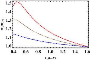
Figure 2: Variation of the non-eikonal radiation spectrum scaled by the eikonal spectrum ($\zeta$=0.0) off heavy quark ($\Delta_{M}=0.1$) with gluon transverse momentum. Red(dashed): $\zeta$=0.15; Brown(dotted): $\zeta$=0.30; Blue(dot-dashed): $\zeta$=0.45

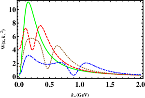
Figure 3: Variation of gluon spectrum $W(x,k_{\bot}^{2})$ off heavy quark ($\Delta_{M}=0.1,~{}x=0.1$) with gluon transverse momentum for different extents of recoil of heavy quarks. Green(solid): $\zeta$=0.0; Red(dashed): $\zeta$=0.15; Brown(dotted): $\zeta$=0.30; Blue(dot-dashed): $\zeta$=0.45

If we want to calculate the energy loss and its effect on the nuclear suppression factor we have to consider the $Qg\rightarrow Qgg$ scattering which will have more cross-section than the $Qq\rightarrow Qqg$, too. While in the eikonal case [21], the $Qg\rightarrow Qgg$ matrix element differs from that of $Qq\rightarrow Qqg$ just by a number due to color factor, the non-eikonal case is not going to be so simple and we have to calculate the Feynman amplitudes of a lot more diagrams. The present calculation may, in principle, be useful when quarks dominate in the medium. But that needs a consistent treatment of the multiple scattering process. Once that is done, we can easily find out the effect of non-eikonality in energy loss.

5 Behaviour of non-eikonal heavy quark spectrum at different kinematic regions:

Region I: Massless quark with non-eikonal trajectory

In the massless limit of Eq. LABEL:mateleQqQqg, we obtain the non-eikonal gluon radiation spectrum off light quarks. Below we jot down the forms of the functions $f_{i},\forall i=1\rightarrow 5$, $A\rightarrow D$ and $\mathcal{C}_{1},\mathcal{C}_{2},\mathcal{C}_{0}$ when we take massless limit, i.e. $m\rightarrow 0\Rightarrow\Delta_{M}\rightarrow 0$,

$$(\text{i})\mathcal{J}\rightarrow 1$$

$$(\text{ii})~{}f_{1}\rightarrow 0~{};\,f_{2}\rightarrow\frac{t}{2s}+\frac{t^{2}}{2s^{2}}+\frac{t^{3}}{4s^{3}}~{};$$

$$\,\,f_{3}\rightarrow-\frac{t}{s}-\frac{t^{2}}{2s^{2}}~{};\,\,f_{4}\rightarrow\frac{2t}{s}+\frac{3t^{2}}{2s^{2}}+\frac{t^{3}}{2s^{3}}$$

$$(\text{iii})~{}\mathcal{F}_{35}\rightarrow\mathcal{F}^{0}_{35} = 1+\left[\cot\theta\left(1-\sqrt{1-4\frac{q_{\bot}^{2}}{s}}\right)-\frac{2q_{\bot}}{\sqrt{s}}\right]\cot\frac{\theta}{2}~{};\,\,$$

$$\mathcal{F}_{45}\rightarrow\mathcal{F}^{0}_{45} = 1+\left[\cot\theta\left(1-\sqrt{1-4\frac{q_{\bot}^{2}}{s}}\right)-\frac{2q_{\bot}}{\sqrt{s}}\right]\tan\frac{\theta}{2}$$

$$(\text{iv})A\rightarrow 0~{};\,\,B\rightarrow B^{0}=-\frac{t}{2s}-\frac{t^{2}}{2s^{2}}-\frac{t^{3}}{4s^{3}}~{};$$

$$\,\,C\rightarrow C^{0}=1+\frac{t}{s}+\frac{t^{2}}{2s^{2}}~{};\,\,D\rightarrow D^{0}=1+\frac{2t}{s}+\frac{3t^{2}}{2s^{2}}+\frac{t^{3}}{2s^{3}}$$

$$(\text{v})\mathcal{C}_{1} \rightarrow \mathcal{C}_{1}^{0}=\frac{C^{0}}{4}+\frac{C^{0}}{4\mathcal{F}^{0}_{35}\mathcal{F}^{0}_{45}}+\frac{7D^{0}}{8\mathcal{F}^{0}_{35}}+\frac{7D^{0}}{8\mathcal{F}^{0}_{45}}~{};\,\,$$

$$\mathcal{C}_{2} \rightarrow \mathcal{C}_{2}^{0}=-\frac{B^{0}}{4\mathcal{F}^{0}_{35}}$$

$$\mathcal{C}_{0} \rightarrow \mathcal{C}_{0}^{0}=\frac{1}{8\mathcal{F}^{0}_{45}}\frac{t}{s}\left(1+\frac{t}{s}\left(1+\frac{t}{2s}\right)\right)$$ (18)

Hence,

$$\left|\mathcal{M}_{\mathrm{qq^{\prime}}\rightarrow\mathrm{qq^{\prime}g}}\right|^{2}=12g^{2}\frac{1}{k_{\bot}^{2}}|M_{\mathrm{qq^{\prime}}\rightarrow\mathrm{qq^{\prime}}}|^{2}\left\{\mathcal{C}_{1}^{0}+\frac{\mathcal{C}_{2}^{0}}{\tan^{2}\frac{\theta}{2}}+\mathcal{C}_{0}^{0}\tan^{2}\frac{\theta}{2}\right\}$$ (19)

If we retain the terms up to $\mathcal{O}(\frac{t}{s})$ of $B^{0},C^{0},D^{0}$ and put $\mathcal{F}_{35}=1=\mathcal{F}_{45}$, we get

$$\left|\mathcal{M}_{\mathrm{qq^{\prime}}\rightarrow\mathrm{qq^{\prime}g}}\right|^{2} = \frac{128}{27}g^{6}\frac{s^{2}}{t^{2}}\frac{1}{k_{\bot}^{2}}\left\{2\frac{1}{4}\left(1+\frac{t}{s}\right)+2\frac{7}{8}\left(1+\frac{2t}{s}\right)+\frac{t}{8s}\frac{1}{\tan^{2}\frac{\theta}{2}}+\frac{t}{8s}\tan^{2}\frac{\theta}{2}\right\}$$

$$= 12g^{2}\left\{\frac{8}{9}g^{4}\frac{s^{2}}{t^{2}}\right\}\frac{1}{k_{\bot}^{2}}\left(1+\frac{16t}{9s}+\frac{t}{9s}\cosh 2\eta\right)$$

In the limit $\eta\rightarrow 0$ Eq. LABEL:mateleqqqqgabir boils down to the light quark non-eikonal (up to $\mathcal{O}(t/s)$) matrix element obtained in Ref. [26].

Region II: Massive quark with eikonal trajectory

This region considers

$$\frac{q_{\bot}}{\sqrt{s}}\rightarrow 0\Rightarrow\frac{t}{s}\rightarrow 0$$

Hence, from Eq. 11,

$$f_{i}=0~{}\forall~{}i=1\rightarrow 5~{};\,\,\mathcal{F}_{35}=\mathcal{F}_{45}=1$$ (22)

From Eq. 13 we get, in the same limit,

$$A=B=\Delta_{M}^{2}~{};\,\,C=D=1~{};\,\,\mathcal{F}_{35}=\mathcal{F}_{45}=1$$ (23)

Hence

$$\mathcal{C}_{1}=\frac{9}{4}~{};\,\,\mathcal{C}_{2}=-\frac{9\Delta_{M}^{2}}{4}~{};\mathcal{C}_{0}=0$$ (24)

In Eq. LABEL:C_n.

With the help of Eqs. 22, 23, 24 we get,

$$\left|\mathcal{M}_{\mathrm{Qq}\rightarrow\mathrm{Qqg}}\right|^{2} = \frac{128}{27}g^{6}\frac{s^{2}}{t^{2}}\frac{1}{k_{\bot}^{2}}\frac{9}{4}\mathcal{J}^{2}$$ (25)

$$= \frac{128}{27}g^{6}\frac{s^{2}}{t^{2}}\frac{1}{k_{\bot}^{2}}(1-\Delta_{M}^{2})^{2}\frac{9}{4}\frac{1}{\left(1+\frac{\Delta_{M}^{2}}{\tan^{2}~{}\frac{\theta}{2}}\right)^{2}}$$

$$= 12g^{2}\left[\frac{8}{9}g^{4}\frac{s^{2}}{t^{2}}(1-\Delta_{M}^{2})^{2}\right]\frac{1}{k_{\bot}^{2}}\frac{1}{\left(1+\frac{\Delta_{M}^{2}}{\tan^{2}~{}\frac{\theta}{2}}\right)^{2}}$$

$$= 12g^{2}\left|\mathcal{M}_{\mathrm{Qq}\rightarrow\mathrm{Qq}}\right|^{2}\left\{\frac{1}{k_{\bot}^{2}}\left(1+\frac{m^{2}}{s}e^{2\eta}\right)^{-2}\right\}$$

with $\eta=-\ln\left(\tan~{}\frac{\theta}{2}\right)$; and the expression embraced by the curly braces is the radiated gluon spectrum ($\sim{\left|\mathcal{M}_{\mathrm{Qq}\rightarrow\mathrm{Qqg}}\right|^{2}}/{\left|\mathcal{M}_{\mathrm{Qq}\rightarrow\mathrm{Qq}}\right|^{2}}$) for this case. Evidently, the present calculation yields the calculation in Ref. [21] in the small angle scattering limit (Eq. 25).

Region III: Massless quark with eikonal trajectory

Now we explore the behaviour of the radiation spectrum in the following limits,

$$(\text{i}) \frac{q_{\bot}}{\sqrt{s}}\rightarrow 0\Rightarrow\frac{t}{s}\rightarrow 0$$

$$(\text{ii}) m=0\Rightarrow\Delta_{M}=0\Rightarrow\mathcal{J}\rightarrow 1$$

The above limits force Eq. 25 to take the form given below,

$$\left|\mathcal{M}_{\mathrm{qq^{\prime}}\rightarrow\mathrm{qq^{\prime}g}}\right|^{2} = 12g^{2}\left|\mathcal{M}_{\mathrm{Qq}\rightarrow\mathrm{Qq}}\right|^{2}\frac{1}{k_{\bot}^{2}}$$ (27)

which in the limit $q_{\bot}>>k_{\bot}$ can be written as,

$$\left|\mathcal{M}_{\mathrm{qq^{\prime}}\rightarrow\mathrm{qq^{\prime}g}}\right|^{2}\approx 12g^{2}\left|\mathcal{M}_{\mathrm{qq^{\prime}}\rightarrow\mathrm{qq^{\prime}}}\right|^{2}\left[\frac{q_{\bot}^{2}}{k_{\bot}^{2}(\vec{k}_{\bot}-\vec{q}_{\bot})^{2}}\right],$$ (28)

where $q,q^{\prime}$ are two different light quark flavors. The part within the square braces can very well be identified with the celebrated Gunion-Bertsch gluon spectrum [22] emitted from light quarks.

Region IV: Massive quark with eikonal trajectory emitting collinear gluons

This region considers the following limits

$$\text{(i)}~{}~{}m<<\sqrt{s}\Rightarrow s\approx 4E_{1}^{2}$$

$$\text{(ii)}~{}~{}\frac{q_{\bot}}{\sqrt{s}}\rightarrow 0~{}~{}\text{and}$$

$$\text{(iii)}~{}~{}\theta\rightarrow 0\Rightarrow\tan~{}\frac{\theta}{2}\approx\frac{\theta}{2}$$ (29)

In the above limit Eq. LABEL:mateleQqQqg yields the dead-cone factor of Ref. [20],

$$\left|\mathcal{M}_{\mathrm{Qq}\rightarrow\mathrm{Qqg}}\right|^{2} = 12g^{2}\left|\mathcal{M}_{\mathrm{Qq}\rightarrow\mathrm{Qq}}\right|^{2}\frac{1}{k_{\bot}^{2}}\left(1+\frac{\theta_{0}^{2}}{\theta^{2}}\right)^{-2},$$ (30)

with $\theta_{0}=\frac{m}{E_{1}}$.

6 Estimation of energy loss

In this section we calculate the eikonal and non-eikonal energy loss per unit length ($\frac{dE}{dx}$ in a medium of infinite extent) experienced by the heavy/light quarks to estimate the quantitative difference among various existing formulae in [21, 26]. Here we outline the scheme of our energy loss calculations in brief. The detailed procedures and of the energy loss calculations can be obtained in [29, 30].

We consider a thermal bath of light quarks at temperature $T=300$ MeV with which the heavy quarks interact. The interaction of the heavy quark with the light quarks is encoded in the Feynman amplitude calculated. Also, due to the presence of thermal bath, the light quarks and the radiated gluons will acquire thermal masses. We can take the quark thermal mass as $m_{f}^{2}=\pi\alpha_{s}(T)T^{2}C_{F}/2$ ; and the gluon thermal mass ($m_{g}$) is given by $m_{g}^{2}=2\pi\alpha_{s}(T)T^{2}(C_{A}+N_{f}/2)/3$ [31]. $C_{A}$($C_{F}$) is the Casimir factor in the Adjoint(Fundamental) representation and $N_{f}$ is the number of flavours.

Energy loss (per collision) due to radiated gluons can be obtained if we integrate the gluon spectrum, which is related to the ratio of the 2$\rightarrow$3 amplitude square to the 2$\rightarrow$2 amplitude square and is weighted by the gluon energy ($\omega$), over the gluon transverse momentum ($k_{\bot}$) and its rapidity ($\eta$). If we restrict ourselves within the Bethe-Heitler additive region, there will be an upper limit imposed on the $k_{\bot}$ value. The average energy loss per unit length can be obtained if we multiply the energy loss per collision with the collision rate, which we have using the techniques detailed in [32].

We observe from Fig. 4 that the inclusion of the effect of non-eikonality can result in $\sim$ 55 % ($\sim$ 39 %) change in energy loss for a 8 GeV charm quark (bottom quark) and $\sim$ 48 % ($\sim$ 43 %) change in energy loss for a 16 GeV charm quark (bottom quark).

For light quarks, the non-eikonal energy loss contains contributions from the terms of order $t^{2}/s^{2}$ and $t^{3}/s^{3}$ in the matrix element which are absent in the calculations of Ref. [26]. So, the non-eikonal energy losses of light quarks of 8 and 16 GeV differ by 24 % and 13 % respectively.

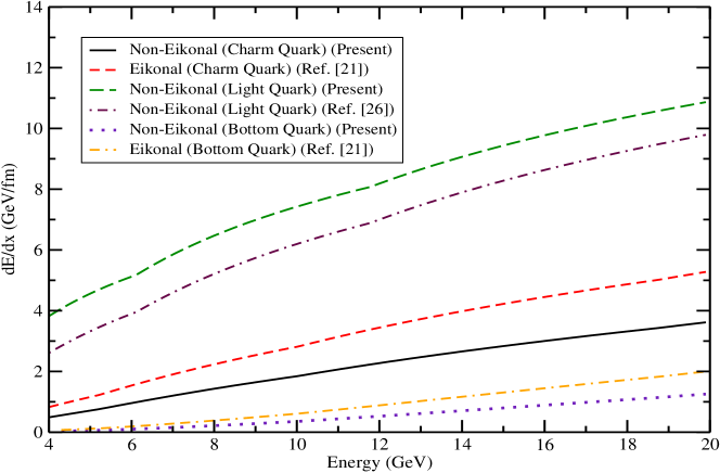
Figure 4: Energy loss of quarks in a thermal bath of 300 MeV

7 Summary and conclusion

In Summary, we have found out the non-eikonal radiation distribution off heavy quarks scattering with light quarks. Also, from Fig. 2, we realize that for soft approximations we can hardly rule out the importance of the non-eikonality. Fig. 4 shows that the effect of non-eikonality may be substantial for highly energetic heavy/light quarks. And, the consideration of the effects of non-eikonality will substantially modify the phenomenology related to the heavy-quark dynamics.

The non-eikonal distribution boils down to the all existing radiation distribution formulae provided we choose proper kinematic limits. This analysis will help towards the advancement of the continuous endeavour of relaxing the kinematic limits lingering inside the calculations of energy loss.

Unlike the eikonal case, the matrix element for the Qg$\rightarrow$Qgg process cannot be found out just by changing the color factor. The matrix element has to be evaluated for finding out non-eikonal energy loss in RHIC and LHC energy domains. The multiple scattering may be included inside the present analysis taking into account the interference effects of the scattering amplitudes due to successive collisions inside the medium. Also, recently in Ref. [33] the radiation pattern is shown to give rise to an azimuthal asymmetry which does not have any hydrodynamical origin. The present calculations may be employed to calculate the azimuthal asymmetry generated due to non-eikonality. The observed results can be compared/contrasted with the experimental findings; and that study will be the subject matter of an upcoming research paper.

References

• [1] M. Gyulassy and X. -n. Wang, Nucl. Phys. B 420, 583 (1994).
• [2] R. Baier, Y. L. Dokshitzer, A. H. Mueller, S. Peigne and D. Schiff, Nucl. Phys. B 484, 265 (1997).
• [3] B. G. Zakharov, JETP Lett.  65, 615 (1997).
• [4] M. G. Mustafa, D. Pal, D. K. Srivastava and M. Thoma, Phys. Lett. B 428, 234 (1998)
• [5] C. A. Salgado and U. A. Wiedemann, Phys. Rev. Lett.  89, 092303 (2002).
• [6] C. A. Salgado and U. A. Wiedemann, Phys. Rev. D 68, 014008 (2003).
• [7] N. Armesto, C. A. Salgado and U. A. Wiedemann, Phys. Rev. Lett.  93, 242301 (2004).
• [8] M. Gyulassy, P. Levai and I. Vitev, Nucl. Phys. B 594, 371 (2001).
• [9] M. Djordjevic and M. Gyulassy, Nucl. Phys. A 733, 265 (2004).
• [10] S. Wicks, W. Horowitz, M. Djordjevic and M. Gyulassy, Nucl. Phys. A 784, 426 (2007).
• [11] E. Wang and X. -N. Wang, Phys. Rev. Lett.  89, 162301 (2002).
• [12] X. -N. Wang and X. -f. Guo, Nucl. Phys. A 696, 788 (2001).
• [13] A. Majumder and B. Mueller, Phys. Rev. C 77, 054903 (2008).
• [14] P. B. Arnold, G. D. Moore and L. G. Yaffe, JHEP 0301, 030 (2003).
• [15] P. B. Gossiaux, R. Bierkandt and J. Aichelin, Phys. Rev. C 79, 044906 (2009).
• [16] M. Younus and D. K. Srivastava, J. Phys. G 39, 095003 (2012).
• [17] R. Abir, U. Jamil, M. G. Mustafa and D. K. Srivastava, Phys. Lett. B 715, 183 (2012).
• [18] S. Cao, G. Y. Qin and S. A. Bass, Phys. Rev. C 88, 044907 (2013)
• [19] Y. L. Dokshitzer, V. A. Khoze and S. I. Troyan, J. Phys. G: Nucl. Part. Phys. 17, 1602(1991)
• [20] Y. L. Dokshitzer and D. E. Kharzeev, Phys. Lett. B 519, 199 (2001)
• [21] R. Abir, C. Greiner, M. Martinez, M. G. Mustafa and J. Uphoff, Phys.Rev. D 85, 054012(2012)
• [22] J. F. Gunion and G. Bertsch, Phys. Rev. D 25, 746 (1982).
• [23] S. K. Das, J. e. Alam and P. Mohanty, Phys. Rev. C 82, 014908 (2010)
• [24] S. Mazumder, T. Bhattacharyya, J. e. Alam and S. K. Das, Phys. Rev. C 84, 044901 (2011)
• [25] K. Saraswat, P. Shukla and V. Singh, Nucl. Phys. A 943, 83 (2015)
• [26] R. Abir, Phys. Rev. D 87, 034036(2013).
• [27] S. K. Das and J. Alam, Phys. Rev. D 82, 051502(R), (2010).
• [28] R. Abir, C. Greiner, M. Martinez, and M. G. Mustafa, Phys. Rev. D 83, 011501 (R) (2011)
• [29] T. Bhattacharyya, S. Mazumder J. Alam and S. K. Das, Phys. Rev. D 85, 034033 (2012)
• [30] X. N. Wang, M. Gyulassy and M. Plumer, Phys. Rev. D 51, 3436 (1995)
• [31] M. Le Bellac, Thermal Field Theory, Cambridge University Press, Cambridge 1996.
• [32] M. H. Thoma, Phys. Rev. D 49, 451(1994)
• [33] T. S. Birò, M. Horvàth, Zs. Schram, Eur. Phys. J. A 51 (2015) 75