Casimir interaction at liquid nitrogen temperature: Comparison between experiment and theory

Abstract

We have measured the normalized gradient of the Casimir force between Au-coated surfaces of the sphere and the plate and equivalent Casimir pressure between two parallel Au plates at $T=77\,$K. These measurements have been performed by means of dynamic force microscope adapted for operating at low temperatures in the frequency shift technique. It was shown that the measurement results at $T=77\,$K are in a very good agreement with those at $T=300\,$K and with computations at $T=77\,$K using both theoretical approaches to the thermal Casimir force proposed in the literature. No thermal effect in the Casimir pressure was observed in the limit of experimental errors with the increase of temperature from $T=77\,$K to $T=300\,$K. Taking this into account, we have discussed the possible role of patch potentials in the comparison between measured and calculated Casimir pressures.

I Introduction

Rapid progress in nanotechnology has resulted in the growth of interest in fluctuation-induced phenomena which can play a dominant role at short separation distances below a micrometer.1 ; 2 Among these phenomena a particular attention is focussed on the Casimir effect3 which manifests itself as a force acting between two uncharged closely spaced material boundaries. The Casimir force is caused by zero-point and thermal fluctuations of the electromagnetic field. In the first approximation it depends only on the velocity of light $c$, Planck constant $\hbar$, temperature $T$ and separation distance $a$ between the test bodies. A more exact theory demonstrates dependence of the Casimir force on the material properties of the bodies 4 and geometry of their boundary surfaces.5 ; 6

Taking into account both fundamental interest and potential applications in nanotechnology, many experiments have been performed on measuring the Casimir force (see the monograph7 and reviews8 ; 9 ; 10 ). Specifically, measurements with different levels of precision were done between two metallic surfaces (see, e.g., Refs. 11 ; 12 ; 13 ; 14 ; 15 ; 16 ) and between a metallic and a semiconductor surfaces (see, e.g., Refs. 17 ; 18 ; 19 ; 20 ; 21 ; 22 ; 23 ; 24 ). Quite unexpectedly, the experimental data of many experiments performed at room temperature13 ; 15 ; 16 ; 18 ; 23 ; 24 ; 25 ; 26 were found to exclude the theoretical predictions taking into account the relaxation properties of conduction electrons for metals and the contribution of free charge carriers for semiconductors of the dielectric type. The same data were found to be consistent with theory neglecting the relaxation properties of conduction electrons for metals and the free charge carriers for dielectric-type semiconductors (the two experiments which claim confirmation of the role of relaxation properties of free electrons for metallic test bodies27 ; 28 are critically discussed in the literature29 ; 30 ; 31 ; 32 ). Coincident with the experimental work, it was shown33 ; 34 that the account of relaxation properties for metals and free charge carriers for dielectrics leads to violation of the Nernst heat theorem (the third law of thermodynamics) in the Lifshitz theory. These results have led to a critical discussion (see, e.g., Refs. 35 ; 36 ; 37 ; 38 ) which continues to the present day. Specifically, it was hypothesized39 that the effect of large surface patches might bring the measurement data25 in agreement with theory taking the relaxation properties of electrons into account. However, measurements of the Casimir force between magnetic surfaces16 ; 40 demonstrated that this suggestion does not lead to the desired result.

Keeping in mind that the problems discussed above are connected with thermal dependence of the Casimir force, it would be elucidating to perform experiments at different temperatures $T$. Measurements at varying $T$ cannot entirely resolve the theoretical problem of the Nernst theorem because experimentally it is not possible to achieve arbitrarily low temperatures. Such measurements, however, can be helpful in many aspects, specifically, for understanding the Casimir effect between superconducting test bodies. A suggestion to measure the Casimir force at different $T$ was proposed a decade ago41 but remained unrealized due to experimental difficulties. Recently, however, some progress in measuring the Casimir force at low temperatures has been achieved. Thus, the effective Casimir pressure between two parallel plates was determined42 at $T=2.1\,$K, 4.2 K and 77 K by means of a micromachined oscillator. This was done dynamically by measuring the change in resonant frequency of an Au sphere oscillating near an Au plate with the help of the proximity force approximation (PFA)7 ; 8 (note that recently the applicability of PFA for the configuration of a sphere and a plate made of real materials was confirmed to a high precision43 ; 44 ; 45 ; 46 ). It was shown42 that although the low temperature data are noisier than at room temperature, the mean measured Casimir pressures coincide at all temperatures. Thus, it was experimentally demonstrated that within a wide temperature region there is no thermal effect in the Casimir pressure exceeding the measurement errors (no comparison with theory has been made).

In fact at short separation distances the predicted thermal effect depends on the theoretical approach, but in all cases it is rather small. Thus, for Au plates with neglected relaxation properties of free electrons (the so-called plasma model approach, see Sec. III) spaced at separation $a\lesssim 500\,$nm the relative thermal correction to the Casimir pressure at $T=77\,$K is less than 0.006%. At $T=300\,$K the thermal correction varies from 0.02 mPa (0.0026%) at $a=180\,$nm to 0.005 mPa (0.03%) at $a=500\,$nm. Such thermal corrections cannot be measured by the presently existing experimental means. For Au plates with included relaxation properties of free electrons (the so-called Drude model approach, see Sec. III) at $T=77\,$K the thermal correction varies from –5.8 mPa (–0.77%) at $a=180\,$nm to –0.35 mPa (–2%) at $a=500\,$nm. At room temperature $T=300\,$K the thermal correction calculated using the Drude model approach achieves –17 mPa (–2.3%) at $a=180\,$nm and –1.3 mPa (–7.7%) at $a=500\,$nm. If such corrections were really exist, they could be observed experimentally using available setups.

Furthermore, measurements of the gradient of the Casimir force between an Au sphere and either an Au or a doped Si plate was performed47 at $T=4.2\,$K by means of dynamic atomic force microscope (AFM). The experimental data were compared with theory taking the relaxation properties of charge carriers into account, but were found above the theoretical curve by 50%, i.e., much more than the experimental error. It was suggested that a possible source of disagreement with theory is the unaccounted error in calibration of the piezoelectric scanner extension.

Next, the dynamic AFM was adopted48 for precise measurements of the gradient of the Casimir force between Au surfaces of the sphere and the plate in a wide temperature region from 5 K to 300 K. Unlike the previous work,47 the developed instrument measured the extension of the piezoelectric scanner in real time during measurements of the Casimir interaction. This has helped to avoid any unaccounted systematic errors in the measurement. Some preliminary measurements were performed48 at $T=6.7\,$K and demonstrated an agreement with the measurement results at $T=300\,$K within the limits of experimental errors.

In this paper we use the instrument designed in Ref. 48 , which can operate between 5 K and 300 K, for systematic measurements of the normalized gradient of the Casimir force between sphere and plate at a liquid nitrogen temperature $T=77\,$K. This is done by means of dynamic AFM operated in the frequency shift mode. In contrast to all previous measurements of the Casimir interaction at low temperature, here we present the detailed analysis of both random and systematic errors and the comparison between the experimental data and predictions of different theoretical approaches to the thermal Casimir force. We demonstrate that the mean values of our data are in an excellent agreement with the respective means at room temperature and with predictions of both theoretical approaches at $T=77\,$K (note that the difference between the latter at a liquid nitrogen temperature is well below the experimental error). The importance of these results for the problem of thermal Casimir force is discussed.

The paper is organized as follows. In Sec. II we briefly consider the low-temperature setup for measurements of the Casimir interaction and present the measurement scheme. Section III contains the measurement data at $T=77\,$K, the error analysis and the comparison between experiment and theory. In Sec. IV the reader will find our conclusions and discussion.

II Measurement setup at low temperature and measurement scheme

We have used dynamic AFM operated in the frequency shift technique to measure the gradient of the Casimir force normalized to the sphere radius between an Au-coated hollow microsphere and an Au-coated sapphire plate at $T=77\,$K. The experimental setup has been described in detail elsewhere.48 In brief, however, the device we use to measure the Casimir force gradient is a variable-temperature force sensor (VTFS). The apparatus is based on the AFM technique but particularly designed to precisely measure the Casimir force gradient at temperatures in the 5 K to 300 K range. Here measurements are done at 77 K. These measurements were performed at a vacuum pressure of $\lesssim 10^{-6}\,$Torr using an oil-free vacuum chamber. The measurement system was vibrationally isolated using a double-stage spring system. Low temperatures were achieved by immersing the VTFS vacuum chamber in a liquid nitrogen Dewar. The sensor consists of a modified conductive Si rectangular microcantilever.48

The Casimir force gradient was measured between a sphere and a plate both coated with Au. A hollow glass sphere of $R\approx 50\,\mu$m radius made from liquid phase was attached to the end of a rectangular Si cantilever. The sphere-cantilever system was coated uniformly with greater than 100 nm of Au. The low inertia of the hollow sphere leads to higher cantilever resonant frequencies and mechanical $Q$ factors, both of which result in improved sensitivities. Care should be taken to restrict the Au coating to only the cantilever tip. The cantilever with the attached sphere had a quality factor $Q=871$ and a resonant frequency of $\omega_{0}=2\pi\times 2.766\,\mbox{kHz}=17.379\,$krad/s.

An Au-coated sapphire plate was used as the second surface. The thickness of the Au coating on the plate was $260\pm 1\,$nm. The Au plate was mounted at a top of a piezoelectric ceramic tube. The fabrication and characterization methods for both surfaces have been reported in the literature.15 ; 48 ; 49 The Casimir interaction was obtained through the direct measurement of the shift of the microcantilever’s resonant frequency while the cantilever was being lightly driven with an amplitude of 10 nm at its resonance frequency.50 The microcantilever oscillation was detected with an all-fiber interferometer.48 The resulting signal was analyzed and controlled through a closed-loop feedback system provided by a phase-lock loop (PLL). The PLL detection bandwidth was kept at 50 Hz. The output of the feedback loop was the resonant-frequency shift, $\omega_{r}(a)-\omega_{\rm PLL}$ where $\omega_{r}(a)$ is the resonance frequency in the presence of an external force and $\omega_{\rm PLL}$ is some frequency fixed during the measurements. It is convenient to keep it close but not equal to $\omega_{0}$.

Different voltages were applied to the plate, while the sphere remained grounded. The resonant-frequency shifts were measured for different separations and DC voltages between the interacting surfaces. The separation distance between the sphere and plate was changed continuously by applying a 10 mHz triangular voltage signal to the piezoelectric tube holding the Au-coated sapphire plate. The movement of the plate was monitored in real time and calibrated with a second all-fiber interferometer48 using $636.8\pm 0.4\,$nm wavelength light.

The relative distance moved by the piezo was calibrated with an end cleaved fiber interferometer. We fitted the interference voltage to third order with a cosine function using the $\chi^{2}$-fitting procedure. The obtained fitting parameters were used for calibration of piezo. First, 11 voltages from 0.56 to 0.68 V were applied to the plate while the sphere remained grounded. In addition, 9 repititions of 0.62 V were also applied to the plate, maintaining the sphere grounded. The frequency shift was measured as a function of the distance moved by the piezo at every 2.45 nm for each applied voltage. The set of measurements with 20 applications of the voltage to the plate was repeated 3 times and one time more with 19 applied voltages. A total of 79 runs for the frequency shift as a function of separation were taken. We confirmed that at large separations between $2.2\,\mu$m and $2.6\,\mu$m the frequency shift $\omega_{r}(a)-\omega_{\rm PLL}$ remains constant within the resolution limit. This means that at separations above $2.2\,\mu$m $\omega_{r}(a)=\omega_{0}$.

In the linear regime which occurs for small amplitudes of the cantilever the frequency shift is given by

$$\Delta\omega(a)=-\frac{\omega_{0}}{2k}\,\frac{\partial F_{\rm tot}(a)}{\partial a}\equiv-\frac{\omega_{0}}{2k}F_{\rm tot}^{\prime}(a).$$ (1)

Here, $k$ is the spring constant of the cantilever, $a$ is the absolute sphere-plate separation distance (including the relative distance moved by the plate piezo, $z_{\rm piezo}$, and the closest distance $z_{0}$), and the frequency shift between $\omega_{r}(a)$ and $\omega_{0}$ is determined according to the following equation:

$$\Delta\omega(a)\equiv\omega_{r}(a)-\omega_{0}=[\omega_{r}(a)-\omega_{\rm PLL}]-(\omega_{0}-\omega_{\rm PLL}).$$ (2)

The total force between the sphere and the plate is the sum of the electrostatic force $F_{\rm el}(a)$ and the Casimir force $F_{C}(a)$

$$F_{\rm tot}(a)=F_{\rm el}(a)+F_{C}(a).$$ (3)

The electric force between the sphere and the plate is expressed as

$$F_{\rm el}(a)=X(a,R)(V_{i}-V_{0})^{2},$$ (4)

where $V_{0}$ is the residual potential difference between the bodies, which can be caused by the various connections and by different work functions of a sphere and a plate materials, and $X(a,R)$ is an explicitly known function.7 ; 8 Using the expansion of this function in powers of a small parameter $a/R$ obtained in the literature,7 ; 8 ; 17 we can rewrite Eq. (1) in the form

$$\Delta\omega(a)=-\frac{\omega_{0}}{2k}F_{C}^{\prime}(a)-\frac{\omega_{0}}{2k}\,\frac{\partial X(a,R)}{\partial a}(V_{i}-V_{0})^{2}$$ (5)

$$~{}~{}=-\frac{\tilde{C}}{2\pi R}F_{C}^{\prime}(a)-\frac{\tilde{C}\epsilon_{0}}{2a^{2}}\left[1-\sum_{i=1}^{6}ic_{i}\left(\frac{a}{R}\right)^{i+1}\right](V_{i}-V_{0})^{2}.$$

Here, $\tilde{C}\equiv\pi\omega_{0}R/k$ is the calibration constant [we label $C$ with a tilde to indicate the difference with $C=\omega_{0}/(2k)$ used in the literature15 ; 16 ; 40 ], $\epsilon_{0}$ is the permittivity of free space and the numerical coefficients $c_{i}$ can be found in Refs. 7 ; 8 ; 17 .

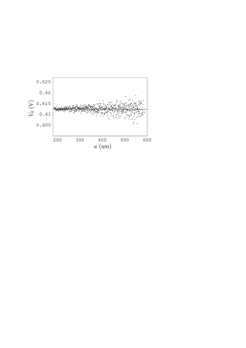
Figure 1: The residual potential difference $V_{0}$ between an Au-coated sphere and an Au-coated plate at $T=77\,$K as a function of separation. The best fit of $V_{0}$ to the straight line is shown by the solid line.

Any mechanical or thermal drift of the piezo leading to a change in the sphere-plate separation distance was found to be $1.11226\pm 0.00455\,$nm/hour. The corresponding corrections to this small drift were done as reported previously.15 After applying the drift correction, the residual potential $V_{0}$ was found at each separation from the parabolic dependence of the measured frequency shift on $V_{i}$. The value of $V_{0}$ at a fixed separation can be identified as the position of the parabola maximum. The obtained $V_{0}$ as a function of separation is shown by dots in Fig. 1. As is seen in the figure, the mean $V_{0}=0.6125\pm 0.0015\,$V is independent of separation over the entire measurement range. To quantify this observation, we have performed the best fit of $V_{0}$ to the straight line leaving its slope as a free parameter (solid line in Fig. 1). It was found that the slope is equal to $-5.7\times 10^{-7}\,$V/nm, i.e., the independence of $V_{0}$ on separation was confirmed to a high precision.

The curvature of the parabolas of the measured frequency shift as a function of $V_{i}$ corresponds to the spatial dependence of the electrostatic force and the force calibration constant $\tilde{C}$. In accordance with Eq. (5), this parabola curvature was fitted to the quantity

$$\beta\equiv\frac{\tilde{C}\epsilon_{0}}{2a^{2}}\left[1-\sum_{i=1}^{6}ic_{i}\left(\frac{a}{R}\right)^{i+1}\right]$$ (6)

in order to determine the calibration constant $\tilde{C}$ and the closest mean sphere-plate separation $z_{0}$ taking into account that $a=z_{0}+z_{\rm piezo}$. The fitting procedure was repeated by keeping the start point fixed at the closest separation, while the end point $z_{\rm end}$ measured from the closest separation was varied over a wide range. Similar to Ref. 15 , $z_{0}$ and $\tilde{C}$ so determined were shown to be independent on $z_{\rm end}$. The obtained values of the calibration parameters are $z_{0}=184.4\pm 1.5\,$nm and $\tilde{C}=78.2\pm 1.0\,\mbox{rad\,m}^{2}/$N s). The errors are determined by the systematic errors in the fit.

The Casimir force and electrostatic force between sphere and plate are both attractive and cause the cantilever to bend towards the plate by around 1 nm at the maximum applied voltage at the closest separation. Here, there was no real time correction of the cantilever bending using a proportional integral derivative loop, as reported in Ref. 15 . Thus, for a precise measurement, all the values of absolute separations $a$ have to be corrected for this bending. The correction was done in the following manner. By integrating Eq. (1) from $a$ to $\infty$ we can get

$$F_{\rm tot}(a)=\frac{2k}{\omega_{0}}\int_{a}^{\infty}\!\!\Delta\omega(z)\,dz,$$ (7)

where $a<L=2.2\,\mu$m and $L$ is the largest distance at which the frequency shift was measured. Keeping in mind that at $a\geq L$ the Casimir force is nearly equal to zero, from Eq. (3) we obtain $F_{\rm tot}(a)\approx F_{\rm el}(a)$ and then

$$\frac{2k}{\omega_{0}}\int_{L}^{\infty}\!\!\Delta\omega(z)\,dz\approx F_{\rm el}(L).$$ (8)

Subdividing the integration region in Eq. (7) in two subregions $[a,L]$ and $[L,\infty)$ and using Eq. (8), we rewrite Eq. (7) in the form

$$F_{\rm tot}(a)\approx\frac{2k}{\omega_{0}}\int_{a}^{L}\!\!\Delta\omega(z)\,dz+F_{\rm el}(L).$$ (9)

Finally, with the help of Eq. (4), Hooke’s law and the expansion of the function $X(a,R)$ in powers of a small parameter,7 ; 8 ; 17 one arrives to the following bending distance of the cantilever:

$$b(a)=\frac{F_{\rm tot}(a)}{k}=\frac{2}{\omega_{0}}\int_{a}^{L}\!\!\Delta\omega(z)\,dz+\frac{F_{\rm el}(L)}{k}$$ (10)

$$~{}~{}~{}=\frac{2}{\omega_{0}}\int_{a}^{L}\!\!\Delta\omega(z)\,dz-\frac{\tilde{C}\epsilon_{0}}{\omega_{0}L}\left[1+\sum_{i=0}^{6}c_{i}\left(\frac{L}{R}\right)^{i+1}\right](V_{i}-V_{0})^{2}.$$

Now we can use Eq. (10) to correct all the values of absolute separation $a=a_{0}=z_{0}+z_{\rm piezo}$ at any applied voltage for a bending of the cantilever by means of an iteration procedure. First we substitute $a_{0}$ (zero iteration) in Eq. (10) and calculate $b(a_{0})$ at any $z_{\rm piezo}$. The first iteration of absolute separations is defined as $a_{1}=a_{0}-b(a_{0})$. Substituting this in Eq. (10), we find $b(a_{1})$ etc. In the iteration number $i$ we have $a_{i}=a_{i-1}-b(a_{i-1})$. This is iterated until the obtained value converge at any $z_{\rm piezo}$ and any applied voltage. Note that for all separations and applied voltages the correction due to the bending of the cantilever is smaller than 1 nm and decreases with increasing separation. Thus, it is below the error in the determination of absolute separations. The obtained values of all calibration parameters $V_{0}$, $\tilde{C}$, $z_{0}$ and absolute separations $a$ can now be used to perform an independent measurement of the Casimir interaction at the liquid nitrogen temperature.

III Measurement data, error analysis and comparison with theory

As discussed in Sec. II, the frequency shift $\Delta\omega$ caused by the combined action of the electric and Casimir forces was measured as a function of separation 79 times with different applied voltages over the separation region from 187 nm to $2.2\,\mu$m. Then the normalized gradients of the Casimir force, $F_{C}^{\prime}(a)/(2\pi R)$, at different separations were found from Eq. (5). For comparison purposes, it is convenient to recalculate the normalized gradients of the Casimir force in sphere-plate geometry into the Casimir pressure $P_{C}(a)$ between two Au-coated plane parallel plates. This can be done by means of the PFA7 ; 8

$$F_{C}(a)=2\pi RE_{C}(a),$$ (11)

where $E_{C}(a)$ is the Casimir energy per unit area of two parallel plates. The negative differentiation of both sides of Eq. (11) leads to the desired result

$$P_{C}(a)=-\frac{1}{2\pi R}F_{C}^{\prime}(a),$$ (12)

i.e., the Casimir pressure coincides with the negative normalized gradient. At separations of several hundred nanometers, important for this experiment, the error introduced by the use of PFA does not exceed a fraction of a percent43 ; 44 ; 45 ; 46 , i.e., much less than the experimental error (see below).

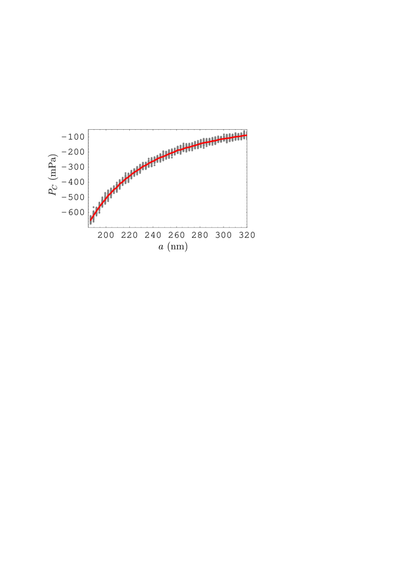
Figure 2: (Color online) All 79 individual values of the Casimir pressure at $T=77\,$K measured at each point are shown as gray dots with a step of 2.45 nm. The mean measured Casimir pressure as a function of separation is indicated by the solid line.

In Fig. 2 all 79 individual values of the Casimir pressure measured at each point are shown at short separation distances as gray dots with a step of 2.45 nm. In the same figure the mean values of the measured Casimir pressure at each separation are interpolated and presented as the solid line.

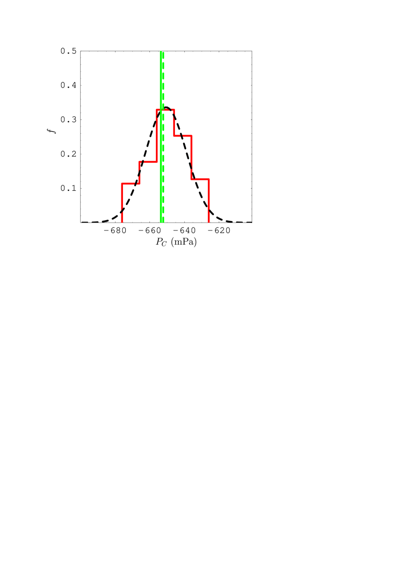
Figure 3: (Color online) The histogram for the measured Casimir pressure at $T=77\,$K at the separation $a=187\,$nm. The corresponding Gaussian distribution is shown by the dashed curve. The solid and dashed vertical lines indicate the theoretical predictions from the plasma and Drude model approaches, respectively (see text for further discussion).

The statistical properties of the measurement data for the Casimir pressure are characterized by the histogram in Fig. 3 plotted at $a=187\,$nm. Here, $f$ is the fraction of 79 data points having the force values in the bin indicated by the respective vertical lines. The histogram is described by the Gaussian distribution with the standard deviation equal to $\sigma_{P_{C}}=11.5\,$mPa and the mean Casimir pressure $\bar{P}_{C}=-650.65\,$mPa (see also below for the comparison with predictions of different theoretical approaches indicated in Fig. 3 by the solid and dashed vertical lines).

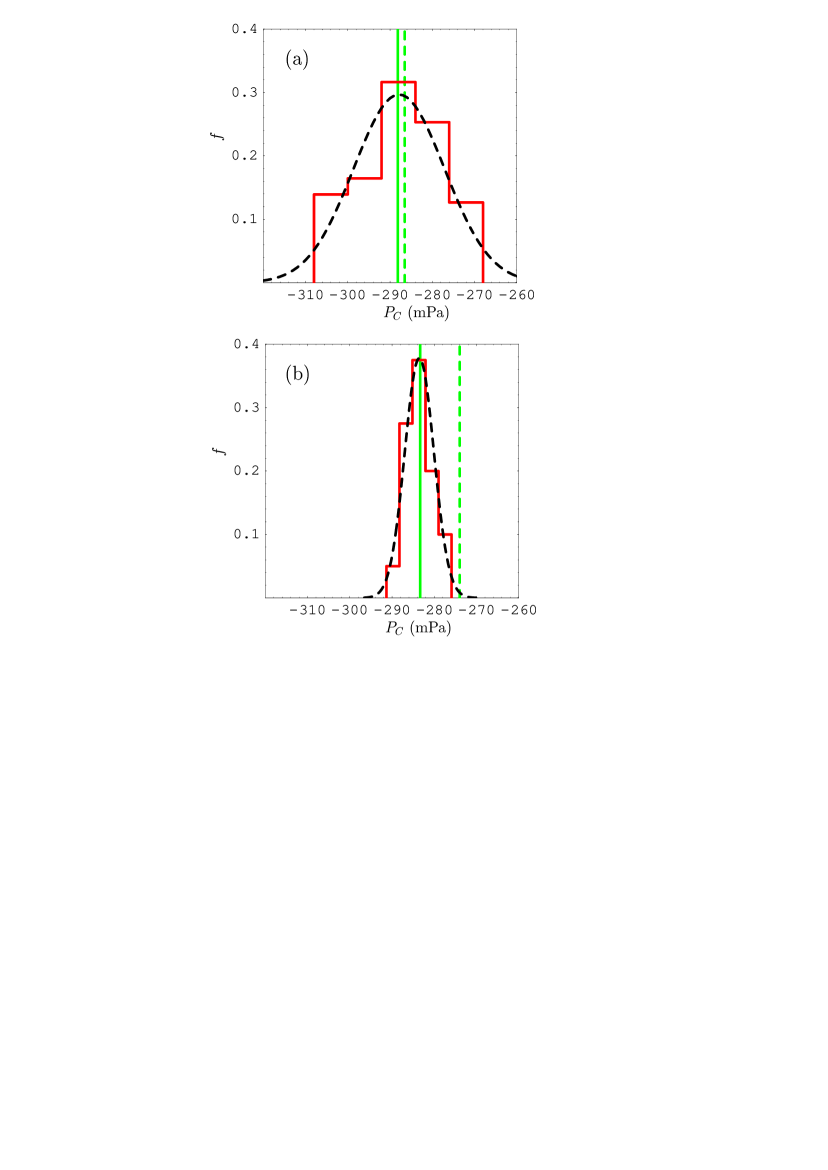
Figure 4: (Color online) The histogram for the measured Casimir pressure (a) at $a=234\,$nm, $T=77\,$K and (b) $a=235\,$nm, $T=300\,$K measured in this work and in Ref. 15 , respectively. The corresponding Gaussian distributions are shown by the dashed curves. The solid and dashed vertical lines indicate the theoretical predictions from the plasma and Drude model approaches, respectively (see text for further discussion).

It is instructive to compare the measurement data at $T=77\,$K and $T=300\,$K. This is done in Fig. 4(a,b) where the two histograms are presented at $a=234\,$nm, $T=77\,$K (this work) and at $a=235\,$nm, $T=300\,$K (by the results of Ref. 15 ), respectively. The respective standard deviations and mean Casimir pressures are $\sigma_{P_{C}}=10.5\,$mPa, $\bar{P}_{C}^{\rm expt}=-287.87\,$mPa [$T=77\,$K, Fig. 4(a)] and $\sigma_{P_{C}}=2.75\,$mPa, $\bar{P}_{C}^{\rm expt}=-284.17\,$mPa [$T=300\,$K, Fig. 4(b)]. As can be seen from the comparison of Fig. 4(a) and Fig. 4(b), at $a\approx 235\,$nm the mean Casimir pressures measured at the liquid nitrogen and room temperatures are in very good agreement although the data at $T=77\,$K are less precise.

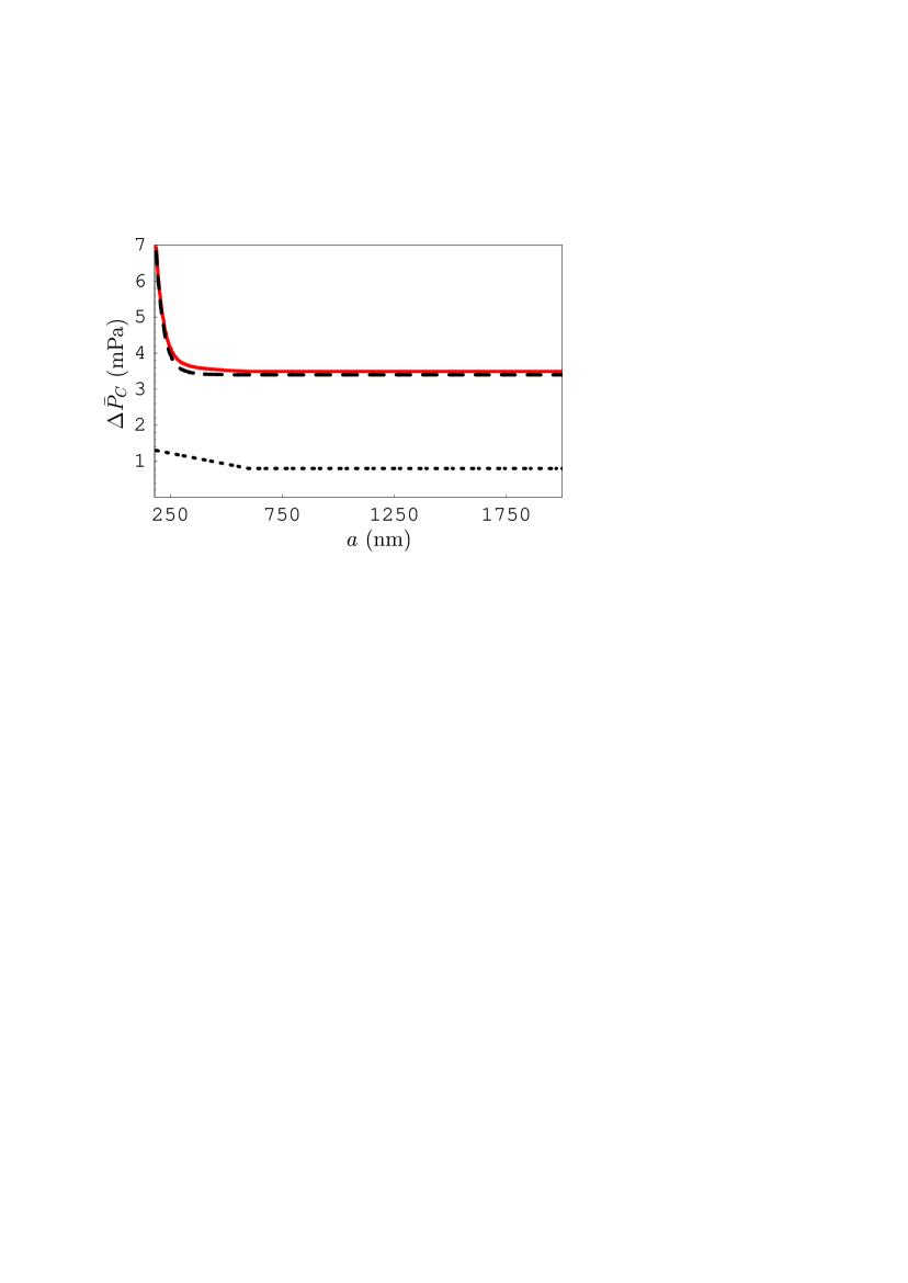
Figure 5: (Color online) The random, systematic and total experimental errors in the measured mean Casimir pressure at 77 K determined at a 67% confidence level are shown by the dotted, dashed, and solid lines, respectively.

To compare our experimental data with the data of other experiments and with theory over wide separation regions, we first analyze the experimental errors. The random error in the measured Casimir pressure is calculated by using Student’s distribution. As a function of separation, the random error determined at a 67% confidence level is shown by the dotted line in Fig. 5. The largest value of the random error equal to 1.3 mPa is achieved at the shortest separation $a=187\,$nm. Then it decreases down to 0.8 mPa when separation increases up to 600 nm and preserves this value at larger separations. The systematic error in this experiment is determined by the instrumental noise including the background noise level and by the errors in calibration. In Fig. 5 the systematic error is shown by the long-dashed line. As can be seen in this figure, the systematic error achieves the largest value of 6.8 mPa at $a=187\,$nm, decreases to 4.0 mPa at $a=250\,$nm and is equal to 3.4 mPa at all separation distances larger than 340 nm. We emphasize that the systematic error in this experiment is larger than in previously performed experiment15 by means of AFM at $T=300\,$K (where it was approximately equal to 1.8–1.9 mPa). The significant increase of the systematic error in the low-temperature setup, as compared to the room temperature, is due to internal vibrations when the cryogenic liquid is present.42 By adding the random and systematic errors in quadrature, we obtain the total experimental error in the measured Casimir pressure determined at a 67% confidence level. It is shown by the solid line in Fig. 5. The total error is mostly determined by the systematic error. It is equal to 6.9 mPa at $a=187\,$nm, decreases to 4.1 mPa at $a=250\,$nm, and preserves the value of 3.5 mPa at all separations exceeding 450 nm.

Now we plot our mean experimental data as crosses in Fig. 6(a,b), where the vertical arms are equal to the total experimental error in the measured Casimir pressure and the horizontal arms are equal to the error in the measurement of separations $\Delta a=\Delta z_{0}=1.5\,$nm (the error in $z_{\rm piezo}$ is negligibly small). The separation regions are chosen for the comparison with the mean measured Casimir pressures of Ref. 15 and Refs. 25 ; 26 shown by the solid lines in Figs. 6(a) and 6(b), respectively. As can be seen in Fig. 6(a,b), our measurement data at $T=77K$ are in a very good agreement in the limits of experimental errors with the measurement data of Ref. 15 obtained by means of AFM and Refs. 25 ; 26 obtained by means of micromachined oscillator at $T=300\,$K. This demonstrates that there is a mutual agreement between all these experiments and that there is no thermal effect exceeding the measurement errors when the temperature increases from 77 K to 300 K.

Next we compare the measurement data for the mean Casimir pressure with theory. The thickness of Au coatings is large enough to consider our effective parallel plates as semispaces made of gold.7 The Lifshitz formula for the Casimir pressure between two semispaces at temperature $T$ is given by4 ; 7 ; 8 ; 9

$$P_{C}(a)=-\frac{k_{B}T}{\pi}\sum_{l=0}^{\infty}{\vphantom{\sum}}^{\prime}\int_{0}^{\infty}\!q_{l}k_{\bot}dk_{\bot}\sum_{\alpha}\frac{r_{\alpha}^{2}}{e^{2aq_{l}}-r_{\alpha}^{2}},$$ (13)

where $k_{B}$ is the Boltzmann constant and the laboratory temperature is $T=77\,$K. The quantity $q_{l}^{2}=k_{\bot}^{2}+\xi_{l}^{2}/c^{2}$ where $k_{\bot}$ is the projection of the wave vector on the plane of plates, and $\xi_{l}=2\pi k_{B}Tl/\hbar$ with $l=0,\,1,\,2,\,\ldots$ are the Matsubara frequencies. The prime near the first summation sign multiplies the term with $l=0$ by 1/2, and the second summation sign summarizes over the transverse magnetic ($\alpha={\rm TM}$) and transverse electric ($\alpha={\rm TE}$) polarizations of the electromagnetic field. The reflection coefficients $r_{\alpha}$ are calculated along the imaginary frequency azis. They are given by

$$r_{\rm TM}\equiv r_{\rm TM}(i\xi_{l},k_{\bot})=\frac{\varepsilon(i\xi_{l})q_{l}-k_{l}}{\varepsilon(i\xi_{l})q_{l}+k_{l}},$$

$$r_{\rm TE}\equiv r_{\rm TE}(i\xi_{l},k_{\bot})=\frac{q_{l}-k_{l}}{q_{l}+k_{l}},$$ (14)

where the dielectric permittivity of Au calculated at the imaginary Matsubara frequencies is $\varepsilon(i\xi_{l})$ and

$$k_{l}=\left[k_{\bot}^{2}+\varepsilon(i\xi_{l})\frac{\xi_{l}^{2}}{c^{2}}\right]^{1/2}.$$ (15)

As discussed in Sec. I, there are two approaches on how to apply the Lifshitz theory to metallic bodies. The Drude model approach7 ; 8 ; 35 ; 36 takes into account the relaxation properties of conduction electrons. In the framework of this approach, the optical data of boundary metal are extrapolated down to zero frequency by means of the Drude model and are used to calculate $\varepsilon(i\xi_{l})$ with the help of the dispersion relation. The tabulated optical data51 of Au are well extrapolated52 by the Drude model with the plasma frequency $\omega_{p}=9.0\,$eV and relaxation parameter $\gamma=0.035\,$eV determined at $T=300\,$K. [Note that although $\omega_{p}$ is temperature-independent, the relaxation parameter decreases with decreasing temperature, so that $\gamma(77\,\mbox{K})\approx 0.9\,$meV.] The consistency of this extrapolation was recently confirmed by using the weighted Kramers-Kronig relations.53 The immediately measured optical data for Au films, similar to those used in experiments of Refs. 15 ; 25 ; 26 , by means of ellipsometry lead to the same Casimir pressures as the tabulated optical data.42 In the framework of the plasma model approach, the same optical data with the contribution of free charge carriers subtracted are extrapolated down to zero frequency by means of the plasma model with the same $\omega_{p}$.

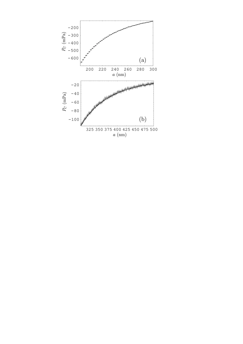
Figure 7: Comparison between the mean experimental data for the Casimir pressure at $T=77\,$K (crosses plotted at a 67% confidence level) and the common theoretical prediction of the Drude and plasma model approaches at $T=77\,$K (solid lines) within the separation region (a) from 187 to 300 nm and (b) from 300 to 500 nm.

We have calculated the Casimir pressure at $T=77\,$K using Eqs. (13)–(15) over the entire measurement region from 187 nm to $2\,\mu$m in the framework of both approaches (note that the surface roughness in this experiment contributes a small fraction of a percent and can be neglected in comparison to the error bars15 ). The computational results are presented by the solid lines in Fig. 7(a) within the separation region from 187 to 300 nm and in Fig. 7(b) within the region from 300 to 500 nm. We emphasize that with the scale used the differences between predictions of the Drude and plasma model approaches are below resolution. In the same figures, the experimental data are shown as crosses, as discussed above. From Fig. 7(a,b) it can be seen that the measured mean Casimir pressures are in good agreement with theory. In order to trace the differences between the predictions of the Drude and plasma model approaches, we return to Figs. 3 and 4 where both predictions are shown by the dashed and solid vertical lines, respectively. In Fig. 3 ($a=187\,$nm), $P_{D}^{\rm th}=-652.25\,$mPa and $P_{p}^{\rm th}=-653.61\,$mPa leading to only a 1.36 mPa difference. This is much smaller than the total experimental error at this separation (6.9 mPa) and also smaller than the theoretical error equal to 3.3 mPa.

To compare the predictions of both computational approaches at $T=77\,$K and $T=300\,$K one should look to Figs. 4(a) and 4(b), respectively. In Fig. 4(a), one has $P_{D}^{\rm th}(T=77\,\mbox{K})=-286.53\,$mPa and $P_{p}^{\rm th}(T=77\,\mbox{K})=-288.16\,$mPa. This leads to a 1.63 mPa difference still smaller than the total experimental error $\Delta^{\!\rm tot}\bar{P}_{C}^{\rm expt}(T=77\,\mbox{K})=4.4\,$mPa. In contrast in Fig. 4(b) plotted at $T=300\,$K, $P_{D}^{\rm th}(T=300\,\mbox{K})=-273.99\,$mPa and $P_{p}^{\rm th}(T=300\,\mbox{K})=-283.35\,$mPa leading to the difference of 9.36 mPa much larger than the total experimental error in this experiment equal to $\Delta^{\!\rm tot}\bar{P}_{C}^{\rm expt}(T=300\,\mbox{K})=1.9\,$mPa. [Note that the difference between the plasma model predictions in Figs. 4(a) and 4(b) is equal to –4.81 mPa; the major part of this –4.82 mPa, is due to the change of separation from 234 to 235 nm and only 0.01 mPa is due to the change of temperature from 77 K to 300 K. This reflects the fact that in the framework of the plasma model approach the thermal effect at short separations is very small.] We emphasize also that $P_{D}^{\rm th}(T=300\,\mbox{K})-P_{p}^{\rm th}(T=300\,\mbox{K})>\Delta^{\!\rm tot}P_{C}^{\rm expt}(T=77\,\mbox{K})$. As can be seen in Fig. 4(b), the prediction of the plasma model approach is in a very good agreement with the measurement data, whereas the prediction of the Drude model approach is excluded by the data.

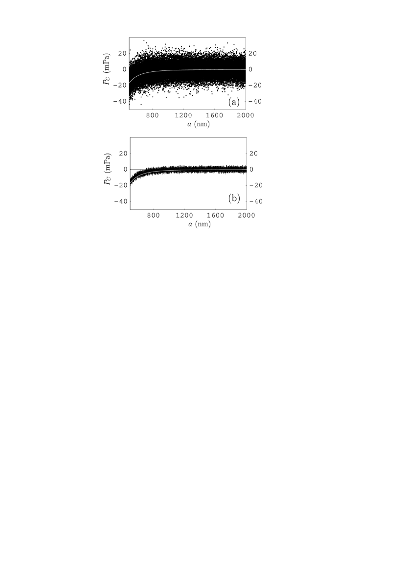
Figure 8: Comparison between (a) the individual and (b) mean experimental data for the Casimir pressure at $T=77\,$K (dots and crosses, respectively) and the common theoretical prediction of the Drude and plasma model approaches at $T=77\,$K (white lines).

To get an idea on the comparison between experiment and theory at larger separation distances, in Fig. 8 we show the theoretical predictions for the Casimir pressure at $T=77\,$K within the region from 500 to 2000 nm by the white bands (for the scale used the difference between the predictions of both approaches is again below the resolution). The results of all individual pressure measurements are indicated as dots in Fig. 8(a), whereas mean Casimir pressures with their total experimental errors are shown as crosses in Fig. 8(b). As can be seen in Fig. 8(a,b), the data are meaningful up to approximately 700 nm and at $a>1\,\mu$m the measured signal is averaged to zero. Thus, there is no offset in the calibration of our setup.

IV Conclusions and discussion

In the foregoing we have presented the measurement results for the normalized gradient of the Casimir force at liquid nitrogen temperature between Au-coated surfaces of a sphere and a plate. Using the PFA, these results were recalculated into the Casimir pressure between two Au-coated plates and compared with theoretical predictions of the Drude and plasma model approaches at $T=77\,$K and with the Casimir pressure measured at $T=300\,$K. It was found that although measurements at cryogenic temperatures are burdened with a larger systematic error, they are in a very good agreement with the measurement results at $T=300\,$K and with theoretical predictions of both approaches at $T=77\,$K. We have calculated the differences between the predictions of the Drude and plasma model approaches at $T=77\,$K and shown that they are below the instrumental sensitivity. We have also traced that with the increase of temperature up to $T=300\,$K the difference between the predictions of both approaches exceeds the increased instrumental sensitivity, so that the measurement data exclude the Drude model approach and are consistent with the plasma model approach.

The performed cryogenic measurements have been possible due to the use of dymanic AFM which can operate in high vacuum environments and temperatures between 5 K and 300 K. This setup opens prospective opportunities for measuring the Casimir interaction between different samples at variable temperature and for comparison of the obtained measurement data with theory. As is shown in this paper, there are no detectable changes in the thermal Casimir pressure when the measurement data taken at $T=77\,$K and $T=300\,$K are compared.

The obtained results shed some additional light on the possible role of surface patches in the comparison between measured and calculated Casimir pressures.39 As mentioned in Sec. I, measurements of the Casimir interaction between magnetic surfaces16 ; 40 are not compatible with this hypothesis. Under some assumptions a similar conclusion that there is no significant contribution of patches can be arrived for nonmagnetic (Au) surfaces when the measurement data at two different temperatures are compared. To see this, let us assume for a while that at $T=300\,$K there is large contribution of patch potentials to the measured pressure equal to $|P_{\rm patch}|=|P_{p}^{\rm th}(T=300\,\mbox{K})-P_{D}^{\rm th}(T=300\,\mbox{K})|\approx 9.36\,\mbox{mPa}>\Delta^{\!\rm tot}\bar{P}_{C}^{\rm expt}(T=300\,\mbox{K})=1.9\,$mPa at $a=235\,$nm (see Sec. III), such that ${P}_{D}^{\rm th}(T=300\,\mbox{K})+P_{\rm patch}\approx\bar{P}^{\rm expt}(T=300\,\mbox{K})$. This, however, comes into conflict with the fact that at $T=77\,$K our measurement data are in a good agreement with theoretical predictions of both the Drude and the plasma model approaches, which are very close: $P_{D}^{\rm th}(T=77\,\mbox{K})-P_{p}^{\rm th}(T=77\,\mbox{K})\approx 1.63\,\mbox{mPa}<\Delta^{\!\rm tot}\bar{P}_{C}^{\rm expt}(T=77\,\mbox{K})=4.4\,$mPa (see Sec. III). Really, if one would add the patch effect of –9.36 mPa to $P_{D}^{\rm th}(T=77\,\mbox{K})$, the obtained result of –295.9 mPa differs from $\bar{P}_{C}^{\rm expt}(T=77\,\mbox{K})=-287.9\,$mPa by 8 mPa, i.e., larger than the total experimental error determined at a 67% confidence level. Thus, under the assumption that the patch effect does not depend on temperature (i.e., it is the same at $T=300\,$K and $T=77\,$K) the presence of a large patch effect brings the experimental data at $T=77\,$K in disagreement with both the Drude and plasma model approaches to the Casimir force (the possibility of temperature-dependent patch potentials awaits further investigation).

To conclude, we express a hope that the fundamental understanding of the thermal Casimir interaction between real material bodies will be achieved in the near future.

                          

                          

                          

                          

                          

                          

Figure 6: The mean Casimir pressures previously measured at $T=300\,$K (a) by means of dynamic AFM15 and (b) by means of micromachined oscillator25 ; 26 are shown by the solid lines as functions of separation. The mean Casimir pressures measured in this work at $T=77\,$K with their total experimental errors determined at a 67% confidence level are indicated as crosses.

References

- (1) M. Kardar and R. Golestanian, Rev. Mod. Phys. 71, 1233 (1999).
- (2) R. H. French, V. A. Parsegian, R. Podgornik, et al., Rev. Mod. Phys. 82, 1887 (2010).
- (3) H. B. G. Casimir, Proc. K. Ned. Akad. Wet. B 51, 793 (1948).
- (4) E. M. Lifshitz and L. P. Pitaevskii, Statistical Physics, Part II (Pergamon, Oxford, 1980).
- (5) T. Emig, N. Graham, R. L. Jaffe, and M. Kardar, Phys. Rev. Lett. 99, 170403 (2007).
- (6) O. Kenneth and I. Klich, Phys. Rev. B 78, 014103 (2008).
- (7) M. Bordag, G. L. Klimchitskaya, U. Mohideen, and V. M. Mostepanenko, Advances in the Casimir Effect (Oxford University Press, Oxford, 2009).
- (8) G. L. Klimchitskaya, U. Mohideen, and V. M. Mostepanenko, Rev. Mod. Phys. 81, 1827 (2009).
- (9) G. L. Klimchitskaya, U. Mohideen, and V. M. Mostepanenko, Int. J. Mod. Phys. B 25, 171 (2011).
- (10) A. W. Rodriguez, F. Capasso, and S. G. Johnson, Nature Photon. 5, 211 (2011).
- (11) B. W. Harris, F. Chen, and U. Mohideen, Phys. Rev. A 62, 052109 (2000).
- (12) G. Bressi, G. Carugno, R. Onofrio, and G. Ruoso, Phys. Rev.Lett. 88, 041804 (2002).
- (13) R. S. Decca, D. López, E. Fischbach, G. L. Klimchitskaya, D. E. Krause, and V. M. Mostepanenko, Ann. Phys. (N.Y.) 318, 37 (2005).
- (14) G. Jourdan. A. Lambrecht, F. Comin, and J. Chevrier, Europhys. Lett. 85, 31001 (2009).
- (15) C.-C. Chang, A. A. Banishev, R. Castillo-Garza, G. L. Klimchitskaya, V. M. Mostepanenko, and U. Mohideen, Phys. Rev. B 85, 165443 (2012).
- (16) A. A. Banishev, G. L. Klimchitskaya, V. M. Mostepanenko, and U. Mohideen, Phys. Rev. Lett. 110, 137401 (2013).
- (17) F. Chen, U. Mohideen, G. L. Klimchitskaya, and V. M. Mostepanenko, Phys. Rev. A 74, 022103 (2006).
- (18) F. Chen, G. L. Klimchitskaya, V. M. Mostepanenko, and U. Mohideen, Phys. Rev. B 76, 035338 (2007).
- (19) S. de Man, K. Heeck, R. J. Wijngaarden, and D. Iannuzzi, Phys. Rev. Lett. 103, 040402 (2009).
- (20) S. de Man, K. Heeck, and D. Iannuzzi, Phys. Rev. A 79, 024102 (2009).
- (21) H. B. Chan, Y. Bao, J. Zou, R. A. Cirelli, F. Klemens, W. M. Mansfield and C. S. Pai, Phys. Rev. Lett. 101, 030401 (2008).
- (22) Y. Bao, R. Guérout, J. Lussange, A. Lambrecht, R. A. Cirelli, F. Klemens, W. M. Mansfield, C. S. Pai, and H. B. Chan, Phys. Rev. Lett. 105, 250402 (2010).
- (23) C.-C. Chang, A. A. Banishev, G. L. Klimchitskaya, V. M. Mostepanenko, and U. Mohideen, Phys. Rev. Lett. 107, 090403 (2011).
- (24) A. A. Banishev, C.-C. Chang, R. Castillo-Garza, G. L. Klimchitskaya, V. M. Mostepanenko, and U. Mohideen, Phys. Rev. B 85, 045436 (2012).
- (25) R. S. Decca, D. López, E. Fischbach, G. L. Klimchitskaya, D. E. Krause, and V. M. Mostepanenko, Phys. Rev. D 75, 077101 (2007).
- (26) R. S. Decca, D. López, E. Fischbach, G. L. Klimchitskaya, D. E. Krause, and V. M. Mostepanenko, Eur. Phys. J. C 51, 963 (2007).
- (27) A. O. Sushkov, W. J. Kim, D. A. R. Dalvit, and S. K. Lamoreaux, Nature Phys. 7, 230 (2011).
- (28) D. Garcia-Sanchez, K. Y. Fong, H. Bhaskaran, S. Lamoreaux, and H. X. Tang, Phys. Rev. Lett. 109, 027202 (2012).
- (29) V. B. Bezerra, G. L. Klimchitskaya, U. Mohideen, V. M. Mostepanenko, and C. Romero, Phys. Rev. B 83, 075417 (2011).
- (30) G. L. Klimchitskaya, M. Bordag, E. Fischbach, D. E. Krause, and V. M. Mostepanenko, Int. J. Mod. Phys. A 26, 3918 (2011).
- (31) G. L. Klimchitskaya, M. Bordag, and V. M. Mostepanenko, Int. J. Mod. Phys. A 27, 1260012 (2012).
- (32) M. Bordag, G. L. Klimchitskaya, and V. M. Mostepanenko, Phys. Rev. Lett. 109, 199701 (2012).
- (33) V. B. Bezerra, G. L. Klimchitskaya, V. M. Mostepanenko, and C. Romero, Phys. Rev. A 69, 022119 (2004).
- (34) B. Geyer, G. L. Klimchitskaya, and V. M. Mostepanenko, Phys. Rev. D 72, 085009 (2005).
- (35) K. A. Milton, J. Phys. A: Math. Gen. 37, R209 (2004).
- (36) I. Brevik, J. B. Aarseth, J. S. Høye, and K. A. Milton, Phys. Rev. E 71, 056101 (2005).
- (37) V. B. Bezerra, R. S. Decca, E. Fischbach, B. Geyer, G. L. Klimchitskaya, D. E. Krause, D. López, V. M. Mostepanenko, and C. Romero, Phys. Rev. E 73, 028101 (2006).
- (38) V. M. Mostepanenko and G. L. Klimchitskaya, Int. J. Mod. Phys. A 25, 2302 (2010).
- (39) R. O. Behunin, F. Intravaia, D. A. R. Dalvit, P. A. Maia Neto, and S. Reynaud, Phys. Rev. A 85, 012504 (2012).
- (40) A. A. Banishev, C.-C. Chang, G. L. Klimchitskaya, V. M. Mostepanenko, and U. Mohideen, Phys. Rev. B 85, 195422 (2012).
- (41) F. Chen, G. L. Klimchitskaya, V. M. Mostepanenko, and U. Mohideen, Phys. Rev. Lett. 90, 160404 (2003).
- (42) R. S. Decca, D. López, and E. Osquiguil, Int. J. Mod. Phys. A 25, 2223 (2010).
- (43) C. D. Fosco, F. C. Lombardo, and F. D. Mazzitelli, Phys. Rev. D 84, 105031 (2011).
- (44) G. Bimonte, T. Emig, R. L. Jaffe, and M. Kardar, Europhys. Lett. 97, 50001 (2012).
- (45) G. Bimonte, T. Emig, and M. Kardar, Appl. Phys. Lett. 100, 074110 (2012).
- (46) L. P. Teo, arXiv:1303.5176v1.
- (47) J. Laurent, H. Sellier, A. Mosset, S. Huant, and J. Chevrier, Phys. Rev. B 85, 035426 (2012).
- (48) R. Castillo-Garza and U. Mohideen, Rev. Sci. Instrum. 84, 025110 (2013).
- (49) H.-C. Chiu, C.-C. Chang, R. Castillo-Garza, F. Chen, and U. Mohideen, J. Phys. A 41, 164022 (2008).
- (50) F. J. Giessibl, Rev. Mod. Phys. 75, 949 (2003).
- (51) Handbook of Optical Constants of Solids, ed. E. D. Palik (Academic, New York, 1985).
- (52) A. Lambrecht and S. Reynaud, Eur. Phys. J. D 8, 309 (2000).
- (53) G. Bimonte, Phys. Rev. A 83, 042109 (2011).