Survival of interstellar molecules to prestellar dense core collapse and early phases of disk formation

Abstract

An outstanding question of astrobiology is the link between the chemical composition of planets, comets, and other solar system bodies and the molecules formed in the interstellar medium. Understanding the chemical and physical evolution of the matter leading to the formation of protoplanetary disks is an important step for this. We provide some new clues to this long-standing problem using three-dimensional chemical simulations of the early phases of disk formation: we interfaced the full gas-grain chemical model Nautilus with the radiation-magnetohydrodynamic model RAMSES, for different configurations and intensities of magnetic field. Our results show that the chemical content (gas and ices) is globally conserved during the collapsing process, from the parent molecular cloud to the young disk surrounding the first Larson core. A qualitative comparison with cometary composition suggests that comets are constituted of different phases, some molecules being direct tracers of interstellar chemistry, while others, including complex molecules, seem to have been formed in disks, where higher densities and temperatures allow for an active grain surface chemistry. The latter phase, and its connection with the formation of the first Larson core, remains to be modeled.

1. Introduction

Low mass stars like our Sun are formed by the collapse of a prestellar dense core. The matter falls in the center of the core, creating a protoplanetary disk surrounding a protostar. Planets, comets and other planetary/circumstellar bodies can then be formed in the disk. The chemical composition of the interstellar matter and its evolution during the formation of the disk are important to better understand the formation process of these planets and other bodies. In order to study the chemical evolution during the early phases of Solar System formation, one needs to know the evolution of the density and the temperature of the matter during the collapse process. Indeed, the chemical composition and its evolution depend mostly on these quantities. Besides, the chemical evolution is a non-equilibrium process, and thus it is necessary to follow the different phases of the collapse and disk formation to correctly deal with this subject.

The first phases are the following ones. After the beginning of the collapse, a first hydrostatic core at equilibrium is reached (when the density exceeds $10^{-13}$ g.cm^-3), which is called the first Larson core (Larson, 1969). This is the first step to the formation of the star and disk system. The accretion on the core continues, and when H₂ is dissociated (at a temperature of 2000 K), a second collapse begins, which leads to the formation of the second Larson core (when the density exceeds 1 g.cm^-3). The second Larson core is the protostar. First Larson cores have not been observed yet, mainly because they are embedded (high optical thickness) and have a short lifetime ($\sim 1000$ yrs). A few first candidates have been reported in recent years (Belloche et al., 2006; Chen et al., 2010; Enoch et al., 2010; Dunham et al., 2011; Pineda et al., 2011; Chen et al., 2012; Pezzuto et al., 2012) but their confirmation remains controversial since the expected observable signatures of first hydrostatic cores are still uncertain. However, recent progress has been made to characterize dust emission of first Larson cores (Commerçon et al., 2012).

To understand the link between the chemical composition of the interstellar medium and the one observed in disks, comets and other Solar System bodies, the chemical evolution of the matter needs to be coupled to the physics of the prestellar collapse. The chemistry of collapsing cores has been studied using one-dimensional models (Ceccarelli et al., 1996; Rodgers & Charnley, 2003; Doty et al., 2004; Lee et al., 2004; Garrod & Herbst, 2006; Aikawa et al., 2008; Garrod et al., 2008). van Weeren et al. (2009) and Visser et al. (2011) presented two-dimensional chemical evolution during the collapse of a molecular cloud to form a low-mass protostar and its surrounding disk. As a first step to study the detailed coupling between the dynamics of the formation of disks and their chemical composition, Furuya et al. (2012) (hereafter FA12) performed three dimensional radiation-hydrodynamical simulations of star formation coupled with a detailed chemical network.

To go a step further, we present in this paper three-dimensional chemical simulations of the early formation of a primitive protoplanetary disk using a radiation-magneto-hydrodynamic model, where the magnetic field allows for the formation of more realistic disks, less prone to early fragmentation (Commerçon et al., 2011). We have computed the evolution of the chemical composition of gas and ices using a full gas-grain chemical network, in a collapsing prestellar dense core up to the first Larson core (just before the onset of the second collapse). The core physical structure has been consistently derived using state-of-the-art radiation-magneto-hydrodynamic (RMHD) models of star formation. From these simulations, we infer how the chemical composition of the initial parent cloud is modified by the formation of the disk.

The paper is organized as follows. In section 2, the chemical and physical models are presented. The results are then shown and discussed respectively in sections 3 and 4.

2. Model

For this modeling, we have used the gas-grain chemical code Nautilus (Hersant et al., 2009) with the physical conditions of a collapsing dense core computed using the adaptive mesh refinement code RAMSES (Teyssier, 2002).

2.1. The physical model RAMSES

The physical structure of the collapsing core is derived using the RMHD solver of RAMSES which integrates the equations of ideal magnetohydrodynamics (Fromang et al., 2006) and the equations of radiation-hydrodynamics under the grey flux-limited diffusion (FLD) approximation (Commerçon et al., 2011a). The initial conditions are those used in Commerçon et al. (2012) and consist in a 1 M_⊙ sphere of uniform density $\rho_{0}=3.97\times 10^{-18}$ g.cm^-3 (corresponding to a molecular hydrogen number density $n_{\rm H_{2}}\approx~{}10^{6}$ cm^-3) and temperature $T_{0}=11$ K. The sphere (radius $r_{0}\approx 3300$ AU) is in solid body rotation, and threaded by a uniform magnetic field. The strength of the magnetic field is expressed in terms of the mass-to-flux to critical mass-to-flux ratio $\mu=(M_{0}/\Phi)/(M_{0}/\Phi)_{\mathrm{c}}$. $M_{0}$ is equal to M_⊙. $\Phi$ is the magnetic flux. If $(M_{0}/\Phi)$ is lower than $(M_{0}/\Phi)_{\mathrm{c}}$ (i.e. $\mu$ is lower than 1), then the core is supported against its own gravity by the magnetic field, and does not collapse. In this study, we use two magnetization levels: a moderate one ($\mu=10$) and a low one ($\mu=200$). For $\mu=10$, we use two different initial configurations: an angle $\Theta=0\degree$ between magnetic field lines and the rotation axis of the sphere, and an other angle $\Theta=45\degree$. These values form three different models that we present in this paper: MU10$\Theta$0, MU10$\Theta$45 and MU200$\Theta$0 (see Table 1). We computed the evolution of the collapsing dense core throughout the first collapse and first Larson core lifetime (Larson, 1969), i.e. $\sim 38\times 10^{3}$ yr. The RMHD method used in RAMSES has been well tested, as well as the numerical convergence by Commerçon et al. (2010). Accordingly, the grid is dynamically refined as a function of the local Jeans length so that it is always resolved by at least 10 cells. In addition, it has been shown in previous studies that the grey FLD approximation is well adapted to study the early phases of star formation by comparing to more advanced moment and multifrequency models (Commerçon et al., 2011b; Vaytet et al., 2012).

Table 1Magnetic fields strength and orientations used for the current simulations.

Model	$\mu$	$\Theta$ (°)
MU10$\Theta$0	10 (moderate)	0
MU10$\Theta$45	10 (moderate)	45
MU200$\Theta$0	200 (low)	0

2.2. The chemical model Nautilus

Nautilus computes the abundance of species in the gas-phase and at the surface of the grains as a function of time, taking into account pure gas-phase chemistry (bimolecular reactions, dissociative and radiative recombinations and associations, electron attachments, dissociations and ionizations induced by cosmic-rays and UV photons…), interaction between the species in the gas-phase and the grain surfaces (adsorption, thermal desorption, and non-thermal desorption by cosmic-rays), and grain surface reactions (chemical reactions, and dissociation by UV photons and cosmic ray induced photons). A more detailed description of this model and the chemical network can be found in Semenov et al. (2010), and Hincelin et al. (2011). The network has been updated according to the latest recommendations from the KIDA experts until October 2011. An electronic version of our network is available at http://kida.obs.u-bordeaux1.fr/models.

To compute the initial chemical composition of the sphere, we run Nautilus for dense cloud conditions (10 K, H density of $2\times 10^{5}$ cm^-3, cosmic-ray ionization rate of $1.3\times 10^{-17}$ s^-1 and a visual extinction of 30) for a time $t\sim 6\times 10^{5}$ yr, assuming that species are initially in the atomic form except for hydrogen, which is already molecular. We used the elemental abundances from Hincelin et al. (2011), with an oxygen elemental abundance relative to total hydrogen equal to $1.5\times 10^{-4}$ (C/O ratio equal to $1.13$). For each element, we define the elemental abundance as the ratio of the number of nuclei both in the gas and on the dust grains to the total number of H nuclei. This excludes the nuclei locked in the refractory part of the grains, that is why we did not use solar elemental abundances which takes into account this refractory part. The chosen time $t$ corresponds to the maximum of agreement between observations of molecular clouds and our simulations (see Fig.3. of Hincelin et al. (2011)). Using this chemical composition as the initial condition, we then run the chemistry during the collapse using the method described in the next subsection.

2.3. Interface between Nautilus and RAMSES codes

To simplify our simulations, already very time consuming, there is no feedback of the chemical composition calculated by Nautilus on the dynamics computed using the RAMSES code, i.e. Nautilus computations are a post-processing of RAMSES simulations (see section 4.4). To compute the chemistry, Nautilus needs two input data: the temperature and the density as a function of time. For both the physical and chemical calculations, we assume that the object is embedded in a cloud so that direct photoprocesses can be neglected (visual extinction is fixed to 30) and that the cosmic-ray ionization rate is constant (fixed to $1.3\times 10^{-17}$ s^-1). The first step of the calculation is to obtain the time dependent physical conditions. To this aim, we introduce $10^{6}$ “probe” particles, initially uniformly distributed in the sphere, which handle the temperature, density and velocity history of the fluid through a Lagrangian approach. For any particle, at each time step, the position is registered, the temperature, density and velocity are extracted according to the local fluid properties, and the position at the next time step is iterated. At the end of this process, we obtain the positions, the velocities, and the couples temperature/density $\rm(T(t),n(t))$ as a function of time $t$ for the million particles of the model. Fig. 1 shows an example of computed trajectory and its corresponding $\rm(T(t),n(t))$. Starting from the initial chemical composition of the sphere, the chemical evolution is then computed in 0D for each parcel of material (“probe” particle) using the physical conditions derived from the RMHD simulations (i.e. the $10^{6}$ couples $\rm(T(t),n(t))$). Note that the chemistry does not have the time to reach steady state in any of our calculations. This process gives the full 3D chemical structure of the collapsing dense core as a function of time. Central Processing Unit (CPU) time to compute the chemical evolution of $10^{6}$ particles (i.e. for one model) is roughly $10^{4}$ hours (using JADE cluster from CINES).

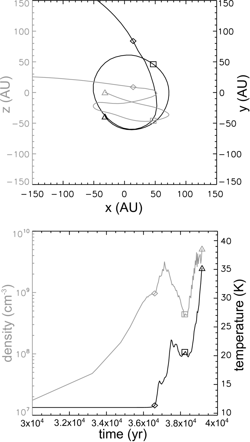
Figure 1.— Example of a trajectory in cartesian coordinate system (top) and the associated temperature T(t) and density n(t) as a function of time t (bottom), for one given particle of model MU10$\Theta$45. Diamond, square and triangle show positions (top) at specific times (bottom). The center of first Larson core has coordinates $\rm(x,y,z)=(0,0,0)$.

3. Results

3.1. Physical properties of disks

Within this structure, we identify several components representing 1) the core itself (the first Larson core), 2) the outflow, 3) the rotating disk, 4) the magnetically supported pseudodisk, and 5) the envelope, based on criteria from Joos et al. (2012). More details on the extraction method will be given in a future paper (Hincelin et al. in preparation). The rotating disk component that we consider here is made by particles that satisfy the four following criteria:

1. an azimuthal velocity $v_{\phi}$ more than two times larger than their radial velocity $v_{r}$,

2. an azimuthal velocity more than two times larger than their vertical velocity $v_{z}$,

3. a rotational support (density of rotational kinetic energy $E_{k}=0.5\rho v_{\phi}^{2}$, where $\rho$ is the mass density) at least two times larger than the thermal support (density of internal energy $E_{i}=1/(\gamma-1)\times(\rho k_{B}T)/(\mu_{m}m_{\rm H})$, where $\gamma$, $k_{B}$, $\mu_{m}$, and $m_{\rm H}$ are respectively the adiabatic index, the Boltzmann constant, the mean molecular weight, and the mass of hydrogen nucleus),

4. and a density above $10^{9}$ cm^-3.

Fig. 2 and 3 present selected particles that belong to the rotating disk for the three models presented in Table 1. The other components (central core, outflow, pseudodisk and envelope) will be discussed in a future paper (Hincelin et al. in preparation). The plotted information (in color) are respectively the temperature and the density of the particles. The disks are relatively cold, around 10 K, except at low radius where the temperature can reach about 100-200 K. Density spreads from $10^{9}$ to $10^{11-12}$ cm^-3 from the outer edge of disks to their center. The temperature profile has roughly a spherical symmetry (except for model MU200$\Theta$0 with the presence of four ”hot spots” around the central core) which is due to the central core (see also Fig.2 in Commerçon et al. (2012)), while the density profile has a more complex shape, for example with the presence of spiral arms for $\mu=10$ (MU10$\Theta$0 and MU10$\Theta$45 models). In these simulations, the disk of model MU10$\Theta$0 is about 200 AU in diameter, whereas the one of model MU10$\Theta$45 is roughly two times larger ($\sim 400$ AU). Due to the low magnetization level, the disk of model MU200$\Theta$0 shows a more complex shape with fragmentation. Four “hot spots” are identified around a central disk. Each spot is characterized by an increase of both temperature and density. The central disk is about 80 A.U. in diameter. Table 2 shows the range of sizes, temperatures and densities found in the disks at the end of simulations for the three models. One notes that the disk of model MU200$\Theta$0 is fragmented due to the low magnetization level, and the disk of model MU10$\Theta$45 is twisted because of the inclination between rotational axes and initial magnetic field lines.

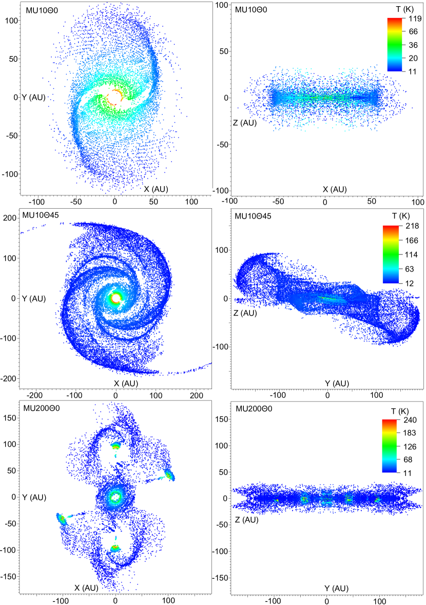
Figure 2.— Temperature (K) in the disk for the three models MU10$\Theta$0, MU10$\Theta$45 and MU200$\Theta$0. Face-on view on the left and edge-on view on the right. Particles are projected in the plane (xOy), (xOz) or (yOz). The color coding is linear.

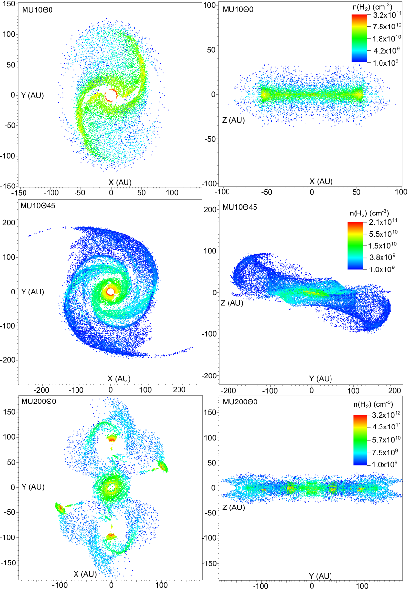
Figure 3.— Density of H₂ (cm^-3) in the disk for the three models MU10$\Theta$0, MU10$\Theta$45 and MU200$\Theta$0. Face-on view on the left and edge-on view on the right. Particles are projected in the plane (xOy), (xOz) or (yOz). The color coding is logarithmic.

Table 2Size (diameter and thickness), temperature and density ranges in the disks for models MU10$\Theta$0, MU10$\Theta$45 and MU200$\Theta$0 at the end of simulations.

Model	Diameter (AU)	Thickness (AU)	Temperature (K)	Density (cm-3)	Final time (yr)
			min. - max.	min. - max.
MU10$\Theta$0	$\sim$ 200	60	11 - 119	1(9) - 3(11)	$3.7\times 10^{4}$
MU10$\Theta$45	400	100	12 - 217	1(9) - 2(11)	$3.9\times 10^{4}$
MU200$\Theta$0	80	40	11 - 160	1(9) - 3(12)	$3.9\times 10^{4}$

3.2. Chemical composition of the disks for the three physical models

3.2.1 Chemical evolution of the matter from the cloud to the disk

Fig. 4 shows the sum of the abundances computed in the gas phase and at the surface of the grains (ices) compared to the total hydrogen (proton) density for a selection of species, at two different steps of the simulations: 1) the initial condition, i.e. the composition of the parent molecular cloud, before the beginning of the collapse (namely the sphere in section 2.2 and 2.3), and 2) the final condition, i.e. the composition in the disk. A change in this total abundance compared to the chemical content of the cloud implies that some processes of formation or destruction have occurred during the collapse in addition to just adsorption and desorption processes. As the modeled object is embedded in a dense envelope, the effects of ionization and dissociation by the external UV photons are low compared to bimolecular chemical reactions. The main result of our simulations is that the chemical content is unchanged during the collapse: there is no significant evolution of the global (ice plus gas) abundances of the species. For example, the abundances of water (H₂O), methane (CH₄), carbon monoxyde (CO) and ammonia (NH₃) are the same in the parent cloud and the disk.
There are a few exceptions: HNC, CO₂ and HNO. HNC is very sensitive to the evolution of temperature and density during the collapse: in the case of model MU200$\Theta$0, its mean total abundance has decreased from about $5\times 10^{-7}$ (cloud composition) to $4\times 10^{-9}$ (disk composition), i.e. two orders of magnitude. The matter close to the fragments is hot so that HNC desorbs from grain and is efficiently destroyed in the gas phase by $\rm H_{2}COH^{+}+HNC\longrightarrow HCNH^{+}+H_{2}CO^{(}$⁾. Then the HCN/HNC ratio (taking into account gas and ices) can exceed 100. One notes on Fig. 4 that, even during the cloud stage, the ratio HCN/HNC is not equal to 1, but roughly equal to 10. While the gas phase ratio is equal to 1, HCN and HNC abundances are higher on grain surfaces than in the gas phase, so that the grain surface ratio leads to a total ratio (gas and ices) of 10. On the grain surface, HCN and HNC are photodissociated into CN and H. Then, CN and H react on the surface, but form preferentially HCN and not HNC. HNC can be formed on the surface using different pathways (C + NH, C + NH₂ or CH + NH), but these reactions are less efficient than $\rm CN+H\longrightarrow HCN$ so that the ratio HCN/HNC on grain surfaces reaches a value of 10. One notes that as a consequence, desorption of ices could enhance the gas phase ratio HCN/HNC to a value of 10. On the contrary but to a lesser extent, the mean global abundance of CO₂ has increased from the cloud to the disk, by a factor of two in the model MU10$\Theta$45. High temperature promotes CO₂ formation on the grain surface, particularly through $\rm OH+CO\longrightarrow CO_{2}+H$ (Ruffle & Herbst, 2001). Desorption of HNO ices is followed by gas-phase reactions mainly involving CH₃, O, CH₂, and CN, that produce NO and respectively CH₄, OH, CH₃ and HCN.

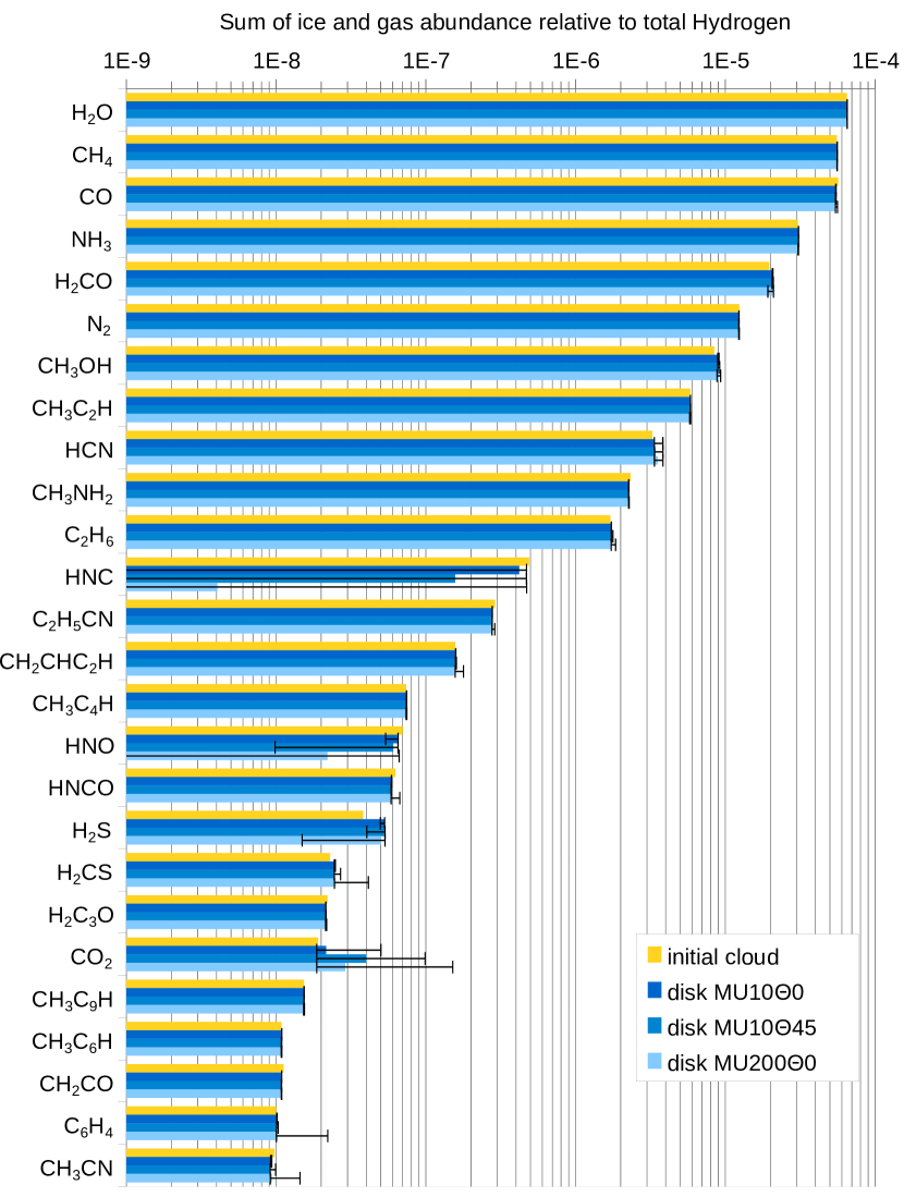
Figure 4.— Abundance (in the ices and in the gas-phase) relative to total hydrogen of the most abundant species (with an abundance more than $\simeq 10^{-8}$), in the initial cloud (yellow), and in the rotating disk at the end of the simulations for the three different models: MU10$\Theta$0 (dark blue), MU10$\Theta$45 (blue) and MU200$\Theta$0 (light blue). The plotted values for disks are the logarithm of abundance, averaged on the number of selected particles that belong to the disk. The line segments show minimum and maximum values of species abundances.

3.2.2 Ice composition in the disk of model MU10$\Theta$0

To illustrate the chemical composition of the ices in the disks, we present in this section the distribution of the ice composition for model MU10$\Theta$0 and for a selection of molecules observed in comets. Fig. 5 shows the maximum (in blue) and minimum (in black) relative abundances compared to H₂O on the grain surfaces for these species together with the abundances observed in comets. Abundances below $10^{-3}$% are not shown. In some cases, the abundances are constant, like for NH₃ so that the minimum overlaps the maximum and only black is seen. On the contrary, if the species abundance shows a gradient in the disk and that the smallest abundance is below $10^{-3}$, only the maximum value, in blue, appears in Fig. 5. As an example, the abundance of methanol ice (CH₃OH) compared to water ice is about 14 % all over the radius of the disk (in the figure, the black band (minimum) overlays the blue one (maximum)). The abundance of carbon monoxyde ice (CO) is high from the outer edge of the disk to around 30 AU from the central first Larson core (the blue band reaches 84 %). Within this radius, the CO desorbs from the grain and the ice abundance falls down to $10^{-11}$ % (this value, being under 0.001 %, is not visible in Fig. 5). The abundance of formic acid ice (HCOOH) is low ($2\times 10^{-4}$ %) all over the radius of the disk, which is below our 0.001 % threshold, hence not visible in Fig. 5).

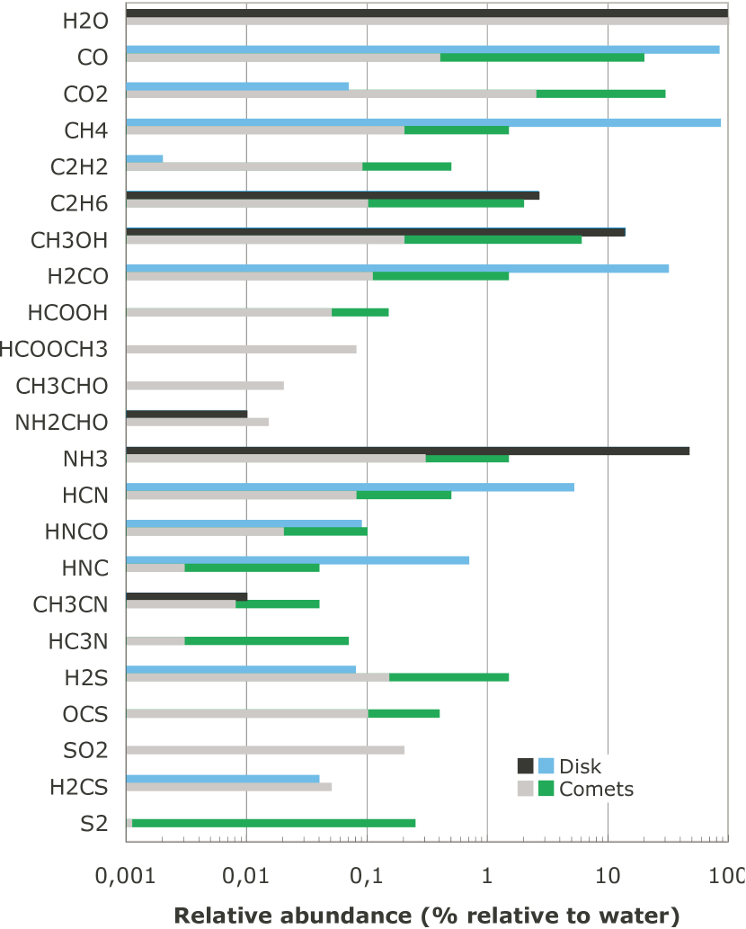
Figure 5.— Abundances of species in the ices relative to water on the grain surface. The maximum and minimum computed values in the disk of model MU10$\Theta$0 are respectively shown in blue and black. The range of measured values in comets is shown in the green portions; in this case the gray indicates the minimum; if species have been observed only once, there is no green portion (from Mumma & Charnley (2011)). The abundance of water on grain surfaces relative to total hydrogen is $6.5\times 10^{-5}$.

Species listed in Fig. 5 can be divided in three groups (Table 3). The first group contains molecules with nearly uniform abundances as a function of the radius (such as water ice because of its relatively high evaporation temperature). In the second group, molecules are more abundant on ices in the outer ($>$25 AU), cold ($\sim$25 K) disk (such as CO ice), while the reverse is true for molecules in the third group (such as C₂H₂). The reason for the abundance decrease in the inner parts for the second group is evaporation due to higher temperatures. In that case, the gas phase abundance essentially reflects the initial content of the ices, with mainly one exception, HNC, which is quickly destroyed by gas-phase reactions (see section 3.2.1) when the temperature is larger than $\sim$50 K (within a radius of $\sim$12 AU from the center).

Table 3Groups of molecules on grain surfaces according to their behavior in the disk for model MU10$\Theta$0.

Homogeneous	H2O, C2H6, CH3OH, HCOOH,
	NH2CHO, NH3, CH3CN
Outer disk	CH4, H2CO, HCN, HNCO, H2CS, HNC,
	H2S, CO, CH3CHO, S2, CO2
Inner disk	C2H2, HCOOCH3,HC3N, OCS, SO2

The projected H₂O_(ice), CO_(ice) and C₂H_2(ice) abundances (relative to total hydrogen) computed in the disk for the model MU10$\Theta$0 are shown in Fig. 6. These three molecules illustrate the different behaviors presented in Table 3. The temperature is rather low, below 20 K in the majority of the disk (from the outer edge to $\sim$40 AU) whereas the total H density presents variations between $10^{9}$ and $8\times 10^{10}$ cm^-3 from the outer edge to $\sim$15 AU. The inner regions (within a radius $r\approx 20$ AU) present the warmest part of the disk with temperatures up to about 120 K. The abundance of water (relative to total hydrogen) trapped on interstellar grains is constant across the disk at a value of $6.5\times 10^{-5}$. The decrease of the CO ice abundance is a direct consequence of thermal evaporation in this region. When the temperature increases (as a function of the radius), electronic recombination reactions in the gas phase enhance the abundance of C₂H₂. The gas-phase C₂H₂ is then adsorbed on grains. Desorption is not efficient for this species because its adsorption energy is high enough.

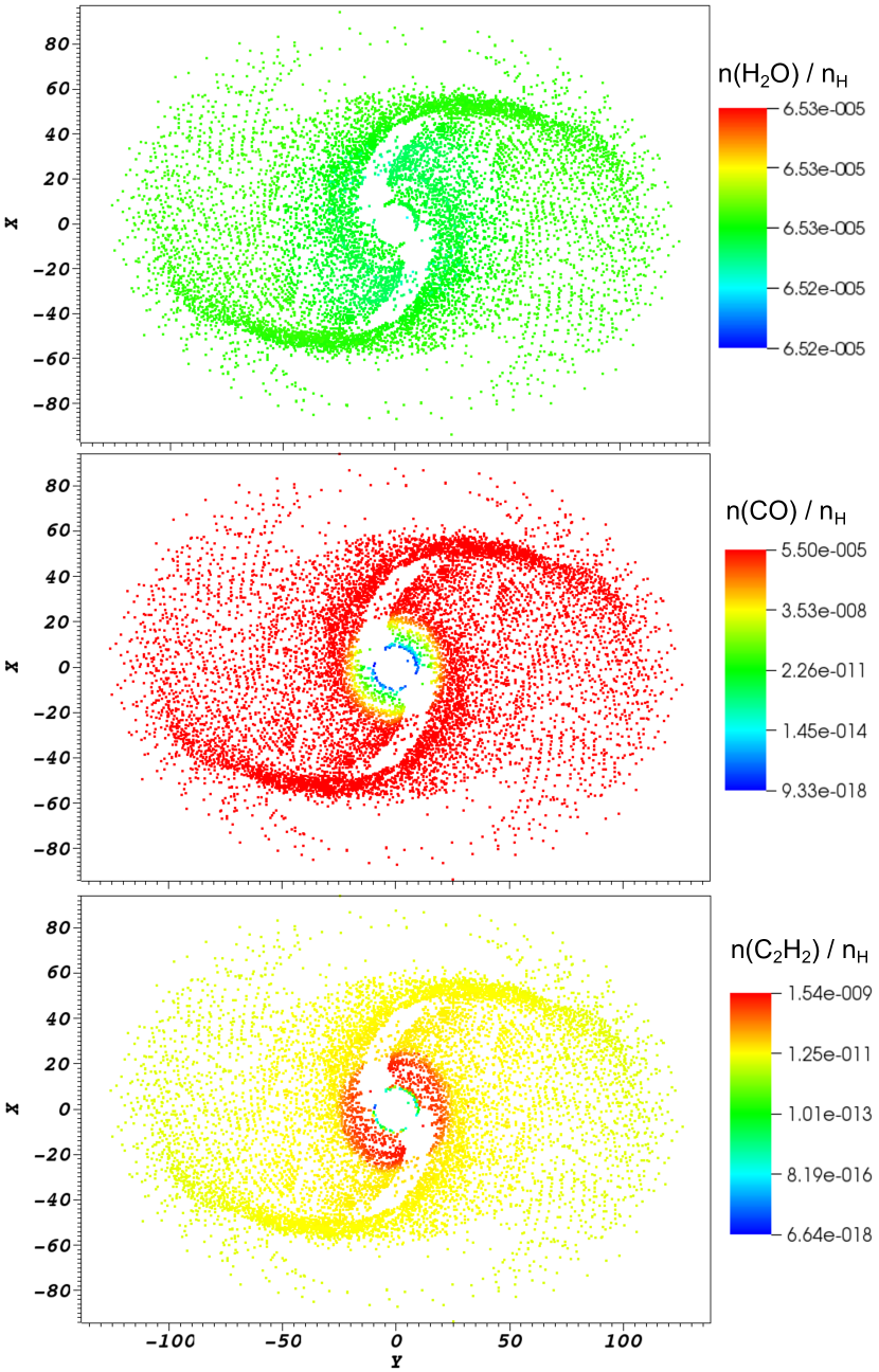
Figure 6.— H₂O, CO and C₂H₂ abundances relative to total H in the ices in the rotating disk of model MU10$\Theta$0. The ”central and spiral hole pattern” is composed of particles that do not respect the criteria of a disk according to Joos et al. (2012) (i. e. belong to the core or are not supported by rotation).

Results for model MU10$\Theta$45 and MU200$\Theta$0 are qualitatively similar to those of MU10$\Theta$0, with some different distributions of molecules according to the local temperature and density conditions. Due to fragmentation and the presence of four hot spots in the model MU200$\Theta$0, ices are sublimated in these hotter regions, and molecules are eventually destroyed in the gas phase. The higher temperature of the matter next to these regions lead to a more active surface chemistry which enhances the formation of complex organic molecules such as the methylformate $\rm HCOOCH_{3}$. The disk of the model MU10$\Theta$45 is on average a little bit warmer, which leads to a smaller abundance of ices but a higher abundance in the gas phase so that the total abundance is globally not changed in a significant amount (see Fig.4).

4. Discussion

4.1. Comparison with comets

Our model stops just before the second collapse and the formation of the second Larson core, which is early in the star formation process (see section 4.4). However, recent hydrodynamic simulations (Machida et al., 2010; Machida & Matsumoto, 2011; Bate, 2010, 2011) have shown that the central part (radius $\lesssim 1$ AU) of the first Larson core will form the second Larson core, that is to say the protostar, whereas the outer part of the first Larson core will evolve in a disk. During the protostellar phase, a small fraction of the first core material should have been transported to the outer region of the disk, and not been accreted to the protostar (see discussion of FA12).
Considering the partial interstellar origin of the molecules observed in comets (Bockelée-Morvan et al., 2000; Mumma & Charnley, 2011), it is then interesting to compare the comet chemical composition and the results of our models. Due to the fact that our disk is very young, the computed ice can be considered as ”pre-cometary”, and so this comparison must stay qualitative.

The ice abundances of C₂H₆, CH₃OH, NH₂CHO and CH₃CN found in our disk for model MU10$\Theta$0 are within a factor of 2 of those found in comets (see Fig. 5). It is also the case for HNCO, H₂S and H₂CS in the outer part of the disk where the temperature is low enough to maintain these species on grain surface. These species represent about one third of the observed species in comets. On the other hand, CO₂, C₂H₂, HCOOH, HCOOCH₃, CH₃CHO, HC₃N, OCS, SO₂ and S₂ are strongly underproduced in our model, in the entire disk, compared to comets. Carbon dioxide (CO₂) and carbon sulfide (OCS) are known to be abundant on interstellar ices (Palumbo et al., 1997; Gibb et al., 2000) but not much produced by astrochemical models at low temperature because carbon, oxygen and sulfur only diffuse slowly on surfaces (Ruffle & Herbst, 2001). For example, the surface reaction $\rm HCO+O\longrightarrow CO_{2}+H$ is the main pathway in our model for CO₂ production, but is in competition with $\rm HCO+H\longrightarrow H_{2}CO$ which is faster. In our results, CH₄ and NH₃ are reservoirs of carbon and nitrogen whereas they are minor species in comets. The methane is probably overproduced in our model because we underestimate the formation of CO₂: the available carbon on grain surfaces is quickly hydrogenated so the carbon is rather locked into methane. For nitrogen, the reservoir is not known in comets (Bockelée-Morvan et al., 2004) and we probably lack some mechanisms to form other N-bearing species (Daranlot et al., 2012). Finally, HCOOH, CH₃CHO and HCOOCH₃ are known to trace warmer regions where radicals can move at the surface of the grains, and are typically observed in warmer star forming regions (Herbst & van Dishoeck, 2009).

Comets seem to be made of molecules formed in different physical conditions. Table 4 illustrates this idea proposing a formation place of molecules where the required physical conditions are present. The HNC molecule for instance, is a strong signature of cold interstellar like-chemistry. Other molecules on the contrary, such as HCOOCH₃, require temperatures of about 40 to 60 K to be formed on surfaces (Garrod & Herbst, 2006), and as a consequence are not produced by our model in the disk in sufficient amount. This mixed composition may be a strong indication of radial mixing in the protoplanetary disk. This process is not included in our simulations. In fact, we find that the composition of ices are almost constant in the outer regions but that there is a gradient of abundances within 40 AU, a size consistent with the assumed region of formation of comets in our solar system (see Mumma & Charnley (2011) and references within it).

Table 4Possible formation place of molecules observed in comets.

Cloud	C2H6, CH3OH, HNCO,
(low temperature)	NH2CHO, CH3CN, H2S, H2CS
Cloud	CH4, H2CO, HCN,
+ desorption process	HNC, CO
Close to the first core	CO2, C2H2, CH3CHO, OCS,
(warmer region)	HCOOH, HCOOCH3

4.2. Impact of initial conditions on the survival of molecules during the collapse

In order to assess the sensitivity of our results to the composition of the initial dense core, we computed the chemical composition for three different particles of model MU10$\Theta$0 using several initial conditions. The three particles reach at the end of the simulation respectively the cold region ($\sim 10$ K), the warm region ($\sim 30$ K) and the hot region ($\sim 100$ K) of the disk.

4.2.1 A denser molecular cloud

As a first test, we constructed our initial conditions from a Nautilus run with a density of $2\times 10^{6}$ cm^-3, i.e. ten times higher than the one of our standard initial conditions described in section 2.2, for $6\times 10^{5}$ yr. The resulting dense core composition is in fact similar to the standard one. Differences mostly concern atoms, whose abundances are lowered by one to two orders of magnitude at the final time. However, the reservoirs of carbon, oxygen and nitrogen remain CO, CO₂, H₂O and NH₃ and their abundances are not changed significantly.
Consequently, the evolution of our three particles during the subsequent collapse keeps the properties described in section 3.2.1: the most abundant molecules fully survive, only trace species are altered, the most sensitive being HNC, with an abundance lowered by 6 orders of magnitude for the particle reaching the hot region of the disk.

4.2.2 An older molecular cloud

Knowing the large uncertainties pertaining to the age of molecular clouds (see for example Hartmann et al. (2001), Mouschovias et al. (2006), Ballesteros-Paredes & Hartmann (2007), and Pagani et al. (2011)), we constructed another set of initial conditions for the same physical parameters as for the standard one, but for an evolution during $6\times 10^{6}$ yr, i.e. ten times longer. The resulting composition is different in such a case. The most notable difference is that CO is no longer a carbon and oxygen reservoir. The abundance of CO in the cloud is decreased in favor of H₂O and CH₄: chemistry being out of equilibrium, the longer integration time allows adsorption of CO on the grain surface, which is followed by successive hydrogenation that leads to CH₃OH formation. Then, photodissociation of CH₃OH by cosmic ray induced UV photons produces CH₃ and OH, which are hydrogenated to form CH₄ and H₂O (see Garrod et al., 2007, for details about this process).
With such initial conditions, our main conclusions remain unchanged, only trace species are altered. Interestingly enough, CO is not a reservoir in this case and shows a significant evolution during the collapse, with an abundance decreasing by up to 3 orders of magnitude for the particle arriving in the warm region of the disk, because of adsorption followed by grain surface reactions. This effect is less strong for the other two particles: for the one arriving in the hot zone, CO desorbs sooner, while the one arriving in the outer parts sees lower temperatures, both effects making grain surface reactions less efficient.

4.2.3 Observed abundances in dense clouds as initial conditions

Another natural choice for the initial conditions is to use the composition actually observed in dense cores. The gas phase abundances were taken from observations of TMC-1(CP). The ice abundances of CO₂, CO, NH₃, CH₃OH, and OCS were taken from observation of Elias 16, a K1 giant behind TMC, considered as a quiescent environment (Gibb et al., 2004). The abundance of water ice is set to its median value observed in cold dense sources, which is about $5\times 10^{-5}$ relative to total hydrogen (Gibb et al., 2004; Pontoppidan et al., 2004; Boogert & Ehrenfreund, 2004; Öberg et al., 2011). To conserve the same elemental abundances as in the standard model, the atomic abundances have been adjusted.
The chemical evolution during the collapse is more significant in this case. Apart from the five most abundant molecules, CO, H₂O, CO₂, NH₃, and CH₃OH, who survive the collapse and remain reservoirs, most species see their abundances change during the collapse. This is due to the fact that the initial condition is not a quasi-stationary state for our chemical network, as our network does not reproduce exactly the observed abundances in dense clouds. Consequently, as soon as the calculation starts, rapid gas phase reactions tend to relax the system towards a chemical state more consistent with our chemical network and most abundances change.
However, it is worth noting that, even in this case, the most abundant species survive the collapse.

This study of the influence of initial conditions strengthens the conclusions of section 3.2.1: the memory of the composition of the prestellar core is kept throughout the first phases of the formation of the disk, at least for the most abundant species.

4.3. Comparison with other three-dimensional numerical simulations

FA12 present three-dimensional modeling results of a collapsing dense core until the formation of the first hydrostatic core, that is to say the first Larson core. They use a similar interface as ours: they use fluid particles that trace the physical conditions of the matter during the collapse, and compute the chemical evolution on these particles as a post-process. The main differences with our model are that FA12, on a physical point of view, do not compute the effect of magnetic field on the collapse process, and on a chemical point of view, use a high temperature gas-phase network (for a range of 100-800 K). Since we focus on the disk composition in the present paper, where the temperature does not exceed 300 K, we do not expect our results to be affected by this limitation (see section 4.4).

Figure 7 shows the density and temperature of particles in the equatorial plane (area where $|z|<10$ AU) as a function of the distance from the central core, for the model MU10$\Theta$0. At a given radius, the range of values come from the asymmetry of the collapsing core: in particularly, because of the presence of spiral arms. The figure can be compared to panel (b) of Figure 9 of FA12 (although the integration time is not exactly the same): the temperature and density profiles are qualitatively similar, except within 1-2 AU where the density and temperature are higher in the case of FA12. In our model, an additional support against gravitational collapse exists, magnetic support, which limits contraction. As a consequence, the inner computed temperature and density are lower in our case. One of the main conclusion of FA12 is that the total gas and ice abundances of many species remain unaltereted during the collapsing process until the temperature reaches about 500 K, that is to say at a spherical radius $r\lesssim 3$ AU. The gas phase abundances are determined via desorption process, depending on the adsorption energy of species on the surface of the grains. Our results show similar conclusion, at least for the disk component: except at low radius, the chemical composition is globally unaltered during the collapse with a gas phase abundances mainly determined by desorption. In the warmer parts of the disk, that is to say at lower radius, we also observe a formation of carbon chains and large organic molecules such as C₂H₂, HC₃N and HCOOCH₃ (see Table 3).

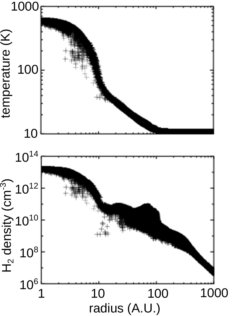
Figure 7.— Temperature and density of particles that belong to the equatorial plane (where $|z|<10$ AU) as a function of the radius at the end of the simulation for the model MU10$\Theta$0.

4.4. Limits of the model

The simulations from the RMHD physical model RAMSES stop just before the start of the second collapse. The formation of this second core increases the temperature in the disk at larger radii as suggested by the 1D modeling of Vaytet et al. (2013). Compared to our simulations, this may mainly change the radii at which molecules evaporate. The importance of this second phase will depend on the temperature gradient obtained in the disk. This issue will be investigated in further studies.

The physical model RAMSES integrates the equations of ideal magnetohydrodynamics, assuming the medium to be a perfect conductor. The matter is then frozen on the magnetic lines. If we consider a medium that is not a perfect conductor, that is to say in the case of non ideal (or resistive) magnetohydrodynamics, the neutral matter will be able to cross magnetic lines. This induces a friction between ions and neutrals, called ambipolar diffusion (Mestel & Spitzer, 1956; Mouschovias, 1991). Ambipolar diffusion generates a net velocity difference between ions and neutral that can be sufficient to overcome activation barriers, thereby generating efficent reaction pathways. Future work would be done to couple non ideal magnetohydrodynamics with chemistry in order to take this phenomenon into account. Recent works have been done to integrate ambipolar diffusion in RAMSES (Masson et al., 2012).

As mentioned in section 2.3, the chemical model Nautilus is used as a post-processing of the RAMSES computation. There is no chemical feedback on the physical structure of the collapsing dense core. But, a radiative cooling of the matter due to chemical species such as CO, CH₄, H₂O, C and O can occur. The cooling rate of a given chemical species depends in particular on the temperature and the density of the medium, and the abundance of the species (see for example Neufeld & Kaufman, 1993; Dedes et al., 2011). However, at high density such as in the case of our modeling, the cooling is mostly dominated by the radiative emission of the dust.

In our modeling, each particle is independent of the others from a chemical point of view. This is valid only if mixing effects can be neglected, both molecular diffusion and turbulent mixing.
For matter collapsing onto the core and the disk, our simulations do not show any turbulent motion, and in general turbulent mixing is not expected to be efficient during this phase. The influence of molecular diffusion can be qualitatively estimated by comparing the characteristic diffusion timescale $\tau_{\mathrm{diff}}$ for two nearby tracer particles, with the time $\tau_{\mathrm{disk}}$ for these particles to enter the disk. $\tau_{\mathrm{diff}}$ is given by:

$$\tau_{\mathrm{diff}}\simeq\frac{L^{2}}{c_{s}\lambda}\simeq L^{2}n_{\rm H_{2}}\sigma\left(\frac{\mu_{m}m_{\rm H}}{k_{B}T}\right)^{1/2}$$ (1)

where $L$ is the distance between the two particles, $c_{s}$ is the sound speed (typical velocity of molecules inside the lagrangian particle), $n_{\rm H_{2}}$ is the molecular hydrogen number density, $\lambda$ is the mean free path of gas phase molecules and $\sigma$ is the collision cross section. $\tau_{\mathrm{disk}}$ is roughly equal to the free fall time $\tau_{\mathrm{ff}}$:

$$\tau_{\mathrm{disk}}\simeq\tau_{\mathrm{ff}}=\left(\frac{3\pi}{32G\rho_{0}}\right)^{1/2}$$ (2)

where $G$ is the gravitational constant. $\tau_{\mathrm{ff}}$ is close to the final time given in table 2 ($\tau_{\mathrm{ff}}\simeq 3\times 10^{4}$ yr). In the collapsing region, $L>1$ AU, $T=10$ K, and $n_{\rm H_{2}}=10^{6}$ cm^-3, so that $\tau_{\mathrm{diff}}>2\times 10^{5}$ yr which is higher than $\tau_{\mathrm{ff}}$. Therefore particles collapse faster than they can mix with each other.
When the particles reach the disk, the situation changes. Although our numerical resolution is insufficient to allow for turbulence to develop in the simulation, turbulence is expected to exist in these objects. In such a case, particles can no longer be considered as isolated, molecules are expected to steadily move from one particle to another. The detailed coupling of chemistry with turbulence being beyond the scope of the present paper, we considered only average disk abundances, as displayed in Fig. 4. Note, however, that turbulent mixing is expected to homogenize the disk composition, so that the amplitude of our range of disk abundances may be overestimated.

Finally, our chemical network contains reactions whose rate coefficients are evaluated from 10 to 300 K. Above 300 K, endothermal reactions or reactions that have large activation barrier can become efficient. Since the central part of the collapsing dense core is warmer than 300 K, a high temperature network should be used for this region. However, the component discussed in this paper, i.e. the disk, does not experience such high temperature. Including the high temperature gas phase network from Harada et al. (2010) will be a future improvement of our modeling.

5. Conclusion

In this article, we present the 3D chemical composition computed during the collapse of a dense core, up to the first Larson core, in which the physical conditions are computed by a RMHD model and the chemical composition is computed by a full gas-grain model. Our main result is that the total abundance (gas plus ices) remains mostly unchanged from the parent cloud to the disk, except for some species such as HNC, which is destroyed, and CO₂, which is formed. The chemical composition in the outer part of the young protoplanetary disk reflects the initial composition of the parent molecular cloud, until the temperature in the disk reaches the evaporation temperature of the molecules. For this reason, the abundances in the disk depend on the initial chemical composition of the simulation. We also find some similarities between our computed ice composition in the disk and the molecular abundances found in comets (for about one third of the observed species). For these molecules, there is no need to invoke an in situ formation that is to say the abundance observed in comets can reflect the initial composition of the envelope or the parent molecular cloud.

Our simulations stop early in the history of the disk so that the chemical composition may be modified later in the proto-planetary disk. Future calculations will be done to check this hypothesis.

References

- Agúndez et al. (2008) Agúndez, M., Cernicharo, J., Guélin, M., et al. 2008, A&A, 478, L19
- Aikawa et al. (2008) Aikawa, Y., Wakelam, V., Garrod, R. T., & Herbst, E. 2008, ApJ, 674, 984
- Ballesteros-Paredes & Hartmann (2007) Ballesteros-Paredes, J., & Hartmann, L. 2007, Rev. Mexicana Astron. Astrofis., 43, 123
- Bate (2010) Bate, M. R. 2010, MNRAS, 404, L79
- Bate (2011) Bate, M. R. 2011, MNRAS, 417, 2036
- Bell et al. (1999) Bell, M. B., Feldman, P. A., Watson, J. K. G., et al. 1999, ApJ, 518, 740
- Belloche et al. (2006) Belloche, A., Parise, B., van der Tak, F. F. S., et al. 2006, A&A, 454, L51
- Bockelée-Morvan et al. (2004) Bockelée-Morvan, D., Crovisier, J., Mumma, M. J., & Weaver, H. A. 2004, Comets II, 391
- Bockelée-Morvan et al. (2002) Bockelée-Morvan, D., Gautier, D., Hersant, F., Huré, J.-M., & Robert, F. 2002, A&A, 384, 1107
- Bockelée-Morvan et al. (2000) Bockelée-Morvan, D., Lis, D. C., Wink, J. E., et al. 2000, A&A, 353, 1101
- Boogert & Ehrenfreund (2004) Boogert, A. C. A., & Ehrenfreund, P. 2004, Astrophysics of Dust, 309, 547
- Ceccarelli et al. (1996) Ceccarelli, C., Hollenbach, D. J., & Tielens, A. G. G. M. 1996, ApJ, 471, 400
- Cernicharo et al. (2011) Cernicharo, J., Spielfiedel, A., Balança, C., et al. 2011, A&A, 531, A103
- Chen et al. (2010) Chen, X., Arce, H. G., Zhang, Q., et al. 2010, ApJ, 715, 1344
- Chen et al. (2012) Chen, X., Arce, H. G., Dunham, M. M., et al. 2012, ApJ, 751, 89
- Commerçon et al. (2010) Commerçon, B., Hennebelle, P., Audit, E., Chabrier, G. & Teyssier, R. 2010, A&A, 510, L3
- Commerçon et al. (2011a) Commerçon, B., Teyssier, R., Audit, E., Hennebelle, P., & Chabrier, G. 2011, A&A, 529, A35
- Commerçon et al. (2011b) Commerçon, B., Audit, E., Chabrier, G & Chièze, J. P.. 2011, A&A, 530, A13
- Commerçon et al. (2011) Commerçon, B., Hennebelle, P., & Henning, T. 2011, ApJ, 742, L9
- Commerçon et al. (2012) Commerçon, B., Launhardt, R., Dullemond, C., & Henning, T. 2012, A&A, 545, A98
- Commerçon et al. (2012) Commerçon, B., Levrier, F., Maury, A. J., Henning, T., & Launhardt, R. 2012, A&A, 548, A39
- Crovisier (2006) Crovisier, J. 2006, Asteroids, Comets, Meteors, 229, 133
- Daranlot et al. (2012) Daranlot, J., Hincelin, U., Bergeat, A., et al. 2012, Proceedings of the National Academy of Science, 109, 10233
- Dedes et al. (2011) Dedes, C., Herpin, F., Chavarria, L., et al. 2011, IAU Symposium, 280, 149P
- Doty et al. (2004) Doty, S. D., Schöier, F. L., & van Dishoeck, E. F. 2004, A&A, 418, 1021
- Dunham et al. (2011) Dunham, M. M., Chen, X., Arce, H. G., et al. 2011, ApJ, 742, 1
- Enoch et al. (2010) Enoch, M. L., Lee, J.-E., Harvey, P., Dunham, M. M., & Schnee, S. 2010, ApJ, 722, L33
- Fossé et al. (2001) Fossé, D., Cernicharo, J., Gerin, M., & Cox, P. 2001, ApJ, 552, 168
- Fromang et al. (2006) Fromang, S., Hennebelle, P., & Teyssier, R. 2006, A&A, 457, 371
- Furuya et al. (2012) Furuya, K., Aikawa, Y., Tomida, K., et al. 2012, ApJ, 758, 86
- Garrod & Herbst (2006) Garrod, R. T., & Herbst, E. 2006, A&A, 457, 927
- Garrod et al. (2007) Garrod, R. T., Wakelam, V., & Herbst, E. 2007, A&A, 467, 1103
- Garrod et al. (2008) Garrod, R. T., Weaver, S. L. W., & Herbst, E. 2008, ApJ, 682, 283
- Gerin et al. (1993) Gerin, M., Viala, Y., & Casoli, F. 1993, A&A, 268, 212
- Gibb et al. (2000) Gibb, E. L., Whittet, D. C. B., Schutte, W. A., et al. 2000, ApJ, 536, 347
- Gibb et al. (2004) Gibb, E. L., Whittet, D. C. B., Boogert, A. C. A., & Tielens, A. G. G. M. 2004, ApJS, 151, 35
- Graedel et al. (1982) Graedel, T. E., Langer, W. D., & Frerking, M. A. 1982, ApJS, 48, 321
- Guelin et al. (1998) Guelin, M., Neininger, N., & Cernicharo, J. 1998, A&A, 335, L1
- Harada et al. (2010) Harada, N., Herbst, E., & Wakelam, V. 2010, ApJ, 721, 1570
- Hartmann et al. (2001) Hartmann, L., Ballesteros-Paredes, J., & Bergin, E. A. 2001, ApJ, 562, 852
- Herbst & van Dishoeck (2009) Herbst, E., & van Dishoeck, E. F. 2009, ARA&A, 47, 427
- Hersant et al. (2009) Hersant, F., Wakelam, V., Dutrey, A., Guilloteau, S., & Herbst, E. 2009, A&A, 493, L49
- Hincelin et al. (2011) Hincelin, U., Wakelam, V., Hersant, F., et al. 2011, A&A, 530, A61
- Irvine et al. (2000) Irvine, W. M., Schloerb, F. P., Crovisier, J., Fegley, B., Jr., & Mumma, M. J. 2000, Protostars and Planets IV, 1159
- Joos et al. (2012) Joos, M., Hennebelle, P., & Ciardi, A. 2012, A&A, 543, A128
- Kawaguchi et al. (1992) Kawaguchi, K., Ohishi, M., Ishikawa, S.-I., & Kaifu, N. 1992, ApJ, 386, L51
- Kawaguchi et al. (1992) Kawaguchi, K., Takano, S., Ohishi, M., et al. 1992, ApJ, 396, L49
- Larson (1969) Larson, R. B. 1969, MNRAS, 145, 271
- Lee et al. (2004) Lee, J.-E., Bergin, E. A., & Evans, N. J., II 2004, ApJ, 617, 360
- Levermore & Pomraning (1981) Levermore, C. D., & Pomraning, G. C. 1981, ApJ, 248, 321
- Machida et al. (2010) Machida, M. N., Inutsuka, S.-i., & Matsumoto, T. 2010, ApJ, 724, 1006
- Machida & Matsumoto (2011) Machida, M. N., & Matsumoto, T. 2011, MNRAS, 413, 2767
- Marcelino et al. (2009) Marcelino, N., Cernicharo, J., Tercero, B., & Roueff, E. 2009, ApJ, 690, L27
- Masson et al. (2012) Masson, J., Teyssier, R., Mulet-Marquis, C., Hennebelle, P., & Chabrier, G. 2012, ApJS, 201, 24
- Matthews et al. (1985) Matthews, H. E., Friberg, P., & Irvine, W. M. 1985, ApJ, 290, 609
- Matthews et al. (1987) Matthews, H. E., MacLeod, J. M., Broten, N. W., Madden, S. C., & Friberg, P. 1987, ApJ, 315, 646
- McGonagle et al. (1994) McGonagle, D., Irvine, W. M., & Ohishi, M. 1994, ApJ, 422, 621
- Mestel & Spitzer (1956) Mestel, L., & Spitzer, L., Jr. 1956, MNRAS, 116, 503
- Minh et al. (1989) Minh, Y. C., Irvine, W. M., & Ziurys, L. M. 1989, ApJ, 345, L63
- Mouschovias (1991) Mouschovias, T. C. 1991, ApJ, 373, 169
- Mouschovias et al. (2006) Mouschovias, T. C., Tassis, K., & Kunz, M. W. 2006, ApJ, 646, 1043
- Mumma & Charnley (2011) Mumma, M. J., & Charnley, S. B. 2011, ARA&A, 49, 471
- Neufeld & Kaufman (1993) Neufeld, D. A., & Kaufman, M. J. 1993, ApJ, 418, 263
- Öberg et al. (2011) Öberg, K. I., Boogert, A. C. A., Pontoppidan, K. M., et al. 2011, ApJ, 740, 109
- Ohishi et al. (1992) Ohishi, M., Irvine, W. M., & Kaifu, N. 1992, Astrochemistry of Cosmic Phenomena, 150, 171
- Ohishi et al. (1994) Ohishi, M., McGonagle, D., Irvine, W. M., Yamamoto, S., & Saito, S. 1994, ApJ, 427, L51
- Ohishi & Kaifu (1998) Ohishi, M., & Kaifu, N. 1998, Faraday Discussions, 109, 205
- Pagani et al. (2003) Pagani, L., Olofsson, A. O. H., Bergman, P., et al. 2003, A&A, 402, L77
- Pagani et al. (2011) Pagani, L., Roueff, E., & Lesaffre, P. 2011, ApJ, 739, L35
- Palumbo et al. (1997) Palumbo, M. E., Geballe, T. R., & Tielens, A. G. G. M. 1997, ApJ, 479, 839
- Pezzuto et al. (2012) Pezzuto, S., Elia, D., Schisano, E., et al. 2012, A&A, 547, A54
- Pineda et al. (2011) Pineda, J. E., Arce, H. G., Schnee, S., et al. 2011, ApJ, 743, 201
- Pontoppidan et al. (2004) Pontoppidan, K. M., van Dishoeck, E. F., & Dartois, E. 2004, A&A, 426, 925
- Pratap et al. (1997) Pratap, P., Dickens, J. E., Snell, R. L., et al. 1997, ApJ, 486, 862
- Remijan et al. (2006) Remijan, A. J., Hollis, J. M., Snyder, L. E., Jewell, P. R., & Lovas, F. J. 2006, ApJ, 643, L37
- Rodgers & Charnley (2003) Rodgers, S. D., & Charnley, S. B. 2003, ApJ, 585, 355
- Ruffle & Herbst (2001) Ruffle, D. P., & Herbst, E. 2001, MNRAS, 324, 1054
- Schilke et al. (1991) Schilke, P., Walmsley, C. M., Henkel, C., & Millar, T. J. 1991, A&A, 247, 487
- Semenov et al. (2010) Semenov, D., Hersant, F., Wakelam, V., et al. 2010, A&A, 522, A42
- Snell et al. (2000) Snell, R. L., Howe, J. E., Ashby, M. L. N., et al. 2000, ApJ, 539, L101
- Snyder et al. (2006) Snyder, L. E., Hollis, J. M., Jewell, P. R., Lovas, F. J., & Remijan, A. 2006, ApJ, 647, 412
- Takano et al. (1998) Takano, S., Masuda, A., Hirahara, Y., et al. 1998, A&A, 329, 1156
- Teyssier (2002) Teyssier, R. 2002, A&A, 385, 337
- van Weeren et al. (2009) van Weeren, R. J., Brinch, C., & Hogerheijde, M. R. 2009, A&A, 497, 773
- Vaytet et al. (2012) Vaytet, N., Audit, E., Chabrier, G., Commerçon, B. & Masson, J. 2012,A&A,543,A60
- Vaytet et al. (2013) Vaytet, N., Chabrier, G., Audit, E., et al. 2013, arXiv:1307.1010
- Visser et al. (2009) Visser, R., van Dishoeck, E. F., Doty, S. D., & Dullemond, C. P. 2009, A&A, 495, 881
- Visser & Dullemond (2010) Visser, R., & Dullemond, C. P. 2010, A&A, 519, A28
- Visser et al. (2011) Visser, R., Doty, S. D., & van Dishoeck, E. F. 2011, A&A, 534, A132
- Wakelam et al. (2010) Wakelam, V., Smith, I. W. M., Herbst, E., et al. 2010, Space Sci. Rev., 156, 13
- Wakelam et al. (2012) Wakelam, V., Herbst, E., Loison, J.-C., et al. 2012, ApJS, 199, 21
- Woon & Herbst (2009) Woon, D. E., & Herbst, E. 2009, ApJS, 185, 273