Lyman-$\alpha$ Heating of Inhomogeneous High-redshift Intergalactic Medium

Abstract

The intergalactic medium (IGM) prior to the epoch of reionization consists mostly of neutral hydrogen gas. Lyman-$\alpha$ (Ly$\alpha$) photons produced by early stars resonantly scatter off hydrogen atoms, causing energy exchange between the radiation field and the gas. This interaction results in moderate heating of the gas due to the recoil of the atoms upon scattering, which is of great interest for future studies of the pre-reionization IGM in the H i 21 cm line. We investigate the effect of this Ly$\alpha$ heating in the IGM with linear density, temperature, and velocity perturbations. Perturbations smaller than the diffusion length of photons could be damped due to heat conduction by Ly$\alpha$ photons. The scale at which damping occurs and the strength of this effect depend on various properties of the gas, the flux of Ly$\alpha$ photons and the way in which photon frequencies are redistributed upon scattering. To find the relevant length scale and the extent to which Ly$\alpha$ heating affects perturbations, we calculate the gas heating rates by numerically solving linearized Boltzmann equations in which scattering is treated by the Fokker-Planck approximation. We find that (1) perturbations add a small correction to the gas heating rate, and (2) the damping of temperature perturbations occurs at scales with comoving wavenumber $k\gtrsim 10^{4}$ Mpc^-1, which are much smaller than the Jeans scale and thus unlikely to substantially affect the observed 21 cm signal.

1. Introduction

After recombination of the primordial plasma at redshift $z\approx 1100$ and before the epoch of reionization, the baryonic content of the universe was predominantly in the form of neutral hydrogen. For this reason, a promising way of probing this period in the evolution of the universe is through the observations of the redshifted 21 cm line of neutral hydrogen, created in the spin-flip transition between the two hyperfine levels of the hydrogen ground state (for reviews of the 21 cm physics, its use in cosmology, and the foreground and calibration challenges see, for example, Furlanetto, Oh & Briggs 2006; Morales & Wyithe 2010; Pritchard & Loeb 2012). There are several experiments that are currently in operation, or planned for the near future, for which a primary objective is observing the redshifted 21 cm signal, such as the Low Frequency Array (LOFAR; van Haarlem et al. 2013), the Murchison Widefield Array (MWA; Lonsdale et al. 2009), the Precision Array to Probe EoR (PAPER; Parsons et al. 2012), and the Square Kilometer Array (SKA; Rawlings & Schilizzi 2011). Several pathfinder observations have recently placed upper limits on the 21 cm perturbation signal at $z=7.7$ (Parsons et al., 2013), $z=8.6$ (Paciga et al., 2013), and $z=9.5$ (Dillon et al., 2013), and measurements of the global spectrum have placed lower limits on the duration of the neutral-to-ionized transition (Bowman & Rogers, 2010).

The 21 cm signal from high-redshift intergalactic medium (IGM) is sensitive to the conditions of the gas, such as its density, ionization fraction, and spin temperature. The last can be coupled to the gas kinetic temperature through collisions (in environments of sufficiently high density) or via the Wouthuysen-Field effect (Wouthuysen, 1952; Field, 1958) in the presence of Lyman-$\alpha$ (Ly$\alpha$) photons. Hence, understanding thermal properties of high-redshift IGM is crucial for predicting and interpreting the observed 21 cm signal.

Before the formation of the first sources of radiation, the first stars and galaxies, primordial gas was adiabatically cooling with the expansion of the universe – its temperature decreasing with redshift $z$ as $(1+z)^{2}$. The onset of luminous structures dramatically changed that evolutionary track and the universe eventually became reheated and reionized. In a complete model of reionization, several different mechanisms can affect the temperature and the ionization state of the IGM, such as heating by X-ray and UV photons as well as by shocks created in the gravitational collapse of matter. In this work, we focus on the microphysics of the IGM heating through its interaction with the UV photons.

Non-ionizing photons emitted by stars can freely travel through mostly neutral high-redshift IGM until they are redshifted by the expansion of the universe into a resonant frequency of one of the atomic species present in the IGM, at which point they resonantly scatter with atoms. This scattering can occur far away from sources of radiation. Since hydrogen is the most abundant element in the universe and is mostly in its ground state at high redshifts prior to reionization, the most significant resonance is the Ly$\alpha$ transition between the ground state and the first excited state of hydrogen ($\lambda_{\alpha}=1216\ \AA$, $\nu_{\alpha}=2.47\times 10^{15}$ Hz). There are two types of Ly$\alpha$ photons that need to be taken into account: Photons emitted with frequencies between Ly$\alpha$ and Ly$\beta$ can redshift directly into the Ly$\alpha$ resonance, whereas photons of higher energies (between Ly$\gamma$ and the Lyman limit) can fall into one of the higher Lyman resonances, from which they can cascade into Ly$\alpha$ (see, for example, Pritchard & Furlanetto 2006; Hirata 2006). To distinguish these two types of photons, we call the first kind the continuum photons and the second kind the injected photons.

The resonant scattering of Ly$\alpha$ photons with hydrogen atoms causes transfer of energy from the radiation field to the gas due to atomic recoil, causing a change in the kinetic temperature of the gas (Madau, Meiksin & Rees 1997; see also Chen & Miralda-Escudé 2004; Furlanetto & Pritchard 2006; Meiksin 2006; Ciardi & Salvaterra 2007). This energy exchange leads to a drift of photons from higher to lower frequencies. Another contribution to frequency drift, one that is present regardless of scattering, comes from the Hubble expansion of the universe. Scattering also causes a diffusion of photons in frequency space due to a Maxwellian distribution of atomic velocities in the gas. Photons on the red side of the Ly$\alpha$ line center mostly scatter with atoms moving toward them, and because of the Doppler shift, the frequency of these photons is higher in the frame of the atom; in other words, it is closer to the line center and the resonant frequency. The opposite occurs for the photons on the blue side of the line – they preferentially scatter off atoms moving away from them. Frequent scattering between atoms and photons brings them closer to statistical equilibrium, reducing the average energy exchange per scattering (Chen & Miralda-Escudé, 2004). Fluctuations in the temperature and density of the gas, as well as gradients in its velocity, can change the Ly$\alpha$ scattering rates (Higgins & Meiksin 2009, 2012) and thereby affect the heating of the gas by Ly$\alpha$ photons. Therefore, it is of great interest to understand how the theory of IGM heating by Ly$\alpha$ photons extends to the case of a realistic, inhomogeneous universe – whether the heating rate is just slightly modified by the perturbations, or whether effects such as thermal conduction can become important.

In this study we investigate the Ly$\alpha$ heating of hydrogen gas with underlying perturbations in the density, temperature, and baryonic velocity. We assume that these perturbations are small and consider their contribution only to linear order. We find that, as a consequence of perturbations, the gas heating rate can be altered by a few percent compared to the heating rate in a homogeneous medium. Of particular interest are perturbations with scales comparable to or smaller than the diffusion length of Ly$\alpha$ photons. For perturbations on these scales, photons can interact with hydrogen atoms located in regions with different properties than where the photons originated from, changing the gas heating rate. This process can therefore be viewed as thermal conduction between regions of different temperatures, which could lead to the damping of perturbations. The spatial redistribution of photons depends in a complicated way not only on the properties of the gas but also on the rate of frequency redistribution of photons since the scattering cross section (and hence spatial diffusion coefficient) varies by many orders of magnitude over the frequency range of interest. Hence, as it is difficult to make a simple estimate of the diffusion length of photons, we solve the problem numerically. Our results show that the scale at which perturbations start to counteract the mean effect, and hence damp the perturbations, corresponds to a wavenumber of $k\sim 10^{4}$ Mpc^-1 (comoving). That length scale is roughly two orders of magnitude smaller that the Jeans scale.

This paper is structured as follows: At the beginning of Section 2, we introduce the notation and outline the formalism that is used in our analysis. We continue by describing the radiative transfer equations and the resulting radiation spectra. Heating rate calculations for the continuum and injected photons are described in Section 3. We present our results in Section 4 and finally discuss and summarize our conclusions in Section 5.

Throughout this paper we assume the following values of the relevant cosmological parameters, obtained by the Planck Collaboration (2013): $H_{0}=67.3$ km s^-1 Mpc^-1, $\Omega_{\Lambda}=0.685$, $\Omega_{m}=0.315$.

2. Formalism

Our formalism is based on following the time evolution of photon phase-space distribution, which is governed by the Boltzmann equation. The approach is similar to that developed for studying the cosmic microwave background (Ma & Bertschinger, 1995), except that in our steady-state case, the nontrivial variable is frequency rather than the time. In our calculation, we neglect polarization since its effect on the radiation intensity is expected to be small, and to include it in the calculation would require tracking twice as many variables.

We start the analysis by considering the phase-space density of photons of frequency $\nu$, located at coordinate x and propagating in direction $\hat{n}$, given by the occupation number $f_{\nu}(\textbf{x},\hat{n})$. To simplify our equations, from now on we omit writing $(\textbf{x},\hat{n})$ explicitly, although we assume such dependence in calculations. The occupation number $f_{\nu}$ consists of two parts, the mean isotropic part $\overline{f}_{\nu}$, and direction-dependent perturbations $\delta f_{\nu}$:

$$f_{\nu}=\overline{f}_{\nu}+\delta f_{\nu}\ \mbox{.}$$ (1)

The scale of perturbation is determined by its wavenumber $k$. In the equations given throughout this paper, $k$ is used to denote the physical wavenumber, rather than comoving, which simplifies expressions. We convert to the comoving wavenumber only at the end when we report the final results and present them in figures. We assume that all perturbations are small and linear. So we can treat them independently, since in linear perturbation theory, different $k$-modes are decoupled form each other. The contribution of a single $k$-mode to $\delta f_{\nu}$ can be expanded in a series of Legendre polynomials with coefficients $\delta f_{l\nu}$:

$$\delta f_{\nu}=\sum_{l=0}^{\infty}i^{l}(2l+1)\delta f_{l\nu}P_{l}(n_{3})e^{ikx_{3}}\mbox{,}$$ (2)

where $n_{3}$ is the projection of unit vector $\hat{n}$ onto $x_{3}$ axis.

The IGM can be described by its mean number density $\overline{n}$ and the mean gas kinetic temperature $\overline{T}$. However, for an inhomogeneous medium, the density and temperature fields are given by:

$$n(\textbf{x})=\overline{n}(1+\delta_{n}e^{ikx_{3}})$$ (3)

and

$$T(\textbf{x})=\overline{T}(1+\delta_{T}e^{ikx_{3}})\ \mbox{,}$$ (4)

where $\delta_{n}$ and $\delta_{T}$ are dimensionless parameters describing the amplitudes of density and temperature perturbations, respectively.

We treat the photon field in the rest frame of the baryons - not the comoving frame - because a photon will resonantly scatter with an atom if the photon frequency matches the resonant frequency in the atom’s rest frame. In that frame, the overall mean velocity of atoms vanishes. We introduce linear perturbations in the baryonic velocity:

$$\textbf{v}(\textbf{x})=\delta_{v}e^{ikx_{3}}\textbf{e${}_{3}$}\ \mbox{,}$$ (5)

where $\delta_{v}$ is taken to be imaginary. Velocity divergence is then given by

$$\Theta(\textbf{x})=\nabla\textbf{v}(\textbf{x})=ik\delta_{v}e^{ikx_{3}}=\delta_{\Theta}e^{ikx_{3}}\mbox{.}$$ (6)

2.1. Radiative Transfer

Time evolution of the photon distribution function is governed by the Boltzmann equation

$$\frac{\partial f_{\nu}}{\partial t}+\frac{d\nu}{dt}\frac{\partial f_{\nu}}{\partial\nu}+\frac{dx_{i}}{dt}\frac{\partial f_{\nu}}{\partial x_{i}}+\frac{dn_{i}}{dt}\frac{\partial f_{\nu}}{\partial n_{i}}=\frac{\partial f_{\nu}}{\partial t}\bigg{|}_{coll}\ \mbox{.}$$ (7)

The left-hand side of the equation describes the free steaming of photons, and the collision term is on the right-hand side. To keep our analysis linear in small quantities, we ignore the last term on the left, which represents gravitational lensing, because both factors are of the first order in perturbations, making the entire term second order. Therefore, our linearized collisionless equation is

$$\frac{df_{\nu}}{dt}\approx\frac{\partial f_{\nu}}{\partial t}+\frac{d\nu}{dt}\frac{\partial f_{\nu}}{\partial\nu}+\frac{dx_{i}}{dt}\frac{\partial f_{\nu}}{\partial x_{i}}\ \mbox{.}$$ (8)

Next, we evaluate different terms of this equation in the Newtonian gauge. The second term on the right side includes the time change in the photon frequency due to the expansion of the universe and the relative motion of the baryons because the frequency in Equations (7) and (8) is defined relative to the baryons, rather than to an observer fixed in Newtonian coordinates. We ignore contributions of the time derivative of metric perturbation because the metric potential is negligible compared to the subhorizon perturbations in the baryons that we are considering in this analysis. The third term is proportional to the gradient of $f_{\nu}$ and the only contribution to that term comes from the perturbative part of the photon distribution function $\delta f_{\nu}$. The accompanying factor is just the velocity of photons in the direction of the $x_{3}$ axis, which is equal to $cn_{3}$.

Focusing for now only on the collisionless Boltzmann equation, we set it equal to zero and get the following expression for the time evolution of the photon occupation number in the free-streaming (collisionless) case

$$\frac{\partial f_{\nu}}{\partial t}\bigg{|}_{\rm fs} = \left(H\nu+n_{3}^{2}\nu e^{ikx_{3}}\delta_{\Theta}\right)\frac{\partial f_{\nu}}{\partial\nu}$$

$$-ikcn_{3}\sum_{l=0}^{\infty}i^{l}(2l+1)\delta f_{l\nu}P_{l}\left(n_{3}\right)e^{ikx_{3}}\ \mbox{,}$$

where $H$ is the Hubble parameter.

Using the basic properties and recurrence relations of Legendre polynomials, we find the expressions for each multipole order

$$f_{l\nu}=\frac{1}{2i^{l}}\int f_{\nu}P_{l}(n_{3})dn_{3}$$ (10)

and its time derivative

$$\dot{f}_{l\nu}\bigg{|}_{\rm fs} = H\nu\left(\frac{\partial\overline{f}_{l\nu}}{\partial\nu}+e^{ikx_{3}}\frac{\partial\delta f_{l\nu}}{\partial\nu}\right)$$ (11)

$$+\nu\delta_{\Theta}e^{ikx_{3}}\frac{l(l-1)}{(2l-1)(2l+1)}\frac{\partial\overline{f}_{(l-2)\nu}}{\partial\nu}$$

$$+\nu\delta_{\Theta}e^{ikx_{3}}\frac{(l+1)^{2}(2l-1)+l^{2}(2l+3)}{(2l-1)(2l+1)(2l+3)}\frac{\partial\overline{f}_{l\nu}}{\partial\nu}$$

$$+\nu\delta_{\Theta}e^{ikx_{3}}\frac{(l+2)(l+1)}{(2l+1)(2l+3)}\frac{\partial\overline{f}_{(l+2)\nu}}{\partial\nu}$$

$$-\frac{kce^{ikx_{3}}}{2l+1}\left[l\delta f_{(l-1)\nu}-(l+1)\delta f_{(l+1)\nu}\right]\ \ \mbox{.}$$

Since we assume that $\overline{f}_{\nu}$ is isotropic, only the monopole term ($\overline{f}_{0\nu}$) is nonzero, and the above expression is therefore greatly simplified for most multipole orders. More specifically, the second line is nonzero only for $l=2$, and the third line contributes only to the equation for $l=0$, whereas the fourth line vanishes for all values of $l$.

The right side of the full Boltzmann equation (Equation (7)) describes the change in the photon occupation number due to collisions with atoms. It consists of two terms, one describing photons scattered into the phase-space element of interest and the other describing the outgoing photons (Rybicki & Dell’Antonio, 1994):

$$\frac{\partial f_{\nu}}{\partial t}\bigg{|}_{\rm coll} = \int n_{H}\sigma\left(\nu^{\prime}\right)cf_{\nu^{\prime}}(\hat{n}^{\prime})R(\nu^{\prime}\hat{n}^{\prime},\nu\hat{n})d\nu^{\prime}d^{2}\hat{n}^{\prime}$$ (12)

$$- n_{H}\sigma\left(\nu\right)cf_{\nu}\left(\hat{n}\right)\mbox{,}$$

where $n_{H}$ is the number density of hydrogen atoms and $\sigma(\nu)=\sigma_{0}\Phi(\nu)$ is the collisional cross section at frequency $\nu$ given by the cross section at the line center $\sigma_{0}$ and the Voigt profile $\Phi(\nu)$:

$$\sigma(\nu)=\frac{\pi e^{2}}{m_{e}c}\frac{f_{12}}{\Delta\nu_{D}}\frac{a}{\pi^{3/2}}\int_{-\infty}^{+\infty}dy\frac{e^{-y^{2}}}{(x-y)^{2}+a^{2}}\ \mbox{,}$$ (13)

where $a=A_{21}/(8\pi\Delta\nu_{D})$ is the Voigt parameter and $A_{21}=6.25\times 10^{8}$ s^-1 is the Einstein coefficient of spontaneous emission for the Ly$\alpha$ transition. The Doppler width of the line is given by

$$\Delta\nu_{D}=\nu_{\alpha}\sqrt{\frac{2k_{B}T}{m_{H}c^{2}}}$$ (14)

and $x$ is used to denote the offset from the line center

$$x=\frac{\nu-\nu_{\alpha}}{\Delta\nu_{D}}=\frac{\Delta\nu}{\Delta\nu_{D}}\ \mbox{.}$$ (15)

The probability that a photon of frequency $\nu^{\prime}$, propagating in the direction of $\hat{n}^{\prime}$, will be redistributed upon scattering into a photon of frequency $\nu$, propagating in the direction of $\hat{n}$, is represented by $R(\nu^{\prime}\hat{n}^{\prime},\nu\hat{n})$. It can be decomposed into a series of Legendre polynomials in terms of the scattering angle, the cosine of which is given by the dot product of $\hat{n}$ and $\hat{n}^{\prime}$:

$$R(\nu^{\prime}\hat{n}^{\prime},\nu\hat{n})=\frac{1}{4\pi}\sum_{l}R(l;\nu,\nu^{\prime})P_{l}(\hat{n}\cdot\hat{n}^{\prime})\ \mbox{.}$$ (16)

Plugging this into Equation (12) and using the obtained expression in the time derivative of Equation (10) gives

$$\frac{\partial f_{l\nu}}{\partial t}\bigg{|}_{\rm coll} = \frac{n_{H}c}{2i^{l}}\int\sigma\left(\nu^{\prime}\right)f_{\nu^{\prime}}d\nu^{\prime}d\phi d(\cos{\theta}^{\prime})d(\cos{\theta})\times$$ (17)

$$P_{l}(\cos{\theta})\frac{1}{4\pi}\sum_{l}R(l;\nu^{\prime},\nu)P_{l}(\hat{n}\cdot\hat{n}^{\prime})$$

$$-n_{H}\sigma\left(\nu\right)cf_{l\nu}\mbox{.}$$

Using the spherical harmonic addition theorem

$$P_{l}(\hat{n}\cdot\hat{n}^{\prime})=\frac{4\pi}{2l+1}\sum_{m=-l}^{l}Y_{lm}^{*}(\theta^{\prime},\phi^{\prime})Y_{lm}(\theta,\phi)\ \mbox{,}$$ (18)

the relation between spherical harmonics and Legendre polynomials

$$Y_{lm}(\theta,\phi)=\sqrt{\frac{(2l+1)(l-m)!}{4\pi(l+m)!}}P_{l}^{m}(\cos{\theta})e^{im\phi}\ \mbox{,}$$ (19)

and the orthogonality of Legendre polynomials, we get

$$\frac{\partial f_{l\nu}}{\partial t}\bigg{|}_{\rm coll} = \int n_{H}\sigma\left(\nu^{\prime}\right)cf_{l\nu^{\prime}}R(\nu^{\prime},\nu)\delta_{l0}d\nu^{\prime}$$ (20)

$$-n_{H}\sigma\left(\nu\right)cf_{l\nu}\mbox{.}$$

Here we assume that the emission of photons is isotropic (i.e., nonzero only for $l=0$), which is a reasonable assumption for a medium that is optically thick at the resonant frequency. The outgoing part of the collision term is direction dependent in the case of an inhomogeneous medium. Hence, we keep that term for all multipole orders $l$. For multipoles with $l>0$, this term dominates and causes their attenuation. For $l=0$, on the other hand, the incoming and outgoing terms nearly cancel, which is why the monopole equation needs to be treated differently.

The redistribution function $R(\nu^{\prime},\nu)$ is generally very complicated. However, it can be simplified if the radiation spectrum changes smoothly on the scale of a typical change of the photon frequency in a single scattering, which is on the order of $\Delta\nu_{D}$. If this condition is satisfied, we can use the Fokker-Planck approximation in which scattering is treated as diffusion in frequency space. Using the result of Rybicki (2006), the collision term for the monopole order then becomes

$$\frac{\partial f_{0\nu}^{coll}}{\partial t} = \frac{1}{\nu^{2}}\frac{\partial}{\partial\nu}\left[\nu^{2}D_{\nu}\left(\frac{\partial f_{0\nu}}{\partial\nu}+\frac{hf_{0\nu}}{k_{B}T}\right)\right]+\Psi\mbox{,}$$ (21)

where $\Psi$ is the photon source term describing photons injected with a frequency distribution that can be approximated by a delta function around the Ly$\alpha$ frequency. This term is used for describing the injected photons, whereas it vanishes in the case of the continuum photons. The parameter $D_{\nu}$ (in units of Hz² s^-1) is the frequency diffusivity, given by Hirata (2006):

$$D_{\nu}=\frac{3k_{B}T}{m_{H}}\gamma n_{H}x_{HI}c\Phi(\nu)\ \mbox{.}$$ (22)

Here $\gamma=50$ MHz is the half width at half maximum of the Ly$\alpha$ resonance, $x_{HI}$ is the neutral fraction of hydrogen, and $m_{H}$ is the mass of the hydrogen atom.

Equating the result for the free streaming and the collision term, and assuming that a steady state ($\partial f_{\nu}/\partial t=0$) has been reached, gives the full expression for the radiative transport. We can write an equation for each multipole order separately, producing an infinite series of coupled differential equations – the Boltzmann hierarchy. Equations for a few lowest orders are given in Appendix A. In order to numerically solve this system of equations, we need to choose the highest multipole order $l_{max}$ at which to close the hierarchy. Terminating the hierarchy at some finite order carries a risk of transferring artificial power back to lower multipoles (Ma & Bertschinger, 1995; Hu et al., 1995). We tested our results for a number of different boundary conditions for $l_{max}\sim 10$ and found that the solutions for the lowest orders ($l=0$ and $l=1$) are almost insensitive to the change in the boundary condition, so we choose to set $\delta f_{l_{max}+1}=0$.

2.2. Unperturbed Background Solution

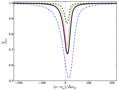
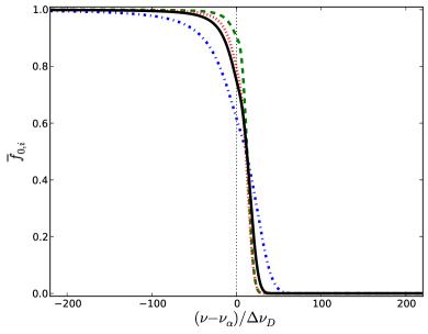
Figure 1.— Left: background radiation spectrum of the continuum photons around the Ly$\alpha$ frequency for the mean (unheated) temperature of $\overline{T}=10$ K and the mean density at $z=20$ (solid black line), normalized to the intensity of photons far away from the Ly$\alpha$ frequency. The spectrum shows an asymmetric absorption feature that results from combined contributions of scattering diffusivity and atomic recoil. Additional lines show how changing the conditions in the gas can modify the absorption feature: the green dashed line represents the solution for a five times higher mean temperature, the dash-dotted blue line is obtained for a five times higher mean density, and the red dotted line corresponds to the gas of an unaltered mean temperature and density, but with a significant velocity divergence. Right: same as on the left, but for the case of the injected photons.

To obtain the mean background solution $\overline{f}_{0\nu}$, we solve the unperturbed monopole equation (i.e., the equation for $l=0$ without any perturbative terms). For the continuum photons, the unperturbed equation is

$$H\nu_{\alpha}\frac{\partial\overline{f}_{0\nu}}{\partial\nu}+\frac{1}{\nu_{\alpha}^{2}}\frac{\partial}{\partial\nu}\left[\nu^{2}D_{\nu}\left(\frac{\partial\overline{f}_{0\nu}}{\partial\nu}+\frac{h}{k_{B}T}\overline{f}_{0\nu}\right)\right]=0$$

(23)

In solving this equation, we follow the procedure described in Chen & Miralda-Escudé (2004). The resulting spectrum (Figure 1, left panel), normalized to the intensity of photons on the blue side far away from the line center, shows an asymmetric absorption feature around the Ly$\alpha$ frequency. The shape of the feature is determined by the photon drift and diffusion in frequency caused by the scattering off of hydrogen atoms. This suppression in the radiation spectrum remains fixed once a steady state has been reached; it does not redshift away with the expansion of the universe, indicating energy transfer from the radiation field to the gas.

As shown in the left panel of Figure 1, the absorption feature is deeper for the gas of higher mean density (shown in blue dash-dotted line) because the scattering rate increases if there are more hydrogen atoms present. The feature is shallower for the gas of higher mean temperature (green dashed line) because in that case the energy transferred via recoils makes a smaller fraction of the average kinetic energy of the atoms. Similarly, the absorption feature is shallower for the case of non-zero atomic velocity divergence (red dotted line), which can be thought of as a bulk contribution to the kinetic energy of atoms in addition to their thermal motion. This explains why the feature changes in the same way as for an increase in temperature.

For the injected photons, the background equation has an extra term $\Psi=H\nu_{\alpha}\delta(\nu_{\alpha})$, resulting in a different spectral shape (Figure 1, right panel). If there were no scatterings, the photons would be injected at the Ly$\alpha$ frequency, and they would simply redshift to lower frequencies, creating a spectrum shaped as a step function. However, diffusion in frequency induced by scattering transfers some of the photons from the red side of the line to the blue side. This transfer is enhanced for the gas of higher mean density due to an increased scattering rate. Increasing the mean temperature of the gas and introducing bulk motions have the opposite effect, as in the case of the continuum photons. Injected photons cause cooling of the gas, as the upscattering of photons to the blue side extracts energy from it.

2.3. Perturbations

Perturbative terms in our equations have one of the following elements: perturbations to the photon distribution function $\delta f_{l\nu}$, non-zero velocity divergence $\delta_{\Theta}$, or perturbations to the diffusivity parameter $\delta_{D}$, which include density and temperature perturbations, $\delta_{n}$ and $\delta_{T}$, respectively. The full system of coupled differential equations including perturbative terms up to linear order is given in Appendix A. We numerically solve it to obtain spectra of perturbations for all multipole orders of interest. More details on the numerical implementation can be found in Appendix B. Figure 2 shows the lowest two orders ($l=0$ and $l=1$) in the expansion of the photon distribution function for different types of perturbations. Spectral features that arise for perturbations with wavenumbers in the range considered in this paper have characteristic widths that are on the order of several $\Delta\nu_{D}$ or greater, justifying the use of the Fokker-Planck approximation.

The resulting spectrum for $\delta f_{0}$ represents photons that are added (or subtracted, depending on whether $\delta f_{0}$ is positive or negative) to the mean solution $\overline{f}_{0}$ because of a small change in the gas temperature, density, or velocity. Since we are considering the photon phase space density in the frame of the gas, the dipole term $\delta f_{1}$ represents the photon flux into or out of a Lagrangian region of interest. It vanishes at the line center ($\nu\approx\nu_{\alpha}$) due to a very small mean free path of photons near the resonant frequency.

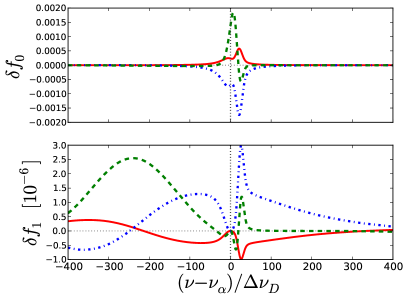
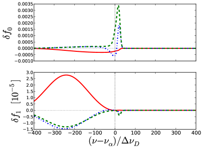
Figure 2.— Monopole and dipole terms of the perturbed radiation field for the continuum (left) and injected (right) photons, shown with the same normalization as in Figure 1. Different curves show the results obtained for different types of perturbations, all with the wavenumber $k=1$ cMpc^-1: green dashed curves correspond to $1\%$ temperature perturbations ($\delta_{T}=0.01$), blue dash-dotted lines represent $1\%$ perturbations in the density ($\delta_{n}=0.01$), and red solid lines show the results for introducing $1\%$ perturbation in the velocity divergence ($\delta_{\Theta}/H=0.01$) for the continuum photons and 10 times smaller perturbation in size and amplitude for the case of the injected photons.

3. Heating Rates

In the case of the continuum photons, the gas and the radiation field form a closed system whose energy is conserved. The rate at which the gas is heated thus equals the negative time change of the radiation energy:

$$\left[\frac{\partial U_{gas}}{\partial t}+\frac{\partial U_{rad}}{\partial t}\right]_{c}=0\ \mbox{,}$$ (24)

where $U$ is used to denote the energy density (in erg cm^-3) of the gas and radiation. The subscript $c$ indicates that this equation holds for the continuum photons. For the injected photons, however, there is an external source of energy that needs to be taken into account:

$$\left[\frac{\partial U_{gas}}{\partial t}+\frac{\partial U_{rad}}{\partial t}\right]_{i}=h\nu_{\alpha}\dot{N}_{i}\ \mbox{,}$$ (25)

where $\dot{N}_{i}$ is the generation rate of the injected photons.

The radiation energy density is given by

$$U_{rad}=\int n_{\nu}h\nu d\nu\ \ \mbox{.}$$ (26)

The number density of photons of frequency $\nu$ is $n_{\nu}$ (in units of cm^-3 Hz^-1). It is related to the specific intensity $J_{\nu}$ (intensity by the number of photons, not their energy, given in units of cm^-2 s^-1 Hz^-1 sr^-1) through the following relation

$$n_{\nu}=\frac{4\pi J_{\nu}}{c}=\frac{8\pi\nu^{2}f_{0\nu}}{c^{3}}\ \mbox{.}$$ (27)

Thus the photon energy density takes the form

$$U_{rad}=\frac{8\pi h}{c^{3}}\int\nu^{3}f_{0\nu}d\nu\ \ \mbox{,}$$ (28)

where the integral needs to be taken over a wide enough range around the Ly$\alpha$ frequency to include all significant spectral features. The gas heating rate per unit volume, given in units of erg cm^-3 s^-1, is the rate of change of the gas energy density $\Gamma\equiv\partial U_{gas}/\partial t$. For the sake of brevity, from now on we refer to $\Gamma$ simply as the heating rate. For the continuum photons, the heating rate is given by

$$\Gamma_{c}=-\frac{\partial U_{rad}}{\partial t}\bigg{|}_{c}=-\frac{8\pi h}{c^{3}}\int\nu^{3}\frac{\partial f_{0\nu}}{\partial t}\bigg{|}_{c}d\nu\ \mbox{.}$$ (29)

For the injected photons, there is an additional term

$$\Gamma_{i}=-\frac{8\pi h}{c^{3}}\int\nu^{3}\frac{\partial f_{0\nu}}{\partial t}\bigg{|}_{i}d\nu+h\nu_{\alpha}\dot{N}_{i}\mbox{.}$$ (30)

In the first term on the right side, we can make use of the expression for the time derivative of $f_{0\nu}$ given in Equation (21). Note that in the case of the injected photons, the source function $\Psi$ is non-zero. The photon injection rate in Equation (30) can be written as

$$\frac{\partial{N}_{i}}{\partial t} = \frac{\partial}{\partial t}\left(\int n_{i,\nu}d\nu\right)=\frac{\partial}{\partial t}\left(\int\frac{8\pi\nu^{2}}{c^{3}}f_{i}d\nu\right)$$ (31)

$$= \int\frac{8\pi\nu^{2}}{c^{3}}\frac{\partial f_{i}}{\partial t}d\nu=\int\frac{8\pi\nu^{2}}{c^{3}}\Psi d\nu$$

The two terms containing the source function cancel out - the injection of photons does not contribute to the gas heating rate. The heating of the gas is caused solely by the frequency diffusivity part of the collision term given by Equation (21).

The largest contribution to the gas heating rate comes from the part of the spectrum around the line center, thus it is convenient to separate the radiation energy density in the following way:

$$U=\frac{8\pi h}{c^{3}}\left[\nu_{\alpha}\int_{\nu_{1}}^{\nu_{2}}\nu^{2}f_{0\nu}d\nu+\int_{\nu_{1}}^{\nu_{2}}(\nu-\nu_{\alpha})\nu^{2}f_{0\nu}d\nu\right]\mbox{.}$$ (32)

The corresponding heating rate is

$$\Gamma=-\frac{8\pi h}{c^{3}}\biggl{[}\nu_{\alpha}\int_{\nu_{1}}^{\nu_{2}}\nu^{2}\frac{df_{0\nu}^{coll}}{dt}d\nu+\int_{\nu_{1}}^{\nu_{2}}(\nu-\nu_{\alpha})\nu^{2}\frac{df_{0\nu}^{coll}}{dt}d\nu\biggr{]}\mbox{.}$$ (33)

Using the expression given in Equation (21), the first term on the right side becomes

$$- \frac{8\pi h\nu_{\alpha}}{c^{3}}\int_{\nu_{1}}^{\nu_{2}}\frac{\partial}{\partial\nu}\left[\nu^{2}D_{\nu}\left(\frac{\partial f_{0\nu}}{\partial\nu}+\frac{h}{k_{B}T}f_{0\nu}\right)\right]d\nu$$ (34)

$$= -\frac{8\pi h\nu_{\alpha}}{c^{3}}\left[\nu^{2}D_{\nu}\left(\frac{\partial f_{0\nu}}{\partial\nu}+\frac{h}{k_{B}T}f_{0\nu}\right)\right]\bigg{|}_{\nu_{1}}^{\nu_{2}}\ \mbox{.}$$

The contribution of this term to the total heating rate is vanishingly small because $D_{\nu}$ approaches zero far from the line center. The remaining term is

$$\Gamma=-\frac{8\pi h}{c^{3}}\int_{\nu_{1}}^{\nu_{2}}(\nu-\nu_{\alpha})\frac{\partial}{\partial\nu}\left[\nu^{2}D_{\nu}\left(\frac{\partial f_{0\nu}}{\partial\nu}+\frac{h}{k_{B}T}f_{0\nu}\right)\right]d\nu$$

We can separate the heating rate into the contribution of the mean background radiation field and the contribution of the perturbations with

$$\Gamma=\overline{\Gamma}+e^{ikx_{3}}\delta\Gamma\ \mbox{,}$$ (35)

where $\overline{\Gamma}$ and $\delta\Gamma$ represent the background and perturbation heating, respectively. Making use of Equation (23) for the background heating rate, and an analogous expression for the case of perturbations, obtained from Equation (11), we get

$$\overline{\Gamma} = \frac{8\pi h}{c^{3}}\int_{\nu_{1}}^{\nu_{2}}(\nu-\nu_{\alpha})H\nu_{\alpha}^{3}\frac{\partial\overline{f}_{0\nu}}{\partial\nu}d\nu$$ (36)

$$= -\frac{8\pi h\nu_{\alpha}^{3}}{c^{3}}H(\nu-\nu_{\alpha})(\overline{f}_{\alpha}-\overline{f}_{0\nu})\bigg{|}_{\nu_{1}}^{\nu_{2}}$$

$$+\frac{8\pi h\nu_{\alpha}^{3}}{c^{3}}H\int_{\nu_{1}}^{\nu_{2}}(\overline{f}_{\alpha}-\overline{f}_{0\nu})d\nu\ \mbox{,}$$

$$\delta\Gamma = \frac{8\pi h}{c^{3}}\int_{\nu_{1}}^{\nu_{2}}\left(H\nu_{\alpha}^{3}\frac{\partial\delta f_{0\nu}}{\partial\nu}+\frac{\nu_{\alpha}^{3}\delta_{\Theta}}{3}\frac{\partial\overline{f}_{0\nu}}{\partial\nu}+\nu_{\alpha}^{2}kc\delta f_{1\nu}\right)$$ (37)

$$\times(\nu-\nu_{\alpha})d\nu$$

$$= \frac{8\pi h\nu_{\alpha}^{3}}{c^{3}}H\left[(\nu-\nu_{\alpha})\delta f_{\alpha}\bigg{|}_{\nu_{1}}^{\nu_{2}}-\int_{\nu_{1}}^{\nu_{2}}\delta f_{0\nu}d\nu\right]$$

$$-\frac{8\pi h\nu_{\alpha}^{3}\delta_{\Theta}}{3c^{3}}\left(\nu-\nu_{\alpha}\right)\left(\overline{f}_{\alpha}-\overline{f}_{0\nu}\right)\bigg{|}_{\nu_{1}}^{\nu_{2}}$$

$$+\frac{8\pi h\nu_{\alpha}^{3}\delta_{\Theta}}{3c^{3}}\int_{\nu_{1}}^{\nu_{2}}\left(\overline{f}_{\alpha}-\overline{f}_{0\nu}\right)d\nu$$

$$+\frac{8\pi h\nu_{\alpha}^{2}}{c^{3}}kc\int_{\nu_{1}}^{\nu_{2}}(\nu-\nu_{\alpha})\delta f_{1\nu}d\nu\ \mbox{,}$$

The above formulae are appropriate for frequencies around the line center. However, they might cause significant numerical errors in the wings of the line due to approximations made in deriving them. Hence, we use another expression to evaluate the heating rate in the wings:

$$\Gamma = -\frac{8\pi h}{c^{3}}\left[(\nu-\nu_{\alpha})\nu^{2}D_{\nu}\left(\frac{\partial f_{0\nu}}{\partial\nu}+\frac{h}{k_{B}T}f_{0\nu}\right)\bigg{|}_{\nu_{1}}^{\nu_{2}}\right]$$ (38)

$$+\frac{8\pi h}{c^{3}}\left[\int_{\nu_{1}}^{\nu_{2}}\nu^{2}D_{\nu}\left(\frac{\partial f_{0\nu}}{\partial\nu}+\frac{h}{k_{B}T}f_{0\nu}\right)d\nu\right]\ \mbox{.}$$

We report the calculated heating rates in terms of a dimensionless quantity, which we call the relative heating, that measures the energy transferred to the gas per Hubble time, relative to the thermal energy of the gas ($3\overline{n}k_{B}\overline{T}/2$):

$$\frac{\Gamma}{\frac{3}{2}\overline{n}k_{B}\overline{T}H(z)}=\frac{\overline{\Gamma}}{\frac{3}{2}\overline{n}k_{B}\overline{T}H(z)}+\frac{\delta\Gamma e^{ikx_{3}}}{\frac{3}{2}\overline{n}k_{B}\overline{T}H(z)}\ \ \mbox{,}$$ (39)

where $\overline{n}$ is the number density of all baryons, not just hydrogen atoms. Contributions of density, temperature, and velocity perturbations to the heating rate are incorporated into $\delta\Gamma$ and can be treated independently for each type of perturbation:

$$\delta\Gamma = \frac{\partial\Gamma}{\partial n}\delta_{n}+\frac{\partial\Gamma}{\partial T}\delta_{T}+\frac{\partial\Gamma}{\partial\Theta}\delta_{\Theta}\ \ \mbox{.}$$ (40)

Hence, the perturbative part of Equation (39) is given by

$$\frac{\delta\Gamma e^{ikx_{3}}}{\frac{3}{2}\overline{n}k_{B}\overline{T}H(z)}=\left[C_{n}\delta_{n}+C_{T}\delta_{T}+C_{\Theta}\frac{\delta_{\Theta}}{H}\right]\frac{\overline{J}_{\alpha}}{\tilde{J}_{0}}e^{ikx_{3}}\ \ \mbox{,}$$ (41)

where $\overline{J}_{\alpha}$ is the specific intensity of incoming photons and

$$\tilde{J}_{0}=\frac{n_{H}c}{4\pi\nu_{\alpha}}=\frac{2\nu_{\alpha}^{2}\tilde{f}_{0}}{c^{2}}$$ (42)

is the intensity corresponding to one photon per frequency octave per hydrogen atom in the universe (Chen & Miralda-Escudé, 2004). In terms of energy intensity, this corresponds to $\tilde{J}_{0}h\nu_{\alpha}\approx 2.5\times 10^{-20}$ erg cm^-2 s^-1 sr^-1 Hz^-1 at $z=20$. In the model of Ciardi & Madau (2003), the intensity of Ly$\alpha$ background at $z\sim 20$ is on the order of $10^{-20}$ erg cm^-2 s^-1 sr^-1 Hz^-1, making $\overline{J}_{\alpha}/\tilde{J}_{0}$ a factor of order unity. In general, one expects it to be a rapidly increasing function of redshift. Since it takes $\geq 1$ H-ionizing ($\nu>\frac{4}{3}\nu_{\alpha}$) photons per atom to ionize the universe, and since the non-ionizing photons that redshift into Lyman series lines do not suffer from absorption in the emitting galaxies, we expect that $\overline{J}_{\alpha}/\tilde{J}_{0}$ should reach unity at an early stage of reionization (Chen & Miralda-Escudé, 2004).

We have defined dimensionless heating coefficients $C$ for all three types of perturbations by

$$C_{n} = \frac{2\tilde{f}_{0}}{3\overline{n}k_{B}\overline{T}H}\frac{\partial\Gamma}{\partial n}\ \mbox{,}$$ (43)

$$C_{T} = \frac{2\tilde{f}_{0}}{3\overline{n}k_{B}\overline{T}H}\frac{\partial\Gamma}{\partial T}\ \mbox{,~{}and}$$ (44)

$$C_{\Theta} = \frac{2\tilde{f}_{0}}{3\overline{n}k_{B}\overline{T}}\frac{\partial\Gamma}{\partial\Theta}\ \mbox{;}$$ (45)

these represent the heat input per Hubble time in units of the thermal energy of the gas, if $\overline{J}_{\alpha}/\tilde{J}_{0}=1$.

4. Results and Discussion

We perform calculations described in the previous sections for neutral hydrogen gas ($x_{HI}=1$) at the redshift of $z=20$. The mean baryon number density is easily obtained from the current baryon density of the universe $\overline{n}_{0}=2.5\times 10^{-7}$ cm^-3 (WMAP-9 result, Bennett et al. 2012) as $\overline{n}(z)=\overline{n}_{0}(1+z)^{3}$. Finally, to get the number density of hydrogen atoms we take into account that over $90\%$ (by number) of the baryonic content is in the form of hydrogen atoms. For the mean temperature of the gas we take the value $\overline{T}=10$ K (see Figure 1 in Pritchard & Furlanetto 2006).

4.1. Heating from Unperturbed Radiation

The calculated contribution to the relative heating coming from the mean (unperturbed) background photons can be expressed as

$$\frac{\overline{\Gamma}_{c}}{\frac{3}{2}\overline{n}k_{B}\overline{T}H}=0.13\frac{\overline{J}_{\alpha,c}}{{J}_{0}}\$$ (46)

for the continuum photons, and as

$$\frac{\overline{\Gamma}_{i}}{\frac{3}{2}\overline{n}k_{B}\overline{T}H}=-0.07\frac{\overline{J}_{\alpha,i}}{{J}_{0}}$$ (47)

for the injected photons. The relative heating caused by the scattering of the injected photons is negative, indicating that the gas is cooled down by this interaction. At this temperature and density, heating of the gas caused by the scattering of the continuum photons prevails over cooling by the injected photons, not only because the effect itself is slightly stronger, but also because the flux of the injected photons is smaller than the flux of the continuum photons; the ratio of the injected and continuum photons is around 10$\%$-20$\%$ (Pritchard & Furlanetto, 2006; Chuzhoy & Shapiro, 2007).

4.2. Heating from Perturbations

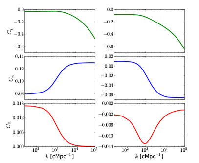
Figure 3.— Heating coefficients, defined by expressions (43) - (45), for the continuum (left) and injected photons (right) show contributions of temperature, density, and velocity perturbations (from top to bottom) to the total heating rate as functions of the perturbation wavenumber $k$, given in comoving units.

A new result of this study is the additional contribution to the relative heating caused by inhomogeneities in the gas. The differential relative heating due to perturbations is given by Equation (41). The values of all three heating coefficients $C$ for perturbations of different wavenumbers $k$ are shown in Figure 3.

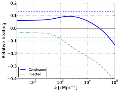
Figure 4.— Solid and dotted lines show the joint contribution of the temperature and density perturbations to the relative heating for the continuum and injected photons, respectively, as a function of perturbation wavenumber (comoving). These values need to be multiplied by the amplitude of the density perturbations to give the perturbative heating that can then be compared to the unperturbed effect, shown in dashed and dash-dotted lines. On very small scales, the perturbative heating from the continuum photons changes sign relative to the mean effect, causing damping of small scale perturbations. The same does not occur for the injected photons - they cause negative heating (i.e., cooling) of gas on all scales. Their contribution relative to the continuum photons is diminished by the fact that their intensity is lower, making only $\sim 10\%-20\%$ of the intensity of the continuum photons.

On large scales, corresponding to small values of the wavenumber $k$, having a positive perturbation in the temperature or density is similar to having a region with no perturbations, but with an increased mean value. As shown in Figure 1 and discussed in Section 2.1, an increase in $\overline{T}$ causes the absorption feature in the spectrum of $\overline{f}_{0}$ to be shallower, whereas an increase in $\overline{n}$ makes the feature deeper. The heating is proportional to the integral of the difference between the spectrum without any scattering (which is just a flat spectrum for the case of the continuum photons) and the real spectrum, hence it is proportional to the area of the absorption feature. Therefore, the heating will be smaller in the case of higher $\overline{T}$, which is why $C_{T}$ has negative values on large scales. On the other hand, $C_{n}$ is positive, since an increase in $\overline{n}$ causes a larger heating. The absolute values of heating coefficients increase for larger values of $k$, indicating that these effects are enhanced on smaller scales in the case of the continuum photons.

To estimate the contribution of perturbations to the total heating of the gas, we need to know the relative strengths of different kinds of perturbations, in addition to the values of the heating coefficients. Naoz & Barkana (2005) calculated the ratio of temperature and density perturbations as a function of wavenumber $k$ at several redshifts, including $z=20$, the epoch that we consider in this work. The ratio of $\delta_{T}$ and $\delta_{n}$ at $z=20$ is almost constant for small-scale perturbations, $\delta_{T}/\delta_{n}\approx 0.55$. We make use of this result to show (Figure 4) the joint contribution of the density and temperature perturbations ($C_{n}+0.55C_{T}$) relative to the heating caused by the unperturbed background photons. We ignore perturbations in the velocity because the magnitude of $C_{\Theta}$ is much smaller than that of $C_{T}$ or $C_{n}$ for most wavenumbers.

On large scales (i.e., small values of $k$), the heating caused by perturbations has the same sign as the mean effect: positive for the continuum photons and negative for the injected photons, which indicates a small increase in the gas heating by the continuum photons in regions of higher density and temperature due to the increased scattering rate. Cooling by the injected photons in those regions will also increase. These additional contributions to the heating are very small. The values shown in Figure 4, which are already a factor of $\sim 2$ smaller than the mean effect, need to be multiplied by the amplitude of density perturbations to give the actual relative heating. Since our formalism is based on the linear perturbation theory, it is applicable to perturbations of the order of a few percent or smaller. Hence, the additional heating at large scales can only make a few percent of the mean (unperturbed) Ly$\alpha$ heating.

An interesting feature appears for perturbations on very small scales ($k\sim 2\times 10^{4}$ cMpc^-1). For the case of the continuum photons, values of the relative heating, shown in Figure 4, turn from positive to negative. On length scales below that threshold, perturbations act in the opposite direction from the unperturbed effect; they reduce the heating of the gas in positively perturbed regions (i.e., regions of higher density and temperature than the mean). The opposite happens for cooler and underdense regions. The effect of the injected photons remains unchanged. Hence, perturbations on scales smaller than that corresponding to $k\sim 2\times 10^{4}$ cMpc^-1 will be damped due to the effect of thermal conduction by Ly$\alpha$ photons. This length scale, however, is roughly two orders of magnitude smaller than the Jeans scale.

For gas of higher mean temperature, e.g., with $\overline{T}=20$ K, the result stays qualitatively the same, only the values of the relative heating, both the mean effect and the contribution of perturbations, are reduced.

5. Conclusions

The resonant scattering of Ly$\alpha$ photons produced by early generations of luminous objects can cause moderate heating of high-redshift IGM. Ly$\alpha$ photons and hydrogen atoms exchange energy during scattering due to atomic recoil. Details of radiative transfer are further complicated by the frequency diffusion of photons caused by scattering and the drift to lower frequencies due to Hubble expansion. In the optically thick limit, the gas and the radiation field approach statistical equilibrium, which greatly reduces the energy exchange. Taking into account all of these effects, an asymmetric absorption feature is created in the radiation spectrum around the Ly$\alpha$ frequency in the case of the continuum photons that redshift directly into Ly$\alpha$ from the blue side of the line. Photons that redshift into higher resonances and then cascade into Ly$\alpha$ are called the injected photons. Their spectrum has a shape of a modified step function around the Ly$\alpha$ frequency. Scattering of the continuum photons causes heating of the IGM proportional to the area of the absorption feature. This heating is higher for gas of lower mean temperature and higher density. The injected photons, on the other hand, cause cooling of the gas because they preferentially scatter off atoms moving in the opposite direction.

In this paper, we study the effect of Ly$\alpha$ scattering on high-redshift ($z=20$) IGM with linear perturbations in density, temperature, and velocity divergence. We are primarily interested in small-scale perturbations that can be affected by thermal conduction via Ly$\alpha$ photons. For perturbations with scales smaller than the Ly$\alpha$ diffusion length-scale, photons can diffuse into regions where they are further away from being in a statistical equilibrium with the gas, causing enhancement in the energy exchange. To find the exact scale at which this occurs, we solve radiative transfer equations numerically, using the Fokker-Planck approximation.

We find that the scale at which this effect becomes relevant is very small, corresponding to a comoving wavenumber of $k\sim 2\times 10^{4}$ Mpc^-1, which is a factor of $\sim 100$ smaller than the Jeans scale. On larger scales, where structures in the IGM are expected to be present, the heating perturbations add a correction to the mean effect that is on the order of the amplitude of the density or temperature perturbation in the gas. Since our formalism is based on the linear perturbation theory, this makes only a few percent difference to the gas heating in typical cases.

Appendix A System of equations

Equations for different multipoles of the perturbed radiation field are given by:

$$H\nu\frac{\partial\delta f_{0\nu}}{\partial\nu}+\frac{1}{3}\nu\delta_{\Theta}\frac{\partial\overline{f}_{0\nu}}{\partial\nu} + kc\delta f_{1\nu}+\frac{\partial\overline{D}_{\nu}}{\partial\nu}\left(\frac{\partial\delta f_{0\nu}}{\partial\nu}+\frac{h}{k_{B}T}\delta f_{0\nu}\right)+\frac{\partial\overline{D}_{\nu}}{\partial\nu}\delta_{D}\left(\frac{\partial\overline{f}_{0\nu}}{\partial\nu}+\frac{h}{k_{B}T}\overline{f}_{0\nu}\right)+$$ (A1)

$$+ \overline{D}_{\nu}\left(\frac{\partial^{2}\delta f_{0\nu}}{\partial\nu^{2}}+\frac{h}{k_{B}T}\frac{\partial\delta f_{0\nu}}{\partial\nu}\right)+\overline{D}_{\nu}\delta_{D}\left(\frac{\partial^{2}\overline{f}_{0\nu}}{\partial\nu^{2}}+\frac{h}{k_{B}T}\frac{\partial\overline{f}_{0\nu}}{\partial\nu}\right)=0\ \mbox{,}\ \ \ \mbox{$(l=0)$}$$

$$H\nu\frac{\partial\delta f_{1\nu}}{\partial\nu}-\frac{kc}{3}\left(\delta f_{0\nu}-2\delta f_{2\nu}\right)-n_{H}c\sigma(\nu,T)\delta f_{1\nu}=0\ \mbox{,}\ \ \ \mbox{$(l=1)$}$$ (A2)

$$H\nu\frac{\partial\delta f_{2\nu}}{\partial\nu}-\frac{2}{15}\nu\delta_{\Theta}\frac{\partial\overline{f_{0\nu}}}{\partial\nu}-\frac{kc}{5}\left(2\delta f_{1\nu}-3\delta f_{3\nu}\right)-n_{H}c\sigma(\nu,T)\delta f_{2\nu}=0\ \mbox{,}\ \ \ \mbox{$(l=2)$}$$ (A3)

$$\cdots$$

$$H\nu\frac{\partial\delta f_{l_{max}\nu}}{\partial\nu} - \frac{kc}{2l_{max}+1}\left(l_{max}\delta f_{\left(l_{max}-1\right)\nu}-(l_{max}+1)\delta f_{\left(l_{max}+1\right)\nu}\right)-n_{H}c\sigma(\nu,T)\delta f_{l_{max}\nu}=0\ \mbox{,}\ \ \ \mbox{$(l=l_{max})$}$$ (A4)

where $k$ is the physical wavenumber, not comoving. In the first equation, $\overline{D}_{\nu}$ is used to denote the mean value of the diffusivity parameter. The full expression for this quantity, including perturbations, can be written as $D_{\nu}=\overline{D}_{\nu}(1+\delta_{D})=\overline{D}_{\nu}(1+\delta_{n}+\delta_{T})$.

Appendix B Numerical calculations

To solve the above described system of equations, we truncate the series at $l_{max}=8$ by setting $\delta f_{9\nu}=0$. The choice of the largest considered multipole could of course be different. In our analysis, we only use the solutions for the monopole and dipole terms, but we want to keep as many higher orders as possible to avoid introducing significant errors into the lowest multipoles by making an artificial truncation of the series too close to them. On the other hand, tracking too many multipole orders becomes computationally challenging. We find that keeping nine multipoles is optimal: the computation can be done in a reasonable amount of time and increasing $l_{max}$ by one changes the resulting heating rate by $2\%$ at most (in most cases much less than that).

Once we have a finite set of differential equations, we create an equidistant frequency grid containing a large number ($7\times 10^{5}$) of frequencies centered at $\nu_{\alpha}$. The frequency range covered in our grid spans $3.3\times 10^{12}$ Hz (corresponding to $\sim 1000\ \Delta\nu_{D}$) on each side of the Ly$\alpha$ frequency. These numbers could have been chosen differently without significantly affecting the final result. For example, decreasing the frequency range by $10\%$ changes the computed heating rate by no more than $1\%-2\%$. We can change the size of the frequency grid to test the convergence of our method. Increasing the number of frequencies in the grid spanning the same frequency range to $8\times 10^{5}$ changes the result by $\sim 2\%$ or less.

In order to avoid numerical errors that can occur near the boundaries of the grid, in our calculations we do not take into account outer $3\times 10^{4}$ frequencies at both ends of the grid. As mentioned in Section 3, to calculate the heating rate we use Equations (36) and (37) in the central part of the grid and Equation (38) in the outer parts. The exact number of frequencies included in these outer parts, the so-called wings, does not significantly affect the result, as long as the central spectral features, contained within $\sim 100\Delta\nu_{D}$ of the Ly$\alpha$ line center, are not included. The difference between having $\sim 20\%$ of frequencies in the wings and having $40\%$ is less than $4\%$.

For the described grid of $7\times 10^{5}$ frequencies and with 9 multipoles, our system of equations forms a matrix of dimension $(9\times 7\times 10^{5})\times(9\times 7\times 10^{5})$. Manipulating such a large matrix can be challenging. Fortunately, most of the elements of this matrix are zero, hence we make use of SciPy sparse matrix package (scipy.sparse) to construct the matrix and solve the sparse linear system.

To approximate differentiation in the equations, we first used the central difference method

$$f^{\prime}(\nu)=\frac{f(\nu+\Delta\nu)-f(\nu-\Delta\nu)}{2\Delta\nu}+\mathcal{O}(\Delta\nu^{2})\mbox{,}$$ (B1)

where $\Delta\nu$ is the grid step. However, due to numerical oscillations that occurred near the end of the frequency grid, we introduced dissipation in the form of the forward difference contribution

$$f^{\prime}(\nu)=\frac{f(\nu+\Delta\nu)-f(\nu)}{\Delta\nu}+\mathcal{O}(\Delta\nu)\mbox{.}$$ (B2)

Hence, the derivatives are given by a linear combination of the central and forward difference terms

$$f^{\prime}(\nu)=\epsilon\frac{f(\nu+\Delta\nu)-f(\nu)}{\Delta\nu}+\left(1-\epsilon\right)\frac{f(\nu+\Delta\nu)-f(\nu-\Delta\nu)}{2\Delta\nu}\ \mbox{.}$$ (B3)

Parameter $\epsilon$ describes the contribution of the forward difference method, and it changes linearly from zero at the center to unity at the ends of the frequency grid.

References

- Bennett et al. (2012) Bennett, C. L., Larson, D., Weiland, J. L., et al. 2013, ApJS, 208, 20
- Bowman & Rogers (2010) Bowman, J. & Rogers, A. 2010, Nature, 468, 796
- Chen & Miralda-Escudé (2004) Chen, X. & Miralda-Escudé, J. 2004, ApJ, 602, 1
- Chuzhoy & Shapiro (2007) Chuzhoy, L. & Shapiro, P. R. 2007, ApJ, 655, 843
- Ciardi & Madau (2003) Ciardi, B. & Madau, P. 2003, ApJ, 569, 1
- Ciardi & Salvaterra (2007) Ciardi, B. & Salvaterra, R. 2007, MNRAS, 381, 1137
- Dillon et al. (2013) Dillon, J., Liu, A., Williams, C. L., et al. 2013, arXiv:1304.4229
- Field (1958) Field, G. B. 1958, PIRE, 46, 240
- Furlanetto, Oh & Briggs (2006) Furlanetto, S. R., Oh, S. P. & Briggs, F. H. 2006, PhR, 433, 181
- Furlanetto & Pritchard (2006) Furlanetto, S. R. & Pritchard, J. R. 2006, MNRAS, 372, 1093
- Higgins & Meiksin (2009) Higgins, J. & Meiksin, A. 2009, MNRAS, 393, 949
- Higgins & Meiksin (2012) Higgins, J. & Meiksin, A. 2012, MNRAS, 426, 2380
- Hirata (2006) Hirata, C. M. 2006, MNRAS, 367, 259
- Hu et al. (1995) Hu, W., Scott, D., Sugiyama, N. & White, M. 1995, PhRvD, 52, 5498
- Lonsdale et al. (2009) Lonsdale, C., Cappallo, R. J., Morales, M. F., et al. 2009, IEEEP, 97, 1497
- Ma & Bertschinger (1995) Ma, C. & Bertschinger, E. 1995, ApJ, 455, 7
- Madau, Meiksin & Rees (1997) Madau, P., Meiksin, A. & Rees, M. J. 1997, ApJ, 475, 429
- Meiksin (2006) Meiksin, A. 2006, MNRAS, 370, 2025
- Morales & Wyithe (2010) Morales, M. F. & Wyithe, J. S. B. 2010, ARA&A, 48, 127
- Naoz & Barkana (2005) Naoz, S. & Barkana, R. 2005, MNRAS, 362, 1047
- Paciga et al. (2013) Paciga, G., Albert, J. G., Bandura, K., et al. 2013, MNRAS, 443, 639
- Parsons et al. (2013) Parsons, A., Liu, A., Aguirre, J. E., et al. 2013, arXiv:1304.4991
- Parsons et al. (2012) Parsons, A., Pober, J., McQuinn, M., Jacobs, D., & Aguirre, J. 2012, ApJ, 753, 81
- Planck Collaboration (2013) Planck Collaboration 2013, arXiv:1303.5076
- Pritchard & Furlanetto (2006) Pritchard, J. R. & Furlanetto, S. R. 2006, MNRAS, 367, 1057
- Pritchard & Loeb (2012) Pritchard, J. R. & Loeb, A. 2012, RPPh, 75, 6901
- Rawlings & Schilizzi (2011) Rawlings, S. & Schilizzi, R. 2010, in Proc. Joint Science with the E-ELT and SKA, ed I. Hook et al. (Voutes Heraklion: Crete Univ. Press), (arXiv:1105.5953)
- Rybicki (2006) Rybicki, G. B. 2006, ApJ, 647, 709
- Rybicki & Dell’Antonio (1994) Rybicki, G. B. & Dell’Antonio, I. P. 1994, ApJ, 427, 603
- van Haarlem et al. (2013) van Haarlem, M. Wise, M. W., Gunst, A. W., et al. A&A, 556, A2
- Wouthuysen (1952) Wouthuysen, S. A. 1952, AJ, 57, 31