Numerical studies of space filling designs: optimization of Latin Hypercube Samples and subprojection properties

Abstract

Quantitative assessment of the uncertainties tainting the results of computer simulations is nowadays a major topic of interest in both industrial and scientific communities. One of the key issues in such studies is to get information about the output when the numerical simulations are expensive to run. This paper considers the problem of exploring the whole space of variations of the computer model input variables in the context of a large dimensional exploration space. Various properties of space filling designs are justified: interpoint-distance, discrepancy, minimum spanning tree criteria. A specific class of design, the optimized Latin Hypercube Sample, is considered. Several optimization algorithms, coming from the literature, are studied in terms of convergence speed, robustness to subprojection and space filling properties of the resulting design. Some recommendations for building such designs are given. Finally, another contribution of this paper is the deep analysis of the space filling properties of the design 2D-subprojections.

Keywords: discrepancy, optimal design, Latin Hypercube Sampling, computer experiment.

1 Introduction

Many computer codes, for instance simulating physical phenomena and industrial systems, are too time expensive to be directly used to perform uncertainty, sensitivity, optimization or robustness analyses (de Rocquigny et al.,, 2008). A widely accepted method to circumvent this problem consists in replacing such computer models by cpu time inexpensive mathematical functions, called metamodels (Kleijnen and Sargent,, 2000), built from a limited number of simulation outputs. Some commonly used metamodels are: polynomials, splines, generalized linear models, or learning statistical models like neural networks, regression trees, support vector machines and Gaussian process models (Fang et al.,, 2006). In particular, the efficiency of Gaussian process modelling has been proved for instance by Sacks et al., (1989); Santner et al., (2003); Marrel et al., (2008). It extends the kriging principles of geostatistics to computer experiments by considering that the code responses are correlated according to the relative locations of the corresponding input variables.

A necessary condition to successful metamodelling is to explore the whole space $\mathcal{X}\subset{\mathbb{R}}^{d}$ of the input variables ${\mathbf{X}}\in\mathcal{X}$ (called the inputs) in order to capture the non linear behaviour of some output variables ${\mathbf{Y}}=G({\mathbf{X}})\in{\mathbb{R}}^{q}$ (where $G$ refers to the computer code). This step, often called the Design of Computer Experiments (DoCE), is the subject of this paper. In many industrial applications, we are faced with the harsh problem of the high dimensionality of the space $\mathcal{X}$ to explore (several tens of inputs). For this purpose, Sample Random Sampling (SRS), that is standard Monte-Carlo, can be used. An important advantage of SRS is that the linear variability of estimates of quantities such as mean output behaviour is independent of $d$, the dimension of the input space.

However, some authors (Simpson et al.,, 2001; Fang et al.,, 2006) have shown that the Space Filling Designs (SFD) are well suited to this initial exploration objective. A SFD aims at obtaining the best coverage of the space of the inputs, while SRS does not ensure this task. Moreover, the SFD approach appears natural in first exploratory phase, when very few pieces of information are available about the numerical model, or if the design is expected to serve different objectives (for example, providing a metamodel usable for several uncertainty quantifications relying on different hypothesis about the uncertainty on the inputs). However, the class of SFD is diverse including the well-known Latin Hypercubes Samples (LHS) , Orthogonal Arrays (OA), point process designs (Franco et al.,, 2008), minimax and maximin designs each based on a distance criterion (Johnson et al.,, 1990; Koehler and Owen,, 1996), maximum entropy designs (Schwery and Wynn,, 1987). Another kind of SFD is the one of Uniform Designs (UD) whose many interests for computer experiments have been already discussed (Fang and Lin,, 2003). They are based upon some measures of uniformity called discrepancies (Niederreiter,, 1987). Here, our purpose is to shed new light on the practical issue of building a SFD.

In the following, $\mathcal{X}$ is assumed to be ${[0;1]}^{d}$, up to a bijection. Such a bijection is never unique and different ones generally lead to non equivalent ways of filling the space of the inputs. In practice, during an exploratory phase, only pragmatic answers can be given to the question of the choice of the bijection: maximum and minimum bounds are generally given to each scalar input so that $\mathcal{X}$ is an hypercube which can be mapped over ${[0;1]}^{d}$ through a linear transformation. It can be noticed that, if there is a sufficient reason to do so, it is always possible to apply simple changes of input variables if it seems relevant (e.g. considering the input $z=\exp(x)\in[\exp(a),\exp(b)]$ instead of $x\in[a,b]$).

In what follows, we focus on the “homogeneous” filling of ${[0;1]}^{d}$ and the main question addressed is how to build or to select a DoCE of a given (and small) size $N$ ($N\sim 100$, typically) within ${[0;1]}^{d}$ (where $d>10$, typically). We keep also in mind the well-known and empirical relation $N\sim 10d$ (Loeppky et al.,, 2009; Marrel et al.,, 2009) which gives the approximative minimum number of computations needed to get an accurate metamodel.

A first consideration is to obtain the best global coverage rate of ${[0;1]}^{d}$. In the following, quality of filling is improved by optimizing discrepancies or point-distance criteria and assessed by robust geometric criteria based on the Minimum Spanning Tree (MST) (Dussert et al.,, 1986). When building SFD upon a particular criterion, a natural prerequisite is coordinate rotation invariance, that is invariance of the value of the criterion under exchanges of coordinates. Criteria applied hereafter are coordinate rotation invariant. An important prescription is to properly cover the variation domain of each scalar input. Indeed, it often happens that, among a large number of inputs, only a small one is active, that is significantly impacts the outputs (sparsity principle). Then, in order to avoid useless computations (different values for inactive inputs but same values for active ones), we have to ensure that all the values for each input are different, which can be achieve by using LHS. A last important property of a SFD is its robustness to projection over subspaces. This property is particularly studied in this paper and the corresponding results can be regarded as the main contributions. Literature about the application of the physical experimental design theory shows that, in most of the practical cases, effects of small degree (involving few factors, that is few inputs) dominates effects of greater degree. Therefore, it seems judicious to favour a SFD whose subprojections offer some good coverages of the low-dimensional subspaces. A first view, which is adopted here, is to explore two-dimensional (2D) subprojections.

Section 2 describes two industrial examples in order to motivate our concerns about SFD. Section 3 gives a review about coverage criteria and natures of SFD studied in the next section. The preceding considerations lead us to focus our attention on optimized LHS for which various optimization algorithms have been previously proposed (main works are Morris and Mitchell, (1995) and Jin et al., (2005)). We adopt a numerical approach to compare the performance of different LHS, in terms of their interpoint-distance and $L^{2}$-discrepancies. Section 4 focuses on their 2D subprojection properties and numerical tests support some recommendations. Section 5 synthesizes the work.

2 Motivating examples

2.1 Nuclear safety simulation studies

Assessing the performance of nuclear power plants during accidental transient conditions has been the main purpose of thermal-hydraulic safety research for decades. Sophisticated computer codes have been developed and are now widely used. They can calculate time trends of any variable of interest during any transient in Light Water Reactors (LWR). However, the reliability of the predictions cannot be evaluated directly due to the lack of suitable measurements in plants. The capabilities of the codes can consequently only be assessed by comparison of calculations with experimental data recorded in small-scale facilities. Due to this difficulty, but also the “best-estimate” feature of the codes quoted above, uncertainty quantification should be performed when using them. In addition to uncertainty quantification, sensitivity analysis is often carried out in order to identify the main contributors to uncertainty.

Those thermal-hydraulic codes enable, for example, to simulate a large-break loss of primary coolant accident (see Figure 1). This scenario is part of the Benchmark for Uncertainty Analysis in Best-Estimate Modelling for Design, Operation and Safety Analysis of Light Water Reactors (de Crécy et al.,, 2008) proposed by the Nuclear Energy Agency of the Organisation for Economic Co-operation and Development (OCDE/NEA). It has been implemented on the French computer code CATHARE2 developed at the Commissariat à l’Energie Atomique (CEA). Figure 2 illustrates $100$ Monte Carlo simulations (by randomly varying the inputs of the accidental scenario), given by CATHARE2, of the cladding temperature in function of time, whose first peak is the main output of interest in safety studies.

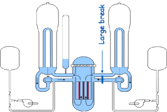
Figure 1: Illustration of a large-break loss of primary coolant accident on a nuclear Pressurized Water Reactor (a particular but common type of LWR).

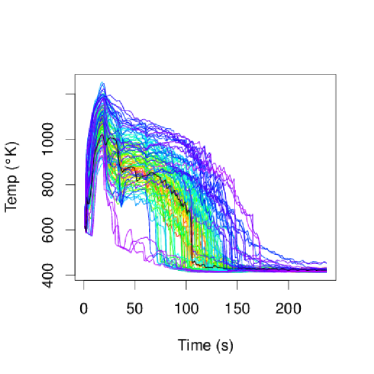
Figure 2: $100$ output curves of the cladding temperature in function of time from CATHARE2.

Severe difficulties arise when carrying out a sensitivity analysis or an uncertainty quantification involving CATHARE2:

• Physical models involve complex phenomena (non linear and subject to threshold effects), with strong interactions between inputs. A first objective is to detect these interactions. Another one is to fully explore combinations of the input to obtain a good idea of the possible transient curves (Auder et al.,, 2012).

• Computer codes are cpu time expensive: no more than several hundreds of simulations can be performed.

• Numerical models take as inputs a large number of uncertain variables ($d=50$, typically): physical laws essentially, but also initial conditions, material properties and geometrical parameters. Truncated normal or log-normal distributions are given to them. Such a number of inputs is extremely large for the metamodelling problem.

• The first peak of the cladding temperature can be related to rare events: problems turn to the estimation of a quantile (Cannamela et al.,, 2008) or the probability that the output exceeds a threshold (Marrel and Marquès,, 2012).

All of these four difficulties underline the fact that great care is required to define an effective DoCE over the CATHARE2 input space. The high dimension of the input space remains a challenge for building a SFD with good subprojection properties.

2.2 Prey-predator simulation chain

In ecological effect assessments, risks imputable to chemicals are usually estimated by extrapolation of single-species toxicity tests. With increasing awareness of the importance of indirect effects and keeping in mind limitations of experimental tools, a number of ecological food-web models have been developed. Such models are based on a large set of bioenergetic equations describing the fundamental growth of each population, taking into account grazing and predator-prey interactions, as well as influence of abiotic factors like temperature, light and nutrients. They can be used for several purposes, for instance:

• to test various contamination scenarios or recovery capacity of contaminated ecosystem,

• to quantify the important sources of uncertainty and knowledge gaps for which additional data are needed, and to identify the most influential parameters of population-level impacts,

• to optimize the design of field or mesocosm tests by identifying the appropriate type, scale, frequency and duration of monitoring.

Following this rationale, an aquatic ecosystem model, MELODY, was built so as to simulate the functioning of aquatic mesocosms as well as the impact of toxic substances on the dynamics of their populations. A main feature of this kind of ecological model is, however, the great number of parameters involved in the modelling: MELODY has a total of 13 compartments and 219 parameters; see Figure 3. These are generally highly uncertain because of both natural variability and lack of knowledge. Thus, sensitivity analyses appears an essential step to identify non-influential parameters (Ciric et al.,, 2012). These can then be fixed at a nominal value without significantly impacting the output. Consequently, the calibration of the model becomes less complex (Saltelli et al.,, 2006).

Figure 3: Representation of the module chain of the aquatic ecosystem model MELODY.

By a preliminary sensitivity analysis of the periphyton-grazers submodel (representative of processes involved in dynamics of primary producers and primary consumers and involving $20$ input parameters), Iooss et al., (2012) concludes that significant interactions of large degrees (more than three) exist in this model. Therefore, a DoCE has to possess excellent subprojection properties to capture the interaction effects.

3 Space filling criteria and designs

Building a DoCE consists in generating a matrix $\mathbf{X}^{N}_{d}=(x_{j}^{(i)})_{i=1..N,j=1..d}$, where $N$ is the number of experiments and $d$ the number of scalar inputs. The $i^{th}$ line $x^{(i)}$ of this matrix will correspond to the inputs of the $i^{th}$ code execution. Let us recall that, here, the purpose is to design $N$ experiments $x^{(i)}$ to fill as “homogeneously” as possible the set $\mathcal{X}={[0;1]}^{d}$; even if, in an exploratory phase, a joint probability distribution is not explicitly given to the inputs, one can consider that this distribution is uniform over $\mathcal{X}$. In fact, some space-filling criteria discussed hereafter do not formally refer to the uniform distribution (but geometric considerations), yet they share with it the property of not favouring any particular area of $\mathcal{X}$.

The most common sampling method is indisputably the classical Monte Carlo (Simple Random Sampling, SRS), mainly because of its simplicity and generality (Gentle,, 2003), but also because of the difficulty to sample in a more efficient manner when $d$ is large as well. In our context, it would consist in randomly, uniformly and independently sampling $d\times N$ draws in $[0;1]$. SRS is largely used to propagate uncertainties through computer codes (de Rocquigny et al.,, 2008) because it has the attractive property of giving a convergence rate for estimates of quantities like expectations that is $O(N^{-1/2})$. This convergence rate is independent of $d$, the dimension of the input space.

Yet, SRS is known to possess poor space filling properties: SRS leaves wide unexplored regions and may draw very close points. Quasi-Monte Carlo sequences (Lemieux,, 2009) furnish good space filling properties, giving a better convergence rate ($O((\log N)^{d}/N)$) for estimates of expectations. If, in practice, improvement over SRS is not attained when $d$ is large, dimensionality can be controlled by methods of dimension reduction such as stratified sampling (Cheng and Davenport,, 1989) and sensitivity analysis (Varet et al.,, 2012).

The next sections are mainly dedicated to (optimized) LHS, owing to their property of parsimony mentioned in the introduction, and do not refer to other interesting classes of SFD, neither maximum entropy designs nor point process designs in particular. The former is based on a criterion (Shannon entropy) to maximize which could be used to optimize LHS. The resulting SFD is similar to point-distance optimized LHS (section 3.2.2), as shown by theoretical works (Pronzato and Müller,, 2012) and confirmed by our own experiments. The latter way of sampling seems hardly compatible with LHS and suffers from the lack of efficient rules to set its parameters (Franco,, 2008).

In this section, criteria used hereafter to make diagnosis of DoCE or to optimize LHS are defined. Computing optimized LHS requires an efficient, in fact specialized, optimization algorithm. Since the literature provides numerous ones, a brief overview of a selection of such algorithms is proposed. The section ends with our feedback on their behaviours, with an emphasis on maximin DoCE.

3.1 Latin Hypercube Sampling

Latin Hypercube Sampling, which is an extension of stratified sampling, aims at ensuring that each of the scalar input has the whole of its range well scanned, according to a probability distribution (McKay et al.,, 1979; Fang et al.,, 2006). Below, LHS is introduced in our particular context, that is considering a uniform distribution over ${[0;1]}^{d}$, for the sake of clarity.

Let the range $[0;1]$ of each input variable $X_{j}$, $j=1\ldots d$, be partitioned into $N$ equally probable intervals $\mathcal{I}_{k}=(\frac{k-1}{N}~{};\frac{k}{N})$, $k=1\ldots N$. The definition of a LHS requires $d$ permutations $\pi_{j}$ of $\{1,\ldots,N\}$, which are randomly chosen (uniformly among the $N!$ possible permutations). The jth component $x_{j}^{(i)}$ of the ith draw of a (random) LHS is obtained by randomly picking a value in $\mathcal{I}_{\pi_{j}(i)}$ (according to the uniform distribution over $\mathcal{I}_{\pi_{j}(i)}$). For instance, the second LHS of Figure 4 (middle) is derived from $\pi_{1}=(3;1;4;2)$ and $\pi_{2}=(2;4;1;3)$ (where, by abuse of notation, each permutation $\pi$ is specified by giving the N-uplet $(\pi(1),\ldots,\pi(N))$).

Figure 4: Three examples of LHS of size $N=4$ over ${[0;1]}^{2}$ (with regular intervals): each of the $N$ rows (each of the $N$ columns, respectively), which corresponds to an interval of $X_{1}$ (of $X_{2}$, resp.), contains one and only one draw ${\mathbf{x}}^{(i)}$ (cross).

3.2 Space filling criteria

As stated previously, LHS is a relevant way to design experiments, considering one-dimensional projection. Nevertheless, LHS does not ensure to fill the input space properly. Some LHS can indeed be really unsatisfactory, like the first design of Figure 4 which is almost diagonal. LHS may consequently perform poorly in metamodel estimation and prediction of the model output (Iooss et al.,, 2010). Therefore, some authors have proposed to enhance LHS not to only fill space in one-dimensional projection, but also in higher dimensions (Park,, 1994). One powerful idea is to adopt some optimality criterion applied to LHS, such as entropy, discrepancy, minimax and maximin distances, etc. This leads to avoid undesirable situations, such as designs with close points.

The next sections propose some quantitative indicator of space filling useful i) to optimize LHS or ii) to assess the quality of a design. Section 3.2.1 introduces some discrepancy measures which are relevant for both purposes. Section 3.2.2 and 3.2.3 introduce some criteria based on the distances between the points of the design. The former is about the minimax and maximin criteria, which are relevant for i) but not for ii), and the latter is about a criterion (MST), which gives an interesting insight of the filling characteristics of a design, but cannot reasonably be used for i).

3.2.1 Uniformity criteria

Discrepancy measures consist in judging the uniformity quality of the design. Discrepancy can be seen as a measure of the gap between the considered configuration and the uniform one. The star-discrepancy of a design $\mathbf{X}_{d}^{N}=({\mathbf{x}}^{(i)})_{i=1\ldots N}$ over ${[0;1]}^{d}$ is defined as

$$D^{*}(\mathbf{X}_{d}^{N})=\sup_{{\mathbf{y}}\in{[0;1]}^{d}}\left|\frac{1}{N}\,\#\{{\mathbf{x}}^{(i)}\in[{\mathbf{0}},{\mathbf{y}}]\}-\displaystyle\prod_{j=1}^{d}y_{j}\right|$$ (1)

where ${\mathbf{y}}^{\mbox{T}}=(y_{1},\ldots,y_{d})$ and $\#\{{\mathbf{x}}^{(i)}\in[{\mathbf{0}},{\mathbf{y}}]\}$ is the number of design points in $[{\mathbf{0}},{\mathbf{y}}]=[0,y_{1}]\times\cdots\times[0,y_{d}]$. This discrepancy measure relies on a comparison between the volume of intervals of form $[{\mathbf{0}},{\mathbf{y}}]$ and the number of points within these intervals (Hickernell, 1998a, ). Definition (1) corresponds to the greater difference between the value of the CDF of the uniform distribution over ${[0;1]}^{d}$ (right term) and the value of the empirical CDF of the design (left term). In practice, the star discrepancy is not computable because of the $L^{\infty}$-norm used in formula (1). A preferable alternative is the $L^{2}$-norm (Fang et al.,, 2006; Lemieux,, 2009). For example, the star $L^{2}$-discrepancy can be written as follows:

$$D_{2}^{*}(\mathbf{X}_{d}^{N})=\left\{\bigintsss_{{[0;1]}^{d}}\left[\frac{1}{N}\,\#\{{\mathbf{x}}^{(i)}\in[{\mathbf{0}},{\mathbf{y}}]\}-\displaystyle\prod_{j=1}^{d}y_{j}\right]^{2}d{\mathbf{y}}\right\}^{\frac{1}{2}}\;.$$ (2)

A closed-form expression of this discrepancy, just involving the design point coordinates, can be obtained (Hickernell, 1998b, ).

Discrepancy measures based on $L^{2}$-norm are the most popular in practice because closed-form easy-to-compute expressions are available. Two of them have remarkable properties: the centered $L^{2}$-discrepancy ($C^{2}$) and wrap-around $L^{2}$-discrepancy ($W^{2}$) (Jin et al.,, 2005; Fang,, 2001; Fang et al.,, 2006). Indeed, Fang has defined seven properties for uniformity measures including uniformity of subprojections (a particularity of the so-called modified discrepancies) and invariance by coordinate rotation as well. Both $C^{2}$ and $W^{2}$-discrepancies are defined, by using different forms of intervals, from the modified $L^{2}$-discrepancy. Their closed-form expression have been developed in Hickernell, 1998a ; Hickernell, 1998b :

• the centered $L^{2}$-discrepancy

  $$\begin{array}[]{rl}\displaystyle C^{2}(\mathbf{X}_{d}^{N})=&\displaystyle\left(\frac{13}{12}\right)^{d}-\frac{2}{N}\sum_{i=1}^{N}\prod_{k=1}^{d}\left(1+\frac{1}{2}|x_{k}^{(i)}-0.5|-\frac{1}{2}|x_{k}^{(i)}-0.5|^{2}\right)\\ &\displaystyle+\frac{1}{N^{2}}\sum_{i,j=1}^{N}\prod_{k=1}^{d}\left(1+\frac{1}{2}|x_{k}^{(i)}-0.5|+\frac{1}{2}|x_{k}^{(j)}-0.5|-\frac{1}{2}|x_{k}^{(i)}-x_{k}^{(j)}|\right)\;,\end{array}$$ (3)

• the wrap-around $L^{2}$-discrepancy

  $$W^{2}(\mathbf{X}_{d}^{N})=\left(\frac{4}{3}\right)^{d}+\frac{1}{N^{2}}\sum_{i,j=1}^{N}\prod_{k=1}^{d}\left[\frac{3}{2}-|x_{k}^{(i)}-x_{k}^{(j)}|(1-|x_{k}^{(i)}-x_{k}^{(j)}|)\right]\;,$$ (4)

  which allows suppression of bound effects (by wrapping the unit cube for each coordinate).

Designs minimizing a discrepancy criterion are called Uniform Designs (UD).

3.2.2 Point-distance criteria

Johnson et al., (1990) introduced two distance-based criteria. The first idea consists in minimizing the distance between a point of the input domain and the points of the design. The corresponding criterion to minimize is called the minimax criterion $\phi_{mM}$:

$$\phi_{mM}\left(\mathbf{X}_{d}^{N}\right)=\max_{{\mathbf{x}}\in{[0;1]}^{d}}\>\min_{i=1\ldots{}N}\>\|{\mathbf{x}}-{\mathbf{x}}^{(i)}\|_{\ell^{q}}\;,$$ (5)

with $q=2$ (Euclidean distance), typically. A small value of $\phi_{mM}$ for a design means that there is no point of the input domain too distant from a point of the design. This appears important from the point of view of the Gaussian process metamodel, which is typically based on the assumption of decreasing correlation of outputs with the distance between the corresponding inputs. However, this criterion needs the computations of all the distances between every point of the domain and every point of the design. In practice, an approximation of $\phi_{Mm}$ is obtained via a fine discretization of the input domain. However, this approach becomes impracticable for input dimension $d$ larger than three (Pronzato and Müller,, 2012). $\phi_{mM}$ could be also derived from the Delaunay tessellation that allows to reduce the computational cost (Pronzato and Müller,, 2012), but dimensions $d$ larger than four or five remain an issue.

A second proposition is to maximize the minimal distance separating two design points. Let us note $d_{ij}=||{\mathbf{x}}^{(i)}-{\mathbf{x}}^{(j)}||_{\ell^{q}}$, with $q=2$, typically. The so-called mindist criterion $\phi_{Mm}$ (referring for example to mindist() routine from DiceDesign R package) is defined as

$$\phi_{Mm}\left(\mathbf{X}_{d}^{N}\right)=\min_{\begin{subarray}{c}i,j=1\ldots N\\ i\neq j\end{subarray}}\,\,d_{ij}\;.$$ (6)

For a given dimension $d$, a large value of $\phi_{Mm}$ tends to separate the design points from each other, so allows a better space coverage.

The mindist criterion has been shown to be easily computable but difficult to optimize. Regularized versions of mindist have been listed in Pronzato and Müller, (2012), allowing to carry out more efficient optimization in the class of LHS. In this paper, we use the $\phi_{p}$ criterion:

$$\phi_{p}\left(\mathbf{X}_{d}^{N}\right)=\left[\sum_{\begin{subarray}{c}i,j=1\ldots N\\ i<j\end{subarray}}\,\,d_{ij}^{-p}\right]^{\frac{1}{p}}\;.$$ (7)

The following inequality, proved in Pronzato and Müller, (2012), shows the asymptotic link between $\phi_{Mm}$ and $\phi_{p}$. If one defines $\underline{\xi}^{\star}_{p}$ as the design which maximizes $\phi_{p}$ and $\xi^{\star}$ as the one which maximizes $\phi_{Mm}$, then:

$$1\geq\frac{\phi_{Mm}(\underline{\xi}^{\star}_{p})}{\phi_{Mm}(\xi^{\star})}\geq{n\choose 2}^{-1/p}.$$ (8)

Let $\epsilon$ be a threshold, then (8) implies:

$$\frac{\phi_{Mm}(\underline{\xi}^{\star}_{p})}{\phi_{Mm}(\xi^{\star})}\geq 1-\epsilon\,\,\,\,\textrm{for}\,\,\,\,p\gtrapprox 2\frac{\ln n}{\epsilon}.$$ (9)

Hence, when $p$ tends to infinity, minimizing $\phi_{p}$ is equivalent to maximizing $\phi_{Mm}$. Therefore, a large value of $p$ is required in practice; $p=50$, as proposed by Morris and Mitchell, (1995), is used in the following.

The commonly so-called maximin design $\mathbf{X}_{d}^{N}$ is the one which maximizes $\phi_{Mm}$, and minimizes the number of pairs of points exactly separated by the minimal distance. LHS which are optimized according to the $\phi_{p}$ or $\phi_{Mm}$ criteria are called maximin LHS in the following.

3.2.3 Minimum Spanning Tree (MST) criteria

The MST (Dussert et al.,, 1986), recently introduced for studying SFD (Franco et al.,, 2009; Franco,, 2008), enables to analyze the geometrical profile of designs according to the distances between points. Regarding design points as vertices, a MST is a tree which connects all the vertices together and whose sum of edge lengths is minimal. Once the MST of a design is built, the mean $m$ and standard deviation $\sigma$ of edge lengths can be calculated. Designs described as quasi-periodic are characterized by large mean $m$ and small $\sigma$ (Franco et al.,, 2009) compared to random designs or standard LHS. Such quasi-periodic designs fill the space efficiently from the point-distance perspective: large $m$ is related to large interpoint-distance and small $\sigma$ means that the minimal interpoint-distances are similar. Moreover, one can introduce a partial order relation for designs based on MST: a design $D_{1}$ fills better the space than a design $D_{2}$ if $m(D_{1})>m(D_{2})$ and $\sigma(D_{1})<\sigma(D_{2})$.

MST is a relevant approach focusing on design arrangement and, because $m$ and $\sigma$ are global characteristics, it makes much more robust diagnosis than the mindist criterion does. If a design with high mindist implies a quasi periodic distribution, the reciprocal is false as illustrated in Figure 5 (on the left). Besides, the MST criteria appear rather difficult to optimize using stochastic algorithms unlike the previous ones (see the next section). However, our numerical experiments lead to conclude that producing maximin LHS is equivalent to building a quasi-periodic distribution in the LHS design class.

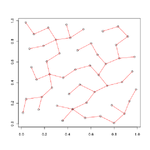
Figure 5: Illustration of two quasi-periodic LHS (left: design with good (large) mindist, right: design with bad (small) mindist).

3.3 Optimization of Latin Hypercube Sample

Within the class of latin hypercube arrangements, optimizing a space-filling criterion in order to avoid undesirable arrangements (such as the diagonal ones which are the worst cases, see also Figure 4) appear very relevant. Optimization can be performed following different approaches, the most natural being the choice of the best LHS (according to the chosen criterion) among a large number (e.g. one thousand). Due to the extremely large number of possible LHS ($(!N)^{d}$ for discretized LHS and infinite for randomized LHS), this method is rather inefficient. Other methods have been developed, based on columnwise-pairwise exchange algorithms, genetic algorithms, Simulated Annealing (SA), etc.: see Viana et al., (2010) for a review. Thus, some practical issues are which algorithm to use to optimize LHS and how to set its numerical parameters. Since an exhaustive benchmark of the available methods (with different parameterizations for the more flexible ones) is hardly possible, we choose to focus on a limited number of specialized stochastic algorithms: the Morris and Mitchell (MM) version of SA (Morris and Mitchell,, 1995), a simple variant of MM developed in Marrel, (2008) (Boussouf algorithm) and a stochastic algorithm called ESE (“Enhanced Stochastic Algorithm”, Jin et al., (2005)). We compare their performance in terms of different space-filling criteria of the resulting designs.

3.3.1 Simulated Annealing (SA)

SA is a probabilistic metaheuristic to solve global optimization problems. The approach can provide a good optimizing point in a large search space. Here, we would like to explore the space of LHS. In fact, the optimization is carried out from an initial LHS (standard random LHS) which is (expected to be) improved through elementary random changes. An elementary change (or elementary perturbation) of a LHS $\mathbf{X}^{N}_{d}$ is done in switching two randomly chosen coordinates from a randomly chosen column, which keeps the latin hypercube nature of the sample. The re-evaluation of the criterion after each elementary change could be very costly (in particular for discrepancy). Yet, taking into account that only two coordinates are involved in an elementary change leads to cheap expressions for the re-evaluation. Formula to re-evaluate in a straightforward way $\phi_{p}$ and the $C^{2}$ discrepancy have been established by Jin et al., (2005). We have extended it to any $L^{2}$-discrepancies (including $W^{2}$ and star $L^{2}$-discrepancy).

The main ideas of SA are the following ones. Designs which do not improve the criterion (bad designs) can be accepted to avoid getting trapped around a local optimum. At each iteration, an elementary change of the current design is proposed, then accepted with a probability which depends on a quantity $T$ called temperature which evolves from an initial temperature $\mathbf{T_{0}}$ according to a certain temperature profile. The temperature decreases with the iterations and less and less bad designs are accepted. The main issue of SA is to properly set the initial temperature and the parameters which define the profile to get a good trade-off between a sufficiently wide exploration of the space and a quick convergence of the algorithm. Finally, a stopping criterion must be specified. The experiments hereafter are stopped when the maximum number of elementary changes is reached, which is useful to compare the different algorithms or to ensure a stop within a chosen duration. However, more sophisticated criteria could be more relevant to save computations or to carry on the optimization while the iterations still result in substantial improvements.

The Boussouf SA algorithm has been introduced in Marrel, (2008). The temperature follows a decreasing geometrical profile: $T=c^{i}\times T_{0}$ at the $i$th iteration with $0<c<1$. Therefore, the temperature decreases exponentially with the iterations and $c$ must be set very close to $1$ when the dimension $d$ is high. In this case, SA can sufficiently explore the LHS designs space if enough iterations are performed and this criterion tends rapidly to a correct approximation of the optimum.

The MM (Morris and Mitchell) SA algorithm (Morris and Mitchell,, 1995) was initially proposed to generate maximin LHS. It can be used to optimize discrepancy criteria, or others as well. Contrary to Boussouf SA, $T$ decreases only if the criterion is not improved during a row of $I_{max}$ iterations. The algorithm stops if the maximum number of elementary changes is reached or if none of the new designs of the last $I_{max}$ iterations has been accepted. Morris & Mitchell proposed some heuristic rules to set the different parameters of the algorithm from $N$ and $d$. We noticed that these rules do not always perform well: some settings can lead to relatively slow convergences.

3.3.2 Enhanced Stochastic Evolutionary algorithm (ESE)

ESE is an efficient and flexible stochastic algorithm for optimizing LHS (Jin et al.,, 2005). It relies on a precise control of a quantity similar to the temperature of SA through an exploration step, then an process of adjustment. ESE behaves as an acceptance-rejection method like SA. ESE is formed from an outer loop and an inner loop. During each of the $M$ iterations of the inner loop, $J$ new LHS are randomly generated from the current one. Then, at each iteration of the outer loop, the temperature is updated via the acceptance ratio; in contrast with SA, it may increase from an (outer) iteration to the next. Finally, during $Q$ iterations of the outer loop, $J\times M\times Q$ elementary design changes are performed. The authors expect ESE to behave more efficiently than SA to optimize LHS.

3.3.3 Feedback on LHS optimization

First, a test is performed to show the performance of the regularization of the mindist criterion (see section 3.2.2). Using ESE, some optimized LHS are produced by means of mindist or $\phi_{p}$; see Figure 6.

mindist

Figure 6: Evolution of the mindist criterion in function of the number of elementary perturbations obtained by ESE ($M=100$, $J=50$) with $\phi_{p}$ (solid line) and mindist (dashed line); ordinates are arithmetic means of the best mindist values from $30$ optimizations of LHS designs ($N=100$, $d=10$).

If the optimizations are performed with $\phi_{p}$ instead of mindist, a clear improvement of mindist is observed. Hence, the $\phi_{p}$ criterion is used in the following to build maximin LHS.

Boussouf SA holds a standard geometric profile which is well-adapted for small values of $d$. When $d$ rises, making a satisfactory choice of $T_{0}$ and $c$ gets more and more difficult. The profile held in MM SA, with $I_{max}\gg 1$ (typically few hundreds), is actually preferable to perform an efficient exploration of the space. Thus, the analysis is focused on MM SA and ESE only in the remainder of this section.

The impact of the parameters as a critical aspect affecting the performances of the algorithms is now considered. Below, the typical behaviour of MM SA for $d\leq 20$ is illustrated. According to our experience, $T_{0}=0.1$ or $0.01$ is a good choice in order not to accept too many bad designs. Then, by a care adjustment of $c$ and $I_{max}$, a trade-off can be found between a relatively fast convergence and the final optimized value of mindist (some larger $I_{max}$ and $c$ for a higher dimension $d$). Figure 7 shows some results with two choices of $I_{max}$ to improve the mindist of a $5$-dimensional LHS of size $N=50$:

• Case $1$ with $T_{0}=0.1$, $I_{max}=100$ and $c=0.9$ (left of Figure 7).

• Case $2$ with $T_{0}=0.1$, $I_{max}=300$ and $c=0.9$ (right of Figure 7).

Figure 7: Maximin LHS designs ($N=50$, $d=5$) obtained by MM SA with $\Phi_{p}$ ($p=50$): comparison and evolution of the mindist as a function of the number of elementary changes. Boxplots are produced from $30$ runs with different initial LHS. Left (case $1$): MM SA with $T_{0}=0.1$, $I_{max}=100$, $c=0.9$. Right (case $2$): MM SA with $T_{0}=0.1$, $I_{max}=300$, $c=0.9$.

MM SA converges faster in case $1$ than in case $2$ (faster flattening of the trajectories) and case $2$ turns out to be a better choice of $I_{max}$ considering the optimization of mindist (greater values when convergence seems achieved).

ESE is now regarded. In a first attempt, the parameters suggested in Jin et al., (2005) are used: see Figure 8.

Figure 8: Maximin LHS design ($N=50$, $d=5$) obtained by ESE ($M=100$ and $J=50$) with $\Phi_{p}$ ($p=50$): comparison and evolution of the mindist criterion as a function of the number of elementary changes. Boxplots are produced from $30$ runs with different initial LHS.

Considering results of case $2$ (right of Figure 7), a faster convergence is obtained with ESE together with similar final optimized values. Indeed, most often, only $15,000$ elementary changes are needed to exceed a mindist of $0.5$ with ESE contrary to what is observed with MM SA in case $2$, which is as efficient as MM SA in case $1$. Thus, ESE combines the convergence speed of MM SA in case $1$ with the ability to find designs of as large mindist as the outcomes from MM SA in case $2$.

Finally, the two following tests are proposed:

• ESE with $M=300$ and $J=50$ (left of Figure 9).

• MM SA with $T_{0}=0.01$, $I_{max}=1000$ and $c=0.98$ (right of Figure 9).

Figure 9: Maximin LHS designs ($N=50$, $d=5$) obtained by ESE and MM SA with $\Phi_{p}$ ($p=50$): comparison and evolution of the mindist criterion as a function of the number of elementary changes. Boxplots are produced through $30$ runs from different initial LHS. Right: MM SA with $T_{0}=0.01$, $I_{max}=1000$ and $c=0.98$. Left: ESE with $M=300$, $J=50$.

Results of ESE and MM SA are similar. Both algorithms cost $350,\!000$ elementary perturbations to exceed $0.56$ which can be considered as a prohibitive budget in comparison with $15,\!000$ to exceed $0.5$ (Figures 7 and 8). Generally, the computational budget required to reach an optimized value $v$ of a discrepancy or point-distance based criterion to maximize (respectively, to minimize) grows much faster than a linear function with respect to $v$ (resp., of $-v$).

Boussouf SA is used in the following section to carry out comparisons of LHS optimizations. This choice enables us to perform many optimizations up to relatively large dimensions within a reasonable duration. If the results cannot be claimed to be perfectly fair due to unfinished optimizations, they are representative of the practice of LHS optimization.

4 Robustness to projections over 2D subspaces

4.1 Motivations

An important characteristic of a SFD $\mathbf{X}_{d}^{N}$ over ${[0;1]}^{d}$ is its robustness to projections over lower-dimensional subspaces, which means that the $k$-dimensional subsamples of the SFD, $k<d$, obtained by deleting $d-k$ columns of the matrix $\mathbf{X}_{d}^{N}$, fill ${[0;1]}^{k}$ efficiently (according to a space filling criterion). A LHS structure for the SFD is not sufficient because it only guarantees good repartitions for one-dimensional projections, and not for projections to subspaces of greater dimensions. Indeed, to capture precisely an interaction effect between some inputs, a good coverage is required onto the subspace spanned by these inputs (see section 2.2).

Another reason why that property of robustness really matters is that a metamodel fitting can be made in a smaller dimension than $d$ (see an example in Cannamela et al., (2008)). In practice, this is often the case because the output analysis of an initial design (“screening step”) may reveal some useless (i.e. non influent) input variables that can be neglected during the metamodel fitting step (Pujol,, 2009). Moreover, when a selection of input variables is made during the metamodel fitting step (as for example in Marrel et al., (2008)), the new sample, solely including the retained input variables, has to keep good space filling properties.

The remainder of the paper is focused on the space filling quality of the 2D projections of optimized LHS. Most of the time, interaction effects of order two (i.e. between two inputs) are significantly larger than interaction of order three, and so on.

Discrepancy and point-distance based criteria can be regarded as relevant measures to quantify the quality of space-filling designs. Unfortunately, they appear incompatible in high dimension in the sense that a quasi-periodic design (see section 3.2.3) does not reach the lowest values of any discrepancy measure (for a LHS of same size $N$). In high dimension, if a discrepancy-optimized LHS is compared to a maximin LHS, some differences between their MST criteria, mean $m$ and standard deviation $\sigma$ (see section 3.2.3), are observed. Moreover, Figure 10 indicates that means $m$, respectively standard deviations $\sigma$, of $C^{2}$-discrepancy optimized LHS are larger, resp. smaller, than ones of $W^{2}$-discrepancy optimized LHS.

Figure 10: MST mean $m$ (left) and standard deviation $\sigma$ (right) of $C^{2}$-discrepancy (solid line) and $W^{2}$-discrepancy (dashed line) optimized LHS of size $N=100$ and dimension $d=10$. Ordinates are arithmetic means of five optimization outcomes.

This is the reason why we will mainly focus on the $C^{2}$-discrepancy rather than the $W^{2}$-discrepancy (in the view of the partial order relation defined in section 3.2.3).

Below, some tests underline the space filling properties of LHS 2D subprojections. Qualities of LHS optimized according to different criteria are analyzed by means of some discrepancies and the MST criteria. All the tests of sections 4.2 and 4.3 are performed with designs of size $N=100$ and of dimension $d$ ranging from $2$ to $54$. To our knowledge, this is the first numerical study with such a range of design dimensions. To capture any variability due to the optimization process, some boxplots are built from all 2D subsamples of five optimized LHS per dimension.

4.2 Analysis according to $L^{2}$-discrepancy measures

Figure 11 displays the $C^{2}$-discrepancies of non-optimized LHS and $C^{2}$-optimized LHS.

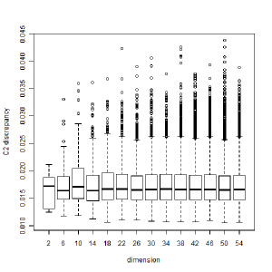
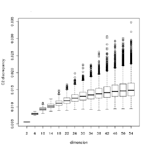
Figure 11: $C^{2}$-discrepancies of the 2D subsamples of non-optimized random LHS (left) and $C^{2}$-discrepancy optimized LHS (right).

The comparison of medians points out that the $C^{2}$-optimized LHS are robust to 2D subprojections in the sense that the 2D subsamples get a reduced $C^{2}$-discrepancy. The optimizations with the $C^{2}$-discrepancy appear efficient for dimensions as large as $54$ since the $C^{2}$-discrepancies of the 2D subsamples are then less than the reference value corresponding to the 2D subsamples of the non-optimized LHS (around $0.017$). This is fully consistent with Fang’s requirement for the so-called modified discrepancies (see section 3.2.1). Moreover, the increase of $C^{2}$-discrepancy (median) of the $C^{2}$-discrepancy optimized LHS with the dimension $d$ is constant and slow. Similar observations can be made with the $W^{2}$-discrepancy instead of the $C^{2}$-discrepancy. Besides, when the same experiment is carried out with the $L^{2}$-star-discrepancy (which is not a modified discrepancy), results are different: see Figure 12.

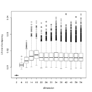
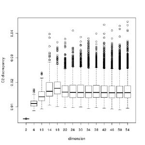
Figure 12: $L^{2}$-star-discrepancies (left) and $C^{2}$-discrepancies (right) of the 2D subsamples of $L^{2}$-star-discrepancy optimized LHS.

In this case, the increase of discrepancy with $d$ is rather fast and the influence of the optimization on 2D subsamples ceases for $d>10$.

Figure 13 illustrates the $C^{2}$-discrepancies of the 2D subsamples of the classical low-discrepancy sequence of Sobol, with Owen scrambling in order to break the alignments created by this deterministic sequence.

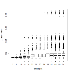
Figure 13: $C^{2}$-discrepancies of the 2D subsamples of the scrambled Sobol’ sequence.

It confirms a well-known fact: the Sobol’ sequence has several poor 2D subprojections in terms of discrepancy, especially in high dimension.

Finally, the same tests are performed on maximin designs. Previous works (Marrel,, 2008; Iooss et al.,, 2010) have shown that maximin designs are not robust in terms of the mindist criterion of their 2D subsamples. It can be explained by alignments in the overall space ${[0;1]}^{d}$. Figure 14 reveals that the maximin design are not robust to projections to 2D subspaces according to two different discrepancies, since results are similar to the ones of the $L^{2}$-star-discrepancy optimized LHS (Figure 12).

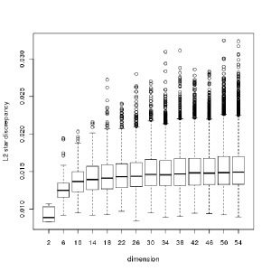
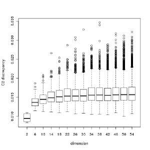
Figure 14: $L^{2}$-star-discrepancies (left) and $C^{2}$-discrepancies (right) of the 2D subsamples of maximin LHS.

It strongly confirms previous conclusions: the maximin design is not recommended if one of the objectives is to have some good space fillings of the 2D subspaces.

4.3 Analysis according to the MST criteria

Due to the lack of robustness of the mindist criterion mentioned in section 3.2.3, only the MST criteria are regarded in the point-distance perspective.

Figure 15 shows that the MST built over the 2D subsamples of maximin LHS have small $m$ and high $\sigma$, even for small dimensions $d$, because of inherent alignments in the entire design.

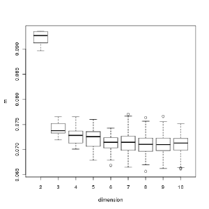
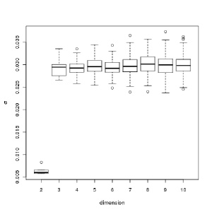
Figure 15: MST mean $m$ (left) and standard deviation $\sigma$ (right) of the 2D subsamples of maximin LHS.

Otherwise, in the case LHS optimized with $C^{2}$-discrepancy, the decrease of $m$ and increase of $\sigma$ for the 2D subsamples are gradual from $d=1$ to $d=10$: see Figure 16.

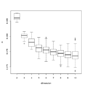
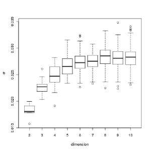
Figure 16: MST mean $m$ (left) and standard deviation $\sigma$ (right) of the 2D subsamples of $C^{2}$-discrepancy optimized LHS

As a consequence, we conclude that $C^{2}$-discrepancy optimized LHS of dimension $d\leq 10$ are less subject than maximin designs to the clustering of points due to projections to 2D subspaces.

5 Discussion and conclusion

5.1 Synthesis of the works

This paper has considered several issues relative to the practice of the building of SFD. Some industrial needs have first been given as challenges: high dimensional SFD are often required (several tens of variables), while preserving good space filling properties on the design subprojections. Several measures of space filling have been discussed: $L^{2}$-discrepancies, mindist interpoint distance criterion (maximin designs), as well as the recently introduced MST criteria. It has been shown that the MST criteria are preferable to the well-known mindist criterion to assess the quality of SFD. The ESE algorithm is shown by our numerical tests to behave more efficiently than the MM SA one, since it generally leads to better improvements of the criterion during the first iterations (for a same number of elementary perturbations) and eventually provides similar final values for large computational durations. Thus, the ESE algorithm appears a relevant choice to carry out LHS optimizations for large dimensions $d$, when restriction on the computational budget is likely to have an impact on the result of optimization. The relevance of the regularized criterion $\phi_{p}$ to compute maximin LHS has also been numerically checked.

Another contribution of this paper is the deep analysis of the space filling properties of the two-dimensional subsamples. Intensive numerical tests have been performed for that purpose, relying on $L^{2}$-discrepancies and minimum spanning tree criteria, with designs of size $N=100$ and of dimension $d$ ranging from $2$ to $54$, which is, to our knowledge, the first numerical study with such a range of design dimensions. Among the tested designs (LHS, maximin LHS, several $L^{2}$-discrepancy optimized LHS, Sobol’ sequence), only the centered ($C^{2}$) and wrap-around ($W^{2}$) discrepancy optimized LHS have shown some strong robustness to 2D projections in high dimension. This result numerically confirms the theoretical considerations of Fang et al., (2006). The other tested designs are not robust to 2D projections when their dimension is larger than $10$. Additional tests, not shown here, on other types of designs, bring the same conclusions.

Table 1 summarizes the main properties of LHS which have been observed.

Table 1: Summary of SFD properties (the second column gives a rank according to the MST partial order relation).

Design	MST	Uniformity on $2$D projections
LHS	$4$	no
maximin LHS	$1$	no
low C$2$-discrepancy LHS	$2$	yes
low W$2$-discrepancy LHS	$3$	yes

Eventually, according to our numerical tests, the best LHS are the $C^{2}$-discrepancy optimized ones, since 2D subprojections are then quite uniform, and, in addition, their MST criteria are better than the ones of the $W^{2}$-discrepancy optimized LHS.

5.2 Feedback on the motivating examples

We illustrate now the benefits achieved by the use of optimized LHS designs on the two motivating examples of section 2.

A typical product of an exploratory study is a metamodel of the computer code from a first set of inputs-outputs (see introduction). In Simpson et al., (2001) and Iooss et al., (2010), several numerical experiments showed the advantage (smaller mean error) of discrepancy-optimized LHS rather than SRS or non-optimized LHS to build an acceptable metamodel. In Marrel and Marquès, (2012), a nuclear safety study involving some accidental scenario simulations was performed using the thermal-hydraulic computer code of section 2.1 ($d=31$ input variables). Because of the high cpu time cost of this code, a metamodel had to be developed. For this purpose, a $W^{2}$-discrepancy optimized LHS of size $N=300$ and the corresponding outputs were computed. The predictivity coefficient of the fitted Gaussian process metamodel (see Fang et al., (2006)) reached $0.87$, which means that $87\%$ of the model output variability was explained by the metamodel. This satisfactory result allowed the authors to use the metamodel to find an interesting set of inputs so as to estimate low quantiles of the model output.

In Iooss et al., (2012), a global sensitivity analysis of the periphyton-grazers sub-model of the prey-predator simulation chain of section 2.2 was carried out. Because of the large number of input variables, Derivative-based Global Sensitivity Measures (DGSM) were used (Lamboni et al.,, 2013). A DGSM is defined as the mean of a square model partial derivative: $\displaystyle\mbox{DGSM}(X_{i})={\mathbb{E}}\left[\left(\frac{\partial G({\mathbf{X}})}{\partial X_{i}}\right)^{2}\right]$. Kucherenko et al., (2009) showed that low-discrepancy sequences are preferable than SRS to estimate DGSM. The partial derivatives of the periphyton-grazers sub-model were computed by finite differences at each point of a $C^{2}$-discrepancy optimized LHS of size $N=100$ and dimension $d=20$. In total, $N\,(d+1)=2100$ model evaluations were performed. A study showed that the estimated DGSM had converged, a result which the SFD directly contributed to.

5.3 Perspectives

As a first perspective, analyses of section 4 could be extended to subprojections of larger dimensions. It is worth noting that, in a preliminary study, Marrel, (2008) confirmed our conclusions about design subprojection properties by considering 3D subsamples.

Another future work would be to carry out a more exhaustive and deeper benchmark of optimization algorithms of LHS. In particular, an idea would be to look at the convergence of the maximin LHS to the exact solutions. These solutions are known in several cases (small $N$ and small $d$) for the non randomized maximin LHS (see van Dam et al., (2007)).

All the SFD of the present work are based on LHS which can be judged as a rather restrictive design structure. Building SFD with good properties in the whole space of possible designs is a grand challenge for future works; see Pronzato and Müller, (2012) for first ideas on this subject.

Finally, lets us note that a complete emphasis has been put on the model input space in this paper which deals with initial exploratory analysis. Of course, the behaviour of the output variables and the objective of the study has generally to be considered afterwards with great caution.

6 Acknowledgments

Part of this work has been backed by French National Research Agency (ANR) through the COSINUS program (project COSTA BRAVA noANR-09-COSI-015). All our numerical tests were performed within the R statistical software environment with the DiceDesign package. We thank Luc Pronzato for helpful discussions and Catalina Ciric for providing the prey-predator model example. Finally, we are grateful to both of the reviewers for their valuable comments and their help with the English.

References

- Auder et al., (2012) Auder, B., de Crécy, A., Iooss, B., and Marquès, M. (2012). Screening and metamodeling of computer experiments with functional outputs. Application to thermal-hydraulic computations. Reliability Engineering and System Safety, 107:122–131.
- Cannamela et al., (2008) Cannamela, C., Garnier, J., and Iooss, B. (2008). Controlled stratification for quantile estimation. Annals of Apllied Statistics, 2:1554–1580.
- Cheng and Davenport, (1989) Cheng, R. and Davenport, T. (1989). The problem of dimensionality in stratified sampling. Management Science, 35:1278–1296.
- Ciric et al., (2012) Ciric, C., Ciffroy, P., and Charles, S. (2012). Use of sensitivity analysis to discriminate non-influential and influential parameters within an aquatic ecosystem model. Ecological Modelling, 246:119–130.
- de Crécy et al., (2008) de Crécy, A., Bazin, P., Glaeser, H., Skorek, T., Joucla, J., Probst, P., Fujioka, K., Chung, B., Oh, D., Kyncl, M., Pernica, R., Macek, J., Meca, R., Macian, R., D’Auria, F., Petruzzi, A., Batet, L., Perez, M., and Reventos, F. (2008). Uncertainty and sensitivity analysis of the LOFT L2-5 test: Results of the BEMUSE programme. Nuclear Engineering and Design, 12:3561–3578.
- de Rocquigny et al., (2008) de Rocquigny, E., Devictor, N., and Tarantola, S., editors (2008). Uncertainty in industrial practice. Wiley.
- Dussert et al., (1986) Dussert, C., Rasigni, G., Rasigni, M., and Palmari, J. (1986). Minimal spanning tree: A new approach for studying order and disorder. Physical Review B, 34(5):3528–3531.
- Fang, (2001) Fang, K.-T. (2001). Wrap-around -discrepancy of random sampling, Latin hypercube and uniform designs. Journal of Complexity, 17:608–624.
- Fang et al., (2006) Fang, K.-T., Li, R., and Sudjianto, A. (2006). Design and modeling for computer experiments. Chapman & Hall/CRC.
- Fang and Lin, (2003) Fang, K.-T. and Lin, D. K. (2003). Uniform experimental designs and their applications in industry. Handbook of Statistics, 22:131–178.
- Franco, (2008) Franco, J. (2008). Planification d’expériences numériques en phase exploratoire pour la simulation des phénomènes complexes. Thèse de l’Ecole Nationale Supérieure des Mines de Saint-Etienne, France.
- Franco et al., (2008) Franco, J., Bay, X., Corre, B., and Dupuy, D. (2008). Strauss processes: A new space-filling design for computer experiments. In Proceedings of Joint Meeting of the Statistical Society of Canada and the Société Française de Statistique, Ottawa, Canada.
- Franco et al., (2009) Franco, J., Vasseur, O., Corre, B., and Sergent, M. (2009). Minimum spanning tree: A new approach to assess the quality of the design of computer experiments. Chemometrics and Intelligent Laboratory Systems, 97:164–169.
- Gentle, (2003) Gentle, J. (2003). Random number generation and Monte Carlo methods. Springer.
- (15) Hickernell, F. (1998a). A generalized discrepancy and quadrature error bound. Mathematics of Computation, 67:299–322.
- (16) Hickernell, F. (1998b). Lattice rules: how well do they measure up? In Hellekalek, P. and Larcher, G., editors, Random and quasi-random point sets, pages 106–166. Springer-Verlag Berlin/New-York.
- Iooss et al., (2010) Iooss, B., Boussouf, L., Feuillard, V., and Marrel, A. (2010). Numerical studies of the metamodel fitting and validation processes. International Journal of Advances in Systems and Measurements, 3:11–21.
- Iooss et al., (2012) Iooss, B., Popelin, A.-L., Blatman, G., Ciric, C., Gamboa, F., Lacaze, S., and Lamboni, M. (2012). Some new insights in derivative-based global sensitivity measures. In Proceedings of the PSAM11 ESREL 2012 Conference, pages 1094–1104, Helsinki, Finland.
- Jin et al., (2005) Jin, R., Chen, W., and Sudjianto, A. (2005). An efficient algorithm for constructing optimal design of computer experiments. Journal of Statistical Planning and Inference, 134:268–287.
- Johnson et al., (1990) Johnson, M., Moore, L., and Ylvisaker, D. (1990). Minimax and maximin distance design. Journal of Statistical Planning and Inference, 26:131–148.
- Kleijnen and Sargent, (2000) Kleijnen, J. and Sargent, R. (2000). A methodology for fitting and validating metamodels in simulation. European Journal of Operational Research, 120:14–29.
- Koehler and Owen, (1996) Koehler, J. and Owen, A. (1996). Computer experiments. In Ghosh, S. and Rao, C., editors, Design and analysis of experiments, volume 13 of Handbook of statistics. Elsevier.
- Kucherenko et al., (2009) Kucherenko, S., Rodriguez-Fernandez, M., Pantelides, C., and Shah, N. (2009). Monte carlo evaluation of derivative-based global sensitivity measures. Reliability Engineering and System Safety, 94:1135–1148.
- Lamboni et al., (2013) Lamboni, M., Iooss, B., Popelin, A.-L., and Gamboa, F. (2013). Derivative-based global sensitivity measures: general links with sobol’ indices and numerical tests. Mathematics and Computers in Simulation, 87:45–54.
- Lemieux, (2009) Lemieux, C. (2009). Monte Carlo and quasi-Monte Carlo sampling. Springer.
- Loeppky et al., (2009) Loeppky, J., Sacks, J., and Welch, W. (2009). Choosing the sample size of a computer experiment: A practical guide. Technometrics, 51:366–376.
- Marrel, (2008) Marrel, A. (2008). Mise en oeuvre et exploitation du métamodèle processus gaussien pour l’analyse de modèles numériques - Application à un code de transport hydrogéologique. Thèse de l’INSA Toulouse, France.
- Marrel et al., (2009) Marrel, A., Iooss, B., Laurent, B., and Roustant, O. (2009). Calculations of the Sobol indices for the Gaussian process metamodel. Reliability Engineering and System Safety, 94:742–751.
- Marrel et al., (2008) Marrel, A., Iooss, B., Van Dorpe, F., and Volkova, E. (2008). An efficient methodology for modeling complex computer codes with Gaussian processes. Computational Statistics and Data Analysis, 52:4731–4744.
- Marrel and Marquès, (2012) Marrel, A. and Marquès, M. (2012). Sensitivity analysis of safety factor predictions for nuclear component behaviour under accidental conditions. In Proceedings of the PSAM11 ESREL 2012 Conference, pages 1134–1143, Helsinki, Finland.
- McKay et al., (1979) McKay, M., Beckman, R., and Conover, W. (1979). A comparison of three methods for selecting values of input variables in the analysis of output from a computer code. Technometrics, 21:239–245.
- Morris and Mitchell, (1995) Morris, M. and Mitchell, T. (1995). Exploratory designs for computationnal experiments. Journal of Statistical Planning and Inference, 43:381–402.
- Niederreiter, (1987) Niederreiter, H. (1987). Low-discrepancy and low-dispersion sequences. Journal of Number Theory, 30:51–70.
- Park, (1994) Park, J.-S. (1994). Optimal Latin-hypercube designs for computer experiments. Journal of Statistical Planning and Inference, 39:95–111.
- Pronzato and Müller, (2012) Pronzato, L. and Müller, W. (2012). Design of computer experiments: space filling and beyond. Statistics and Computing, 22:681–701.
- Pujol, (2009) Pujol, G. (2009). Simplex-based screening designs for estimating metamodels. Reliability Engineering and System Safety, 94:1156–1160.
- Sacks et al., (1989) Sacks, J., Welch, W., Mitchell, T., and Wynn, H. (1989). Design and analysis of computer experiments. Statistical Science, 4:409–435.
- Saltelli et al., (2006) Saltelli, A., Ratto, M., Tarantola, S., and Campolongo, F. (2006). Sensitivity analysis practices: Strategies for model-based inference. Reliability Engineering and System Safety, 91:1109–1125.
- Santner et al., (2003) Santner, T., Williams, B., and Notz, W. (2003). The design and analysis of computer experiments. Springer.
- Schwery and Wynn, (1987) Schwery, M. and Wynn, H. (1987). Maximum entropy sampling. Journal of Applied Statistics, 14:165–170.
- Simpson et al., (2001) Simpson, T., Lin, D., and Chen, W. (2001). Sampling strategies for computer experiments: Design and analysis. International Journal of Reliability and Applications, 2:209–240.
- van Dam et al., (2007) van Dam, E., Husslage, B., den Hertog, D., and Melissen, H. (2007). Maximin Latin hypercube designs in two dimensions. Operations Research, 55:158–169.
- Varet et al., (2012) Varet, S., Lefebvre, S., Durand, G., Roblin, A., and Cohen, S. (2012). Effective discrepancy and numerical experiments. Computer Physics Communications, 183:2535–2541.
- Viana et al., (2010) Viana, F., Venter, G., and Balabanov, V. (2010). An algorithm for fast optimal Latin hypercube design of experiments. International Journal for Numerical Methods in Engineering, 82:135–156.