Asymptotic behaviour of solutions to the stationary
Navier-Stokes equations in two dimensional exterior domains
with zero velocity at infinity

Abstract

We investigate analytically and numerically the existence of stationary solutions converging to zero at infinity for the incompressible Navier-Stokes equations in a two-dimensional exterior domain. More precisely, we find the asymptotic behaviour for such solutions in the case where the net force on the boundary of the domain is non-zero. In contrast to the three dimensional case, where the asymptotic behaviour is given by a scale invariant solution, the asymptote in the two-dimensional case is not scale invariant and has a wake. We provide an asymptotic expansion for the velocity field at infinity, which shows that, within a wake of width $|\boldsymbol{x}|^{2/3}$, the velocity decays like $|\boldsymbol{x}|^{-1/3}$, whereas outside the wake, it decays like $|\boldsymbol{x}|^{-2/3}$. We check numerically that this behaviour is accurate at least up to second order and demonstrate how to use this information to significantly improve the numerical simulations. Finally, in order to check the compatibility of the present results with rigorous results for the case of zero net force, we consider a family of boundary conditions on the body which interpolate between the non-zero and the zero net force case.

Keywords: Navier-Stokes equations, Flow-structure interactions, Wakes, Computational methods
MSC class: 76D03, 76D05, 35Q30, 76D10, 76D25, 74F10, 76M10

1 Introduction

In what follows, we discuss the question of the existence of solutions for the incompressible Navier-Stokes equations in the exterior domain $\Omega=\mathbb{R}^{2}\setminus B(\boldsymbol{0},1)$ where $B(\boldsymbol{0},1)$ is the closed disk of radius one centred at the origin,

$$\Delta\boldsymbol{u}-\boldsymbol{\nabla}p =\boldsymbol{u}\boldsymbol{\cdot}\boldsymbol{\nabla}\boldsymbol{u}\,, \boldsymbol{\nabla}\boldsymbol{\cdot}\boldsymbol{u} =0\,,$$ (1a)

$$\left.\boldsymbol{u}\right|_{\partial B(\boldsymbol{0},1)} =\boldsymbol{u}^{*}\,, \lim_{|\boldsymbol{x}|\to\infty}\boldsymbol{u} =\boldsymbol{0}\,,$$

where $$\boldsymbol{u}^{*}$$ is any smooth boundary condition with no net flux,

$$\int_{\partial B(\boldsymbol{0},1)}\boldsymbol{u}^{*}\boldsymbol{\cdot}\boldsymbol{n}=0\,.$$ (1b)

In these equations, $\boldsymbol{u}$ is the velocity field, $p$ the pressure and $\boldsymbol{n}$ the outward normal unit vector to the body $B(\boldsymbol{0},1)$. By using the scaling symmetry of the Navier-Stokes equations, this also covers the case of a disk of arbitrary size. Also, our results are very likely not changed if one replaces the disk with an arbitrary bounded domain with a smooth enough boundary. We define the net force $\boldsymbol{F}$ and the torque $M$ acting on the body by

$$\boldsymbol{F} =\int_{\partial B(\boldsymbol{0},1)}\mathbf{T}\boldsymbol{n}\,, M =\int_{\partial B(\boldsymbol{0},1)}\boldsymbol{x}\boldsymbol{\wedge}\mathbf{T}\boldsymbol{n}\,,$$ (2)

where $\mathbf{T}$ is the stress tensor including the convective part, $\mathbf{T}=\boldsymbol{u}\otimes\boldsymbol{u}+p-\boldsymbol{\nabla}\boldsymbol{u}-\left(\boldsymbol{\nabla}\boldsymbol{u}\right)^{T}$. The net force and the torque are the two conserved quantities of the Navier-Stokes equations, in the sense that (2) is invariant if one replaces $\partial B(\boldsymbol{0},1)$ by any homotopic smooth curve. In particular the curve can be pushed to infinity, so that these two quantities are encoded in the behaviour of the solution at infinity, which plays an important role below.

Problem (1b) is closely related to the one of the incompressible Navier-Stokes equations in $\mathbb{R}^{2}$,

$$\Delta\boldsymbol{u}-\boldsymbol{\nabla}p =\boldsymbol{u}\boldsymbol{\cdot}\boldsymbol{\nabla}\boldsymbol{u}-\boldsymbol{f}\,, \boldsymbol{\nabla}\boldsymbol{\cdot}\boldsymbol{u} =0\,, \lim_{|\boldsymbol{x}|\to\infty}\boldsymbol{u} =\boldsymbol{0}\,,$$ (3)

where the force term $\boldsymbol{f}$ is a smooth function of compact support. See for example Hillairet & Wittwer (2012) where the connection between two such problems is made precise. For problem (3), the net force $\boldsymbol{F}$ and the torque $M$ are defined by

$$\boldsymbol{F} =\int_{\mathbb{R}^{2}}\boldsymbol{f}\,, M =\int_{\mathbb{R}^{2}}\boldsymbol{x}\boldsymbol{\wedge}\boldsymbol{f}\,.$$ (4)

Even for small data $\boldsymbol{u}^{*}$ or $\boldsymbol{f}$, it is an open question if problems (1b) and (3) admit a solution for general data (see Galdi, 2011, 2004, for a complete review of the question), and the resolution of this question is one of the most challenging open mathematical problems of two-dimensional stationary fluid mechanics (Yudovich, 2003). The main difficulty is to determine the behaviour of solutions at infinity: the existence of so-called $D$-solutions for the Navier-Stokes equations is a well-known result, but the function spaces used in these proofs are not sufficiently restrictive to prove that the velocity goes to zero at infinity.

The difficulty of proving that the boundary condition at infinity is satisfied is specific to the two-dimensional stationary Navier-Stokes equations with zero velocity at infinity (see Galdi, 2011, notes on §XII.5). More precisely, this difficulty is related to the fact that the linearisation around zero of the Navier-Stokes equation is the Stokes equation, and it is known that solutions of the Stokes equation in two-dimensions do in general not decay at infinity. This fact is known as the Stokes paradox. If solutions to the Navier-Stokes equations do exist, their asymptotic behaviour can therefore not in general be given by a solution of the Stokes equation, and this is why the question of the existence of such solutions relies heavily on guessing the correct asymptotic behaviour.

We note that the problem which one obtains when the boundary condition at infinity is replaced by a non-zero constant vector field is completely different from the one considered here (Finn & Smith, 1967). The linearisation around the constant vector field at infinity leads to the Oseen equation which, in contrast to the Stokes equation, possesses a fundamental solution which decays to zero at infinity. Therefore, a fixed point argument can be used in that case (Galdi & Sohr, 1995; Sazonov, 1999), and the solution of the Navier-Stokes equations is asymptotic at infinity to the Oseen fundamental solution.

In three dimensions, the situation is somewhat similar, since there is also a fundamental distinction between the case where the velocity at infinity is zero, or a non-zero constant vector field. However, in contrast to the two-dimensional case, the functions spaces used for the construction of $D$-solutions ensure in three dimensions that the velocity converges to the prescribed value at infinity (see Galdi, 2011, §X.4). For a non-zero constant vector field at infinity, the relevant linear problem is again the Oseen equation and the asymptotic behaviour of the velocity is given by the Oseen fundamental solution (Finn, 1959; Babenko, 1973; Galdi, 1992; Farwig & Sohr, 1998). In the case of zero velocity at infinity, Galdi (1993) proves that the solution decays at infinity as $|\boldsymbol{x}|^{-1}$, i.e. like the fundamental solution of the three-dimensional Stokes equation. The solution, nevertheless, does not admit the Stokes fundamental solution as its asymptote (Deuring & Galdi, 2000). The reason for this is that a solution decaying like $|\boldsymbol{x}|^{-1}$ makes the linear term of the Navier-Stokes equation, $\Delta\boldsymbol{u}$, and the non-linear one, $\boldsymbol{u}\boldsymbol{\cdot}\boldsymbol{\nabla}\boldsymbol{u}$, having both the same decay like $|\boldsymbol{x}|^{-3}$. Recently Nazarov & Pileckas (1999, 2000) showed that the asymptotic behaviour is given by a self-similar solution decaying like $|\boldsymbol{x}|^{-1}$, and Korolev & Šverák (2011) then proved that the asymptotic behaviour coincides with solutions of the Navier-Stokes equations in $\mathbb{R}^{3}\setminus\left\{\boldsymbol{0}\right\}$ found by Landau (Landau, 1944). The family of Landau solutions depends on one real parameter which is related to the net force, and therefore the asymptote encodes the information concerning the net force at infinity. In two dimensions, the analogous self-similar solutions are given by Hamel solutions (Hamel, 1917), but in contrast to the three-dimensional case, the Hamel solutions depend on a discrete parameter, and therefore cannot encode the net force at infinity. Indeed, Šverák (2011, §5) proves that the asymptote in two dimensions cannot be a self-similar solution and in particular that one cannot obtain a solution to (3) with perturbation techniques in a space a functions that decay like $O(|\boldsymbol{x}|^{-1})$ at infinity. In any case, solutions decaying like $O(|\boldsymbol{x}|^{-1})$ at infinity decay too fast to encode a non-zero net force at infinity.

For all these reasons, the two-dimensional case with zero velocity at infinity is particularly difficult and remains the only stationary case where the existence of solutions satisfying the boundary condition at infinity is not known for general data. A few results are available under symmetry assumptions on the data, by Galdi (2004, §3.3) and by Russo (2008, §4.4) for the body case (1b), and by Yamazaki (2009) for the case of a force (3). Pileckas & Russo (2012) also consider symmetric boundary conditions, but allow a non-zero net flux through the boundary. In all cases, the symmetry assumptions imply either a zero net force on the boundary or a zero mean of the force $\boldsymbol{f}$. Recently, Hillairet & Wittwer (2013) proved the existence of solutions decaying like $|\boldsymbol{x}|^{-1}$ for a ball of boundary conditions that are not centred at zero; more precisely the ball is centred on the non-slip boundary condition corresponding to a rotating body.

Note that the analogy between the problem (1b) and (3) is at a formal level only, since in order to make the analogy precise, existence and uniqueness of solutions needs to be known in both cases. Formally, to pass from a solution for the source force case (3) to a solution of the body case (1b), one simply evaluates the solution $\boldsymbol{u}$ on $\partial\Omega$ which provides the corresponding $\boldsymbol{u}^{*}$ (we assume here that $\operatorname{supp}\boldsymbol{f}\subset B(\boldsymbol{0},1)$, which can always been achieved by the scale invariance of the Navier-Stokes equations). Conversely, one can cutoff the stream function of the body problem to obtain a solution in the whole space with a source force. In this step, the relation (1b) is crucial to ensure that the stream function in the exterior domain exists globally. As mentioned above, the equivalence has been proven for an analogue problem with constant velocity at infinity (Hillairet & Wittwer, 2012).

The present work, is a first step towards solving the open problems (1b) and (3) for the case of a non-zero net force $\boldsymbol{F}$. Guided by related problems (van Dyke, 1975) and in particular by the semi-infinite plate problem (Goldstein, 1957; Ockendon & Ockendon, 1995; Bichsel & Wittwer, 2007), we look for an asymptotic expansion describing the asymptotic behaviour at large distances from the origin. As explained below, the Navier-Stokes equations together with the condition of a non-zero net force fixes the decay of the velocity within the wake: if the decay is too slow, the force is infinite, and if the decay is too fast, the force is zero. Moreover, we show below that the requirement of the torque to be finite implies that the first two orders of the asymptotic expansion are symmetric with respect to an axis aligned in the direction the net force $\boldsymbol{F}$. We have the following conjecture:

Conjecture 1.

For a large class of boundary conditions $\mathbf{u}^{*}$ (resp. source terms $\boldsymbol{f}$) with a non-zero net force $\boldsymbol{F}$, there exists a solution to (2) (resp. to (3)) which satisfies

$$u =u_{0}+u_{1}+O(r^{-1})\,, p =p_{0}+p_{1}+O(r^{-2})\,,$$

$$v =v_{0}+v_{1}+O(r^{-4/3})\,, \omega =\omega_{0}+\omega_{1}+O(r^{-5/3})\,,$$

where $\boldsymbol{u}=\left(u,v\right)$, $\omega=\boldsymbol{\nabla}\boldsymbol{\wedge}\boldsymbol{u}$, and $r=|\boldsymbol{x}|$. For $i\in\left\{0,1\right\}$, the functions defining the asymptotic behaviour satisfy $u_{i}=O(r^{-(1+i)/3})$, $v_{i}=O(r^{-(2+i)/3})$, $p_{i}=O(r^{-(4+i)/3})$ and $\omega_{i}=O(r^{-(3+i)/3})$, and moreover depend only on the net force $\boldsymbol{F}$. In a coordinate system where $\boldsymbol{F}=\left(F,0\right)$ with $F>0$, the asymptotes are given explicitly, for $i=0$, by (15d) with $b_{0}=0$, and, for $i=1$, by (18d) with $b_{1}=0$. The parameter $a$ in the asymptotes is linked to the net force $F$ through (19).

In order to check that the asymptotic expansion at first (15d) and second (18d) order describes the behaviour at infinity correctly, we solve the problem numerically on truncated domains of increasing size and look at the decay of the horizontal velocity $u$ up-stream and down-stream along the $x$-axis, as well as at the profile of $u$ and $\omega$ in the $y$-direction at fixed values of $x$. We then show that the knowledge of the asymptotic behaviour can significantly improve the numerical simulations, by using the asymptotic terms to define an artificial boundary condition (Bönisch et al., 2005; Boeckle & Wittwer, 2013). Finally, in view of the solutions found by Hillairet & Wittwer (2013) we study the transition from the case of non-zero net force to zero force, by varying the boundary condition on the body appropriately.

2 Asymptotic expansion

In this section, we limit the discussion to problem (3) of a force of compact support, since the analysis is identical for problem (1b). We only treat the case where the net force $\boldsymbol{F}$ defined by (4) is different from zero. Without loss of generality we choose the orientation of the coordinates $\boldsymbol{x}=\left(x,y\right)$ such that $\boldsymbol{F}=\left(F,0\right)$, with $F>0$. Moreover, modulo a translation in the $y$-direction, we can always choose the coordinates such that the torque $M$ defined in (4) is zero, $M=0$.

In order to simplify the calculations, we choose to work with the vorticity equation,

$$\Delta\omega-\boldsymbol{u}\boldsymbol{\cdot}\boldsymbol{\nabla}\omega =-\boldsymbol{\nabla}\boldsymbol{\wedge}\boldsymbol{f}\,, \boldsymbol{\nabla}\boldsymbol{\cdot}\boldsymbol{u} =0\,,$$ (5)

where $\omega=\boldsymbol{\nabla}\boldsymbol{\wedge}\boldsymbol{u}$ is the vorticity, since that way the pressure is eliminated. The incompressible vorticity equation (5) reduces to a partial differential equation of order four for the stream function $\psi$, which is defined by $\boldsymbol{u}=\boldsymbol{\nabla}\wedge\psi$. Once the stream function as been determined, we can construct the pressure $p$ by integrating, for example, the second component of the Navier-Stokes equation with respect to $y$. In what follows, we use the stream function as the fundamental quantity in order to find the asymptotic behaviour: we make an Ansatz for the stream function which includes a wake, find the correct parameters of the wake based on physical arguments and compute the first two leading terms of the expansion.

Since the net force is oriented along the $x$-axis, it is natural to discuss the symmetries of the Navier-Stokes equations (3) with respect to the horizontal axis. It is well known that the equation for the stream function is invariant under the symmetry given by $\psi(x,y)=-\psi(x,-y)$, provided that the force satisfies $\boldsymbol{f}(x,y)=\operatorname{diag}(1,-1)\boldsymbol{f}(x,-y)$, which in (3) corresponds to the symmetry, $\boldsymbol{u}(x,y)=\operatorname{diag}(1,-1)\boldsymbol{u}(x,-y)$ and $p(x,y)=-p(x,-y)$. Such solutions will be called symmetric in what follows.

2.1 Wake parameters

Since $F>0$, it is natural (see Goldstein, 1957; van Dyke, 1975; Bichsel & Wittwer, 2007; Bönisch et al., 2008) to look for a wake region in the half-plane characterized by $x>0$ with a wake variable defined by $z=y/x^{p}$, where $0<p<1$. We first consider only the wake region $x>0$, where in all known cases the velocity field has the slowest decay. Below we then construct the stream function in the whole plane by multiplying the functions describing the wake by a Heaviside function $H(x)$, and by adding a harmonic function to restore all the boundary conditions (see Goldstein, 1957; Bichsel & Wittwer, 2007). We start with the following Ansatz for the dominant term of the stream function in the wake, i.e. for large $x$ at fixed $z$,

$$\psi(x,y)\approx x^{q}\varphi_{0}(z)+o(x^{q})\,,$$

where $0<p<1$ and $q\in\mathbb{R}$. Under the usual assumptions concerning the differentiability of the asymptotic expansion (Goldstein, 1957; van Dyke, 1975), the velocity field $\boldsymbol{u}=\left(u,v\right)$ and the vorticity $\omega=\boldsymbol{\nabla}\boldsymbol{\wedge}\boldsymbol{u}$ admit the expansions

$$u(x,y) =x^{q-p}\varphi_{0}^{\prime}(z)+o(x^{q-p})\,,$$

$$v(x,y) =x^{q-1}\left(pz\varphi_{0}^{\prime}(z)-q\varphi_{0}(z)\right)+o(x^{q-1})\,,$$

$$\omega(x,y) =-x^{q-2p}\varphi_{0}^{\prime\prime}(z)+o(x^{q-2p})\,.$$

By plugging this Ansatz into the equation for the vorticity we obtain

$$\Delta\omega-\boldsymbol{u}\boldsymbol{\cdot}\boldsymbol{\nabla}\omega=-x^{q-4p}\varphi_{0}^{(4)}(z)-x^{2q-3p-1}\left(q\varphi_{0}(z)\varphi_{0}^{(3)}(z)+\left(2p-q\right)\varphi_{0}^{\prime}(z)\varphi_{0}^{\prime\prime}(z)\right)+o(x^{\max(q-4p,2q-3p-1)})\,.$$ (6)

In order to obtain a differential equation for the wake involving the linear and non-linear part of the Navier-Stokes equation, we have to choose

$$q-4p=2q-3p-1\qquad\Longleftrightarrow\qquad p+q=1\,.$$ (7)

With this condition the vorticity equation becomes

$$\Delta\omega-\boldsymbol{u}\boldsymbol{\cdot}\boldsymbol{\nabla}\omega=-x^{1-5p}\left(\varphi_{0}^{(4)}(z)+\left(1-p\right)\varphi_{0}(z)\varphi_{0}^{(3)}(z)+\left(3p-1\right)\varphi_{0}^{\prime}(z)\varphi_{0}^{\prime\prime}(z)\right)+o(x^{1-5p})\,.$$ (8)

Since we are interested in a solution that provides a net force, we need to satisfy the equation

$$\boldsymbol{F}=\left(F,0\right)=\lim_{R\to\infty}\lim_{S\to\infty}\int_{\partial\left(\left[-R,R\right]\times\left[-S,S\right]\right)}\mathbf{T}\boldsymbol{n}\,,$$ (9)

where $\mathbf{T}$ is the stress tensor including the convective part. By assuming that the pressure and the velocity outside the wake do not influence the net force, a fact that will be verified later on, we find

$$\boldsymbol{F}=\left(F,0\right)=\lim_{x\to\infty}\int_{-\infty}^{+\infty}\boldsymbol{u}u\,\mathrm{d}y=\lim_{x\to\infty}\left[\int_{-\infty}^{+\infty}\left(x^{2q-p}\varphi_{0}^{\prime}(z)^{2},0\right)\mathrm{d}z+o(x^{2q-p})\right]\,.$$ (10)

In order to obtain a finite non-zero net force we therefore have to choose $p$ and $q$ such that $2q-p=0$, which together with the relation (7) fixes the exponents,

$$p =\frac{2}{3}\,, q =\frac{1}{3}\,,$$ (11)

and from (10) we therefore get that the net force is related to the function $\varphi_{0}$ by

$$F=\int_{-\infty}^{+\infty}\varphi_{0}^{\prime}(z)^{2}\mathrm{d}z\,.$$ (12)

The previous analysis demonstrates that the stream function $\psi=x^{1/3}\varphi_{0}(z)$ with $\varphi_{0}$ the solution of the differential equation appearing in the right hand side of (8), satisfies the vorticity equation (8) in the wake with a remainder of order $O(x^{-8/3})$ for large $x$ at fixed $z$. The aim of the asymptotic expansion which we construct now is to improve the decay of the remainder at each step of the development. In view of (6) and by requiring that the terms generated by the previous orders cancel in the wake, the natural Ansatz for the stream function in the wake is

$$\psi=x^{1/3}\varphi_{0}(z)+\varphi_{1}(z)+x^{-1/3}\varphi_{2}(z)+\cdots\,,$$ (13)

where $z=y/x^{2/3}$ is the wake variable. By plugging this Ansatz into the vorticity equation (5), the terms of order $x^{-(7+i)/3}$ define an ordinary differential equation for $\varphi_{i}$. Consequently, the asymptotic expansion is in powers of $x^{-1/3}$, eventually with logarithmic corrections entering the expansion at some point (see for example Bönisch et al., 2008, §2). In the following we solve these differential equations for the first two orders, and extend the asymptotic expansion from the wake region to the whole plane by using techniques from harmonic analysis.

2.2 First order term

With $p$ and $q$ fixed by (11), the function $\varphi_{0}$ has to satisfy the differential equation obtained from (8),

$$\varphi_{0}^{(4)}+\frac{1}{3}\varphi_{0}\,\varphi_{0}^{(3)}+\varphi_{0}^{\prime}\,\varphi_{0}^{\prime\prime}=0\,.$$

After three explicit integrations, the equation becomes

$$\varphi_{0}^{\prime}+\frac{1}{6}\varphi_{0}^{2}=C_{2}z^{2}+C_{1}z+C_{0}\,,$$

where $C_{0},C_{1},C_{2}\in\mathbb{R}$ are some constants. The derivative $\varphi_{0}^{\prime}$ has to be zero at infinity so that the horizontal velocity $u$ satisfies the boundary condition (1a) at infinity, and the requirement that the velocity field is bounded implies that $\varphi_{0}$ is bounded. This is only possible if $C_{1}=C_{2}=0$, and consequently, the resulting bounded solutions are given explicitly by

$$\varphi_{0}(z)=6a\tanh(az-b_{0})\,,$$ (14)

where $a>0$ is a constant related to $C_{0}$ by $C_{0}=6a^{2}$, and $b_{0}\in\mathbb{R}$. The parameter $b_{0}$ introduces symmetry breaking, since for $b_{0}=0$, the stream function defined above corresponds to a symmetric solution, whereas for $b_{0}\neq 0$, the solution is not symmetric. At the end of this subsection, we show that $b_{0}=0$, since otherwise the torque would be infinite. We note that $\varphi_{0}^{\prime}$ decays exponential fast at infinity, and that $\varphi_{0}$ is bounded but does not converge to zero at infinity. Therefore, as in the semi-infinite plate case (Goldstein, 1957; Bichsel & Wittwer, 2007), the horizontal component $u$ satisfies the boundary condition at infinity, but $v$ does not go to zero at infinity for fixed $x$,

$$\lim_{y\to\pm\infty}u(x,y) =\frac{1}{x^{1/3}}\lim_{z\to\pm\infty}\varphi_{0}^{\prime}(z)=0\,,$$

$$\lim_{y\to\pm\infty}v(x,y) =\frac{1}{3x^{2/3}}\lim_{z\to\pm\infty}\left(2z\varphi_{0}^{\prime}(z)-\varphi_{0}(z)\right)=\frac{\mp 1}{3x^{2/3}}\,.$$

Following Goldstein (1957) and others (van Dyke, 1975; Bichsel & Wittwer, 2007), in order to restore the boundary condition for $v$, we introduce a branch-cut along the positive real axis, subtract from $\varphi_{0}(z)$ its asymptote at large $z$, i.e. $6a\operatorname{sign}z$, and compensate the resulting discontinuity on the branch-cut by adding to the stream function an appropriate harmonic function. Explicitly we take

$$\psi_{0}=H(x)x^{1/3}\left(\varphi_{0}(z)-6a\operatorname{sign}z\right)-4\sqrt{3}ar^{1/3}\sin(\theta/3)\,,$$

where $H$ is the Heaviside function, $r=\sqrt{x^{2}+y^{2}}$ and $\theta=\arg\left(-x-\mathrm{i}y\right)$ is the angle measured from the negative real axis. That way, and since $\varphi_{0}(z)-6a\operatorname{sign}z$ decays exponential fast at infinity, the term multiplied by $H(x)$ and the harmonic term are smooth in $\mathbb{R}^{2}\setminus\left[0,\infty\right)$ and the resulting velocity field decays at infinity. Moreover, the function $\psi_{0}$ is by construction continuous across the branch-cut and therefore continuous in the whole plane apart from the origin. By adding higher order terms to $\psi_{0}$, one could obtain a stream function which is arbitrarily smooth away from the origin. For simplicity these terms are not written here, since they do not change the following argument in any way. The first order of the velocity field and of the vorticity are

$$u_{0} =\frac{H(x)}{x^{1/3}}\varphi_{0}^{\prime}(z)-\frac{4a}{\sqrt{3}}\frac{x\cos(\theta/3)+y\sin(\theta/3)}{r^{5/3}}\,,$$ (15a)

$$v_{0} =\frac{H(x)}{3x^{2/3}}\left(2z\varphi_{0}^{\prime}(z)-\varphi_{0}(z)+6a\operatorname{sign}z\right)+\frac{4a}{\sqrt{3}}\frac{x\sin(\theta/3)-y\cos(\theta/3)}{r^{5/3}}\,,$$ (15b)

$$\omega_{0} =-\frac{H(x)}{x}\varphi_{0}^{\prime\prime}(z)\,.$$ (15c)

Finally, by integrating the second component of the Navier-Stokes equation with respect to $$y$$, and requiring that the pressure is zero at infinity, we reconstruct the pressure term at leading order,

$$p_{0}=\frac{H(x)}{x^{4/3}}\frac{4a^{2}}{3}\left(\rho_{0}(z)-4b_{0}\operatorname{sign}z\right)+\frac{8a^{2}}{3r^{4/3}}+\frac{32a^{2}b_{0}}{3\sqrt{3}}\frac{\sin(4\theta/3)}{r^{4/3}}\,,$$ (15d)

where

$$\rho_{0}(z)=4az\tanh(az-b_{0})-4\log(2\cosh(az-b_{0}))+2az\tanh(az-b_{0})\text{sech}^{2}(az-b_{0})+7\text{sech}^{2}(az-b_{0})\,.$$

As mentioned before, it is possible to smooth $\psi_{0}$ across the branch-cut by adding a term of order $O(r^{-1/3})$ in a way that all the previous leading terms are unaffected, and therefore this smoothed version satisfies the Navier-Stokes system (3) in the classical sense with a remainder $\boldsymbol{f}_{0}=(O(r^{-2}),O(r^{-7/3}))$.

We now calculate the force $\boldsymbol{F}$ and the torque $M$ at leading order. To this end, we first compute the stress tensor including the convective term at first order, i.e. with a remainder of order $O(r^{-4/3})$,

$$\mathbf{T}_{0}=H(x)\begin{pmatrix}\frac{1}{x^{2/3}}\varphi_{0}^{\prime}(z)^{2}&\frac{2}{3x}z\varphi_{0}^{\prime}(z)^{2}\\ \frac{2}{3x}z\varphi_{0}^{\prime}(z)^{2}&0\end{pmatrix}\,.$$

Since $\varphi_{0}^{\prime}$ decays to zero at infinity, the contribution of the integrals on the upper and lower lines of the square $\left[-R,R\right]\times\left[-S,S\right]$ to the force in (9) are zero in the limit $S\to\infty$, so that the force is given by

$$\boldsymbol{F}=\lim_{R\to\infty}\int_{-\infty}^{+\infty}\left[\left.\mathbf{T}\boldsymbol{e}_{1}\right|_{x=R}-\left.\mathbf{T}\boldsymbol{e}_{1}\right|_{x=-R}\right]\mathrm{d}y\,,$$

where $\boldsymbol{e}_{1}=\left(1,0\right)$ is the unit vector in the $x$-direction. In consequence of that only the non-linear term in the wake contributes to the force,

$$\boldsymbol{F}=\lim_{x\to\infty}\left[\int_{-\infty}^{+\infty}\left(\varphi_{0}^{\prime}(z)^{2},0\right)\mathrm{d}z+O(x^{-1/3})\right]=\left(48a^{3},0\right)\,.$$ (16)

The torque at infinity is given by

$$M=\lim_{R\to\infty}\lim_{S\to\infty}\int_{\partial\left(\left[-R,R\right]\times\left[-S,S\right]\right)}\mathbf{x}\boldsymbol{\wedge}\mathbf{T}\boldsymbol{n}\,,$$

and again the contributions from the horizontal boundaries vanish in the limit $S\to\infty$, and we get

$$M=\lim_{R\to\infty}\int_{-\infty}^{+\infty}\left[\left.\boldsymbol{x}\boldsymbol{\wedge}\mathbf{T}\boldsymbol{e}_{1}\right|_{x=R}-\left.\boldsymbol{x}\boldsymbol{\wedge}\mathbf{T}\boldsymbol{e}_{1}\right|_{x=-R}\right]\mathrm{d}y\,.$$ (17)

By explicit integration, we find that

$$M=\lim_{x\to\infty}\left[\frac{-x^{2/3}}{3}\int_{-\infty}^{+\infty}z\varphi_{0}^{\prime}(z)^{2}\mathrm{d}z+O(x^{1/3})\right]=\lim_{x\to\infty}\left[16a^{2}b_{0}x^{2/3}+O(x^{1/3})\right]\,,$$

and therefore, in order for the torque to be finite, we have to set $b_{0}=0$. Consequently the first order asymptote is symmetric, and the torque at first order is zero. The contribution to the torque hidden in the term $O(x^{1/3})$ is discussed in the next subsection.

2.3 Second order term

As explained above, the natural Ansatz for the second order term of the stream function in the wake is $\psi_{1}=\varphi_{1}(z)$. As for the first order term, we need to restore the boundary conditions by adding a harmonic term, so we directly make the following Ansatz for the second order term of the stream function in $\mathbb{R}^{2}\setminus\left\{\boldsymbol{0}\right\}$,

$$\psi_{1}=H(x)\left(\varphi_{1}(z)-\gamma\operatorname{sign}z\right)-\frac{\gamma}{\pi}\theta\,,$$

where $\gamma$ is the limit of $\varphi_{1}$ at infinity which will be determined later. As above, the harmonic function is introduced to compensate the discontinuity coming from the term $\operatorname{sign}z$ which is subtracted from $\varphi_{1}(z)$ in order to satisfy the boundary condition of $v$ at infinity. We note that the harmonic function in $\psi_{1}$ corresponds to a radial source at the origin and ensures that the solution has no flux at infinity. In the case where (1b) is violated, i.e. when there is a non-zero net flux, the asymptotic behaviour of the solution is probably the same as the one constructed here, except that the parameter $\gamma$ will be changed to allow for a non-zero net flux.

By plugging $\psi_{0}+\psi_{1}$ into the vorticity equation, and using the definition of $\varphi_{0}$, the leading term at large $x$ and constant $z$ is given by the following linear equation for $\varphi_{1}$,

$$\varphi_{1}^{(4)}+\frac{1}{3}\varphi_{0}\,\varphi_{1}^{(3)}+\frac{4}{3}\varphi_{0}^{\prime}\,\varphi_{1}^{\prime\prime}+\varphi_{0}^{\prime\prime}\,\varphi_{1}^{\prime}=\frac{2a\varphi_{0}^{\prime\prime}}{\sqrt{3}}\,.$$

The function $\varphi_{1}=\varphi_{0}^{\prime}$ is a solution of the homogeneous equation, and consequently we can reduce the order of the differential equation by one, and the resulting equation can be solved explicitly. The general solution of the differential equation for $\varphi_{1}$ which doesn’t diverge at infinity is

$$\varphi_{1}(z)=\frac{1}{2a\sqrt{3}}\left(z\varphi_{0}^{\prime}(z)+\varphi_{0}(z)\right)+b_{1}\varphi_{0}^{\prime}(z)=\sqrt{3}\left(\tanh(az)+az\operatorname{sech}^{2}(az)\right)+b_{1}\varphi_{0}^{\prime}(z)\,,$$

with $b_{1}\in\mathbb{R}$. We find $\gamma=\sqrt{3}$ so that $\varphi_{1}(z)-\gamma\operatorname{sign}z$ converges to zero at infinity. For the second order terms of the velocity field and of the vorticity, we get

$$u_{1} =\frac{H(x)}{x^{2/3}}\varphi_{1}^{\prime}(z)-\frac{\sqrt{3}}{\pi}\frac{x}{r^{2}}\,,$$ (18a)

$$v_{1} =\frac{2H(x)}{3x}z\varphi_{1}^{\prime}(z)-\frac{\sqrt{3}}{\pi}\frac{y}{r^{2}}\,,$$ (18b)

$$\omega_{1} =-\frac{H(x)}{x^{4/3}}\varphi_{1}^{\prime\prime}(z)\,.$$ (18c)

The term multiplied by $$b_{1} y b_{1}$$ breaks the symmetry since all other terms in the stream function are odd in the variable . In fact, as we show at the end of this subsection, the parameter also has to be taken equal to zero, since otherwise the torque is infinite. By integrating the second component of the Navier-Stokes equation one recovers the pressure at second order,

$$p_{1}=\frac{H(x)}{x^{5/3}}\frac{2a}{3\sqrt{3}}\rho_{1}(z)+\frac{4a}{\pi}\frac{\cos(\theta/3)}{r^{5/3}}\,,$$ (18d)

where

$$\rho_{1}(z)=\text{sech}^{4}(az)\left(6a^{2}z^{2}-4az\sinh(2az)+7\cosh(2az)+7\right)\,.$$

In these expressions, we have already suppressed the contributions due to $b_{1}$ since we prove below that $b_{1}=0$. Again, it is possible to smooth the sum of the first and of the second terms without modifying these asymptotes, so that the Navier-Stokes system (3) is satisfied with a remainder $\boldsymbol{f}_{1}=(O(r^{-7/3}),O(r^{-8/3}))$.

As anticipated above, the contribution of the second order terms to the net force is zero. For the torque, we find that (17) is given at second order by

$$M=\lim_{x\to\infty}\left[32a^{3}b_{1}x^{1/3}+O(x^{0})\right]\,,$$

and therefore, in order to have a finite torque, we have to set $b_{1}=0$. This implies that the first and the second order asymptotes are symmetric, and that the torque generated by the first two asymptotic terms is zero.

2.4 Third order term

It is possible to construct a third order term of the asymptotic expansion (13) with the Ansatz $\psi_{2}=x^{-1/3}\varphi_{2}(z)$ within the wake. The solution is given in term of Legendre functions. The homogeneous differential equation for $\varphi_{2}$ admits the solution $\varphi_{2}=\varphi_{0}^{\prime}$, which corresponds to the generator of translations along the $y$-axis. As expected from the previous calculations, the third order contribution to the torque is finite. More precisely, the torque $M$ is given by the parameter $b_{2}$ multiplying $\varphi_{0}^{\prime}$ in $\varphi_{2}$, in complete agreement with the fact that we can set $M=0$ by a translation in the $y$-direction. This third order computation justifies the statement of conjecture 1 concerning the decay of the remainders in a coordinate system such that $\boldsymbol{F}=\left(F,0\right)$ with $F>0$. To summarize, the parameters $b_{0}$ and $b_{1}$ are zero because otherwise the torque $M$ is infinite and the parameter $b_{2}$ of the third order is zero by our choice of coordinates. Consequently, $a$ is the only free parameter of the asymptotic expansion up to second order, and is related of the net force through (16),

$$a=\left(\frac{F}{48}\right)^{1/3}\,.$$ (19)

3 Numerical simulations with standard and adaptive boundary conditions

The aim of this section is to validate numerically the conjecture 1 concerning the existence of solutions satisfying (1b) and in particular the asymptotic expansion. We also provide a method for solving this problem numerically in the spirit of Bönisch et al. (2005, 2008); Boeckle & Wittwer (2013) by using the asymptotes as an artificial boundary condition. To this end we restrict the Navier-Stokes problem given by (1b) to an annulus $B(\boldsymbol{0},R)\setminus B(\boldsymbol{0},1)$ of radius $R$, so that the Navier-Stokes system becomes

$$\Delta\boldsymbol{u}-\boldsymbol{\nabla}p =\boldsymbol{u}\boldsymbol{\cdot}\boldsymbol{\nabla}\boldsymbol{u}\,, \boldsymbol{\nabla}\boldsymbol{\cdot}\boldsymbol{u} =0\,,$$ (20)

$$\left.\boldsymbol{u}\right|_{\partial B(\boldsymbol{0},1)} =\boldsymbol{u}^{*}\,, \left.\boldsymbol{u}\right|_{\Gamma} =\boldsymbol{u}_{\infty}\,,$$

where $\Gamma=\partial B(\boldsymbol{0},R)$ is the outer boundary, and $\boldsymbol{u}_{\infty}$ is a priori the solution of the problem evaluated on $\Gamma$. Since this solution is not known, a so called artificial boundary condition has to be chosen.

The simulations are done with COMSOL version 4.3, with the mesh presented in figure 1 and by using Lagrange P3 and P2 elements, respectively, for the velocity and the pressure. In the numerical simulations, we choose the boundary condition $\boldsymbol{u}^{*}$ in the simplest way that intuitively provides a net force: $\boldsymbol{u}^{*}=\left(\lambda,0\right)$. In the following we choose $\lambda=0.8$.

Figure 1: Mesh of the domain used for the numerical simulations. We refine the mesh along the horizontal line in order to capture more accurately the decay in the wake region, and along the boundary of $B(\boldsymbol{0},1)$ to properly capture the boundary condition $\boldsymbol{u}^{*}$. The additional lines inside the domain are there to force the mesh to have vertices on the lines where we will later on evaluate the solution .

3.1 No-slip boundary conditions

In order to check the correctness of the asymptotic expansion, and in view of the boundary condition at infinity in (1a), the simplest option for the artificial boundary condition is to choose $\boldsymbol{u}_{\infty}=\boldsymbol{0}$. Figure 2 shows the velocity $u$ and the vorticity $\omega$ multiplied by the power of $r$ corresponding to the decay of the solution predicted by the asymptotic expansion. This way, we expect to see in the wake the functions of $z$ predicted by the asymptotic expansion. The results confirm the decay of $u$ like $x^{-1/3}$ and of $\omega$ like $x^{-1}$. As expected, we see that the velocity field, and especially also the vorticity, are drastically modified within the wake near the artificial boundary $\Gamma$.

In order to further validate the power law decay of $u$ and to check the influence of the artificial boundary condition on the numerical solution, we plot the velocity $u$ multiplied by $x^{1/3}$ downstream and by $(-x)^{2/3}$ upstream on the line $y=0$, for different radii $R$. Downstream (figure 5a), we see that the no-slip boundary condition influences the velocity near the boundary $\Gamma$: in a region of approximately constant size $10^{4}$ near the artificial boundary, the solution depends on $R$, but, away from this region, the simulations with different values of $R$ coincide, which is a sign that the domain is big enough so that the artificial boundary does not influence the solution in the centre of the domain. By measuring the net force for the biggest domain, we deduce through (19) the value of $a$, and in the case $\lambda=0.8$, we find $a\approx 0.416$. Another method to determine $a$, is to minimize the integral

$$I(a)=\frac{4}{3\pi R^{2}}\int_{B(\mathbf{0},R)\setminus B(\mathbf{0},R/3)}r\left|\boldsymbol{u}-\boldsymbol{u}_{0}-\boldsymbol{u}_{1}\right|\,,$$ (21)

with respect to $a$. With this sort of fitting method, we find $a\approx 0.418$. In figure 5a, the orange line corresponds to the main term at infinity,

$$\lim_{x\to\infty}x^{1/3}u_{0}(x,0)=6a^{2}\,,$$

and the red line to the asymptotic behaviour up to second order,

$$x^{1/3}\left(u_{0}(x,0)+u_{1}(x,0)\right)=6a^{2}+\frac{4a}{\sqrt{3}x^{1/3}}-\frac{\sqrt{3}}{\pi x^{2/3}}\,.$$

The results confirm that the decay of the asymptotes and the relation (19) are correct.

Figure 6a concerns the upstream region, where the orange line corresponds to the main term at infinity,

$$\lim_{x\to-\infty}(-x)^{2/3}u_{0}(x,0)=\frac{4a}{\sqrt{3}}\,,$$

and the red line to the asymptotic behaviour up to second order,

$$(-x)^{2/3}\left(u_{0}(x,0)+u_{1}(x,0)\right)=\frac{4a}{\sqrt{3}}+\frac{\sqrt{3}}{\pi(-x)^{1/3}}\,.$$

We see that the decay of $u$ is badly predicted with the no-slip boundary condition, since the solutions for different values of $R$ coincide on a very small region only. The difficulty to predict the upstream behaviour numerically is a known fact (Bönisch et al., 2005, §4). Below, we provide a method which drastically improves the quality of the results.

We conclude that the decay of the solution corresponds to the one predicted by the asymptotic expansion. We now further analyse the shape of the wake downstream and of the harmonic term upstream in the largest domain, $R=10^{5}$, by restricting the solution to the vertical lines $x=\pm R/2$, respectively. More precisely, in figure 7, we plot $x^{1/3}u(x,x^{2/3}z)$ and $x\omega(x,x^{2/3}z)$ in terms of $z=y/x^{2/3}$ at $x=R/2$. The red curve corresponds to the asymptotic profile up to second order along the vertical line in consideration, and the orange one to the leading profile only,

$$\lim_{x\to\infty}x^{1/3}u_{0}(x,x^{2/3}z) =6a^{2}\operatorname{sech}^{2}(az)\,,$$

$$\lim_{x\to\infty}x^{1/3}\omega_{0}(x,x^{2/3}z) =-12a^{3}\sinh(az)\operatorname{sech}^{3}(az)\,.$$

The agreement of the simulations for both velocity and vorticity with the asymptotic expansion is very good. To check the profile upstream, we plot in figure 8 $(-x)^{2/3}u(x,xz)$ and $x^{2}\omega(x,xz)$ in terms of $z=-y/x$ with $x=-R/2$. The red curves are again the asymptotic profile up to second order and the orange one, the leading term,

$$\lim_{x\to-\infty}(-x)^{2/3}u_{0}(x,xz) = \frac{4a}{\sqrt{3}}\frac{\cos(\arctan(z)/3)+z\sin(\arctan(z)/3)}{\left(1+z^{2}\right)^{5/6}}\,,$$

$$\lim_{x\to-\infty}x^{2}\omega_{0}(x,xz) = 0\,.$$

As already observed for the decay of $u$, the profiles are less good upstream than downstream. Again, we will provide below a method which improves especially the upstream profile.

3.2 Open boundary conditions

One standard way to improve the simulations near the artificial boundary $\Gamma$, is to choose an artificial boundary condition that does not fix the value of $\boldsymbol{u}$ on the boundary, but rather a quantity related to the derivatives. Here we choose the so called open boundary condition,

$$\left[\boldsymbol{\nabla}\boldsymbol{u}+\left(\boldsymbol{\nabla}\boldsymbol{u}\right)^{T}-p\right]\boldsymbol{n}=\boldsymbol{0}\quad\text{on}\;\Gamma\,.$$

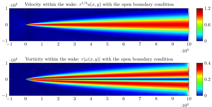
Figure 3: Velocity and vorticity profiles with the open boundary condition in an annulus of radius $R=10^{5}$. The wake is less influenced near the artificial boundary by the open boundary condition than by the no-slip boundary condition.

Figure 3 is the analogue of figure 2 but with the open artificial boundary condition. From a qualitative point of view, the wake for $u$ is almost not influenced by the open artificial boundary condition. For the vorticity $\omega$, we see some small deviations in the wake near the artificial boundary. This is expected, since the open boundary condition fixes quantities related to the derivative of $\boldsymbol{u}$ and the vorticity $\omega$ is defined trough derivatives of $\boldsymbol{u}$. Figure 5b, shows the decay of $u$ along the $x$-axis, and we see that the open boundary condition is better suited to predict the downstream behaviour. Figure 6b exhibits that the upstream behaviour is as badly predicted as with the no-slip boundary condition. Finally, the velocity and the vorticity profiles downstream (figure 7) are rather not influenced by the choice of the boundary condition. Again the upstream profiles (figure 8) are not in good agreement with the asymptotic expansion. We conclude that the open boundary condition improves the simulations downstream, but not upstream. The aim of the next subsection is to show that, when using the asymptotic expansion to define artificial boundary conditions, the results of the simulations are vastly improved in the upstream region.

3.3 Adaptive boundary conditions

Since the asymptotic expansion provides information on the behaviour of the solution at large values of $r$, it is natural to evaluate the asymptotic expansion on the artificial boundary,

$$\boldsymbol{u}_{\infty}=\left.\boldsymbol{u}_{0}\right|_{\Gamma}+\left.\boldsymbol{u}_{1}\right|_{\Gamma}\,,$$

instead of taking the value at infinity as the artificial boundary condition. The asymptotic expansion depends on the free parameter $a$, which is related to the net force acting on the body. Since the force is not known before the solution is computed, we determine $a$ by minimizing the integral $I(a)$ defined by (21) with respect to $a$. This is done numerically by using the SNOPT algorithm of COMSOL, which is a gradient method. We note that this step is not needed for the case of problem (3) since the net force (4) is known before the solution is computed. In the case $\lambda=0.8$, we find $a\approx 0.423$. As shown in figure 4a&b, the qualitative behaviour of the wake near the artificial boundary seems to be insensitive to the artificial boundary, both for the velocity and the vorticity. In figure 4c, we plot the difference between the velocity and the asymptotic expansion up to second order. This difference appears to decay like $r^{-1}$ as predicted by conjecture 1, and corresponds to the third order term $\psi_{2}=x^{-1/3}\varphi_{2}(z)$ in the asymptotic expansion (13). With the adaptive boundary condition, the decay of $u$ downstream (figure 5c) and upstream (figure 6c) is not modified by the size of the domain. We conclude that the solution can be accurately computed with this type of boundary conditions on much smaller domains than with no-slip or open boundary conditions. As can be seen, the vertical profiles downstream (figure 7) and upstream (figure 8) are so close to the second order asymptotes that the two lines essentially become indistinguishable. We take these results as a further confirmation of the correctness of the asymptotic expansion.

One of the big advantage of adaptive boundary conditions over standard boundary conditions, is that the upstream behaviour is also captured accurately. This allows to take domains much smaller without modifying the quality of the simulations, and to reduce the computational time, in spite of the disadvantage that one needs to perform multiple simulations with different values of $a$ in order to find the minimum of $I(a)$. The reason why, this techinque is not that time consuming is that the solver profits from a good initial guess in the non-linear iterations by taking the solution already computed for a nearby value of $a$.

Finally, we also analyse the solutions for smaller values of $\lambda$. As shown in movie 1, by taking $\lambda$ smaller, the parameter $a$ and the net force get also smaller, so that the amplitude of the wake decreases, and the wake becomes wider.

4 Numerical simulations with rotating boundary conditions

Recently, Hillairet & Wittwer (2013) proved the existence of solutions to (1b) for a ball of boundary conditions which contains in particular the function

$$\boldsymbol{u}^{*}=\mu\left(-y,x\right)+\lambda\left(1,0\right)\,,$$

for the case where $\mu>\sqrt{48}$ and $\lambda$ is sufficiently small. The authors prove the existence of a solution decaying uniformly like $r^{-1}$, and more precisely that the asymptotic behaviour is given by the stream function $\psi=\tilde{\mu}\log r$ where $\tilde{\mu}$ is close to $\mu$. The aim of this section is to analyse the transition from $\mu=0$, which corresponds to the case previously considered, to $\mu>\sqrt{48}$ where there is no net force. For the numerical simulations, we take $\lambda=0.8$ as before and use the parametric solver of COMSOL to vary the parameter $\mu$. Figure 9 and movie 2 show the wake for the velocity for different values of $\mu$ with no-slip boundary condition, $\boldsymbol{u}_{\infty}=\boldsymbol{0}$. We find that the more $\mu$ is increasing the more the wake is rotated, but the shape remains otherwise unchanged. Just before $\mu=\sqrt{48}$, the wake amplitude is starting to decrease and the orientation changes more rapidly, so that in a very few numerical steps of $\mu$ the wake has totally disappeared. Figure 10 shows, as a function of $\mu$, the angle $\vartheta$ between the wake and the positive real axis as well as the force acting on the body. The angle varies linearly when $\mu$ is small and apparently diverges when $\mu$ approaches $\sqrt{48}$. For $\mu>\sqrt{48}$, the wake is no more present, and the force is zero as expected. We also compute the torque $M$ on the body measured from its centre, which appears to be linearly increasing with $\mu$. The slope is approximately given by $4\pi$ which is the value analytically obtained in the case $\lambda=0$.

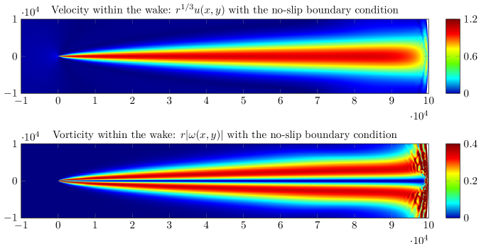
Figure 2: Velocity and vorticity profiles with the no-slip boundary condition in an annulus of radius $R=10^{5}$. The wake for $u$ has the form $u\approx x^{-1/3}\varphi_{0}^{\prime}(z)$ and the one of the vorticity $\omega\approx-x^{-1}\varphi_{0}^{\prime\prime}(z)$.

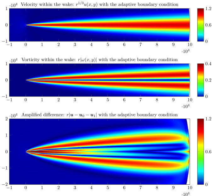
Figure 4: Velocity and vorticity profiles with the adaptive boundary condition. Difference between the numerical velocity and the asymptotic expansion: the dominant remaining term is of the form $\left|\boldsymbol{u}-\boldsymbol{u}_{0}-\boldsymbol{u}_{1}\right|\approx x^{-1}\varphi_{2}^{\prime\prime}(z)$ as expected from the computation of the third order of the asymptotic expansion.

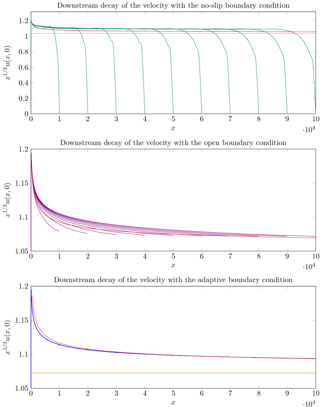
Figure 5: Downstream velocity profile within the wake with no-slip, open and adaptive boundary conditions on the outer boundary $\Gamma$ for radii $R\in\left\{1,2,\dots,10\right\}\cdot 10^{4}$.

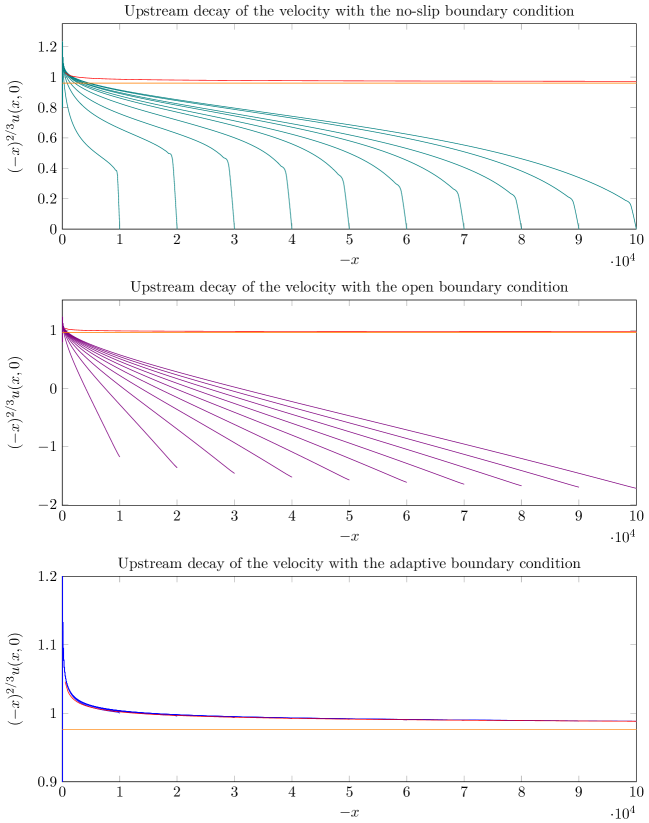
Figure 6: Upstream velocity profile with no-slip, open and adaptive boundary conditions on the outer boundary $\Gamma$ for radii $R\in\left\{1,2,\dots,10\right\}\cdot 10^{4}$.

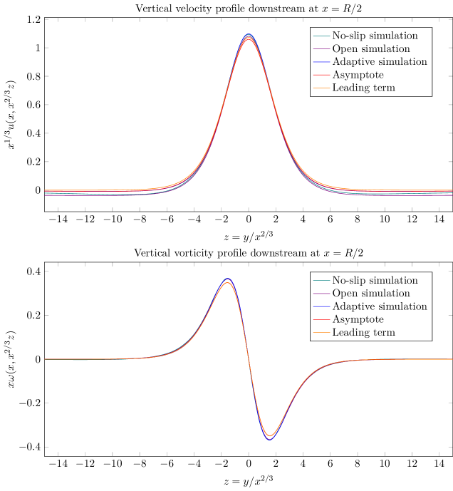
Figure 7: Velocity and vorticity profiles along the vertical line at $x=R/2$ with $R=10^{5}$ in terms of $z=y/x^{2/3}$.

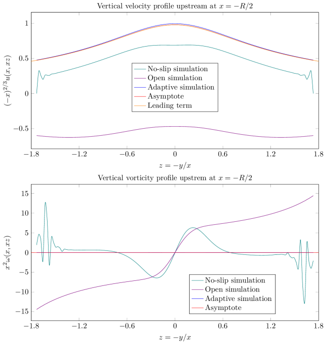
Figure 8: Velocity and vorticity profiles along the vertical line at $x=-R/2$ with $R=10^{5}$ in terms of $z=-y/x$. As expected, the vorticity in almost zero in the upstream region.

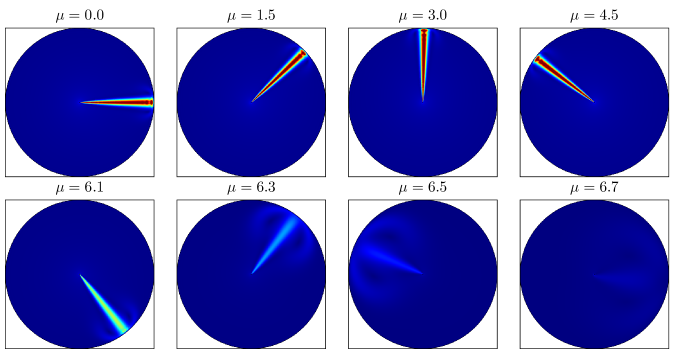
Figure 9: Magnitude of the velocity field $|\boldsymbol{x}|^{1/3}|\boldsymbol{u}|$ for different values of $\mu$ with $R=10^{5}$. As $\mu$ grows the wake starts to rotate and its amplitude decays, and for $\mu>\sqrt{48}$ the wake has totally disappeared.

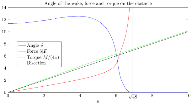
Figure 10: Magnitude of the force and torque acting on the boundary $\partial B(\boldsymbol{0},1)$ and angle $\vartheta$ of the orientation of the wake as a function of $\mu$ for $R=10^{5}$. For $\mu>\sqrt{48}$ the wake is no more present, so no angle is measured.

References

- Babenko (1973) Babenko, K. I. 1973 On stationary solutions of the problem of flow past a body by a viscous incompressible fluid. Math. USSR-Sb. 20, 1–25.
- Bichsel & Wittwer (2007) Bichsel, D. & Wittwer, P. 2007 Stationary flow past a semi-infinite flat plate: analytical and numerical evidence for a symmetry-breaking solution. Journal of Statistical Physics 127 (1), 133–170.
- Boeckle & Wittwer (2013) Boeckle, C. & Wittwer, P. 2013 Artificial boundary conditions for stationary Navier-Stokes flows past bodies in the half-plane. Computers & Fluids 82, 95–109.
- Bönisch et al. (2005) Bönisch, S., Heuveline, V. & Wittwer, P. 2005 Adaptive boundary conditions for exterior flow problems. Journal of Mathematical Fluid Mechanics 7 (1), 85–107.
- Bönisch et al. (2008) Bönisch, S., Heuveline, V. & Wittwer, P. 2008 Second order adaptive boundary conditions for exterior flow problems: Non-symmetric stationary flows in two dimensions. Journal of Mathematical Fluid Mechanics 10 (1), 45–70.
- Deuring & Galdi (2000) Deuring, P. & Galdi, G. P. 2000 On the asymptotic behavior of physically reasonable solutions to the stationary Navier-Stokes system in three-dimensional exterior domains with zero velocity at infinity. Journal of Mathematical Fluid Mechanics 2, 353–364.
- van Dyke (1975) van Dyke, M. 1975 Perturbation methods in fluid mechanics, annotated edn. Stanford, California: The Parabolic Press.
- Farwig & Sohr (1998) Farwig, R. & Sohr, H. 1998 Weighted estimates for the Oseen equations and the Navier-Stokes equations in exterior domains. Heywood, J. G. (ed.) et al., Theory of the Navier-Stokes equations. Proceedings of the third international conference on the Navier-Stokes equations: theory and numerical methods, Oberwolfach, Germany, June 5–11, 1994. Singapore: World Scientific. Ser. Adv. Math. Appl. Sci. 47, 11–30.
- Finn (1959) Finn, R. 1959 Estimates at infinity for stationary solutions of the Navier-Stokes equations. Bull. Math. Soc. Sci. Math. Phys. R. P. Roumaine (N.S.) 3 (51), 387–418.
- Finn & Smith (1967) Finn, R. & Smith, D. R. 1967 On the stationary solutions of the Navier-Stokes equations in two dimensions. Archive for Rational Mechanics and Analysis 25, 26–39.
- Galdi (1992) Galdi, G. P. 1992 On the asymptotic structure of -solutions to steady Navier-Stokes equations in exterior domains. In Mathematical problems relating to the Navier-Stokes equation (ed. G. P. Galdi), Series on advances in mathematics for applied sciences, vol. 11, pp. 81–105. World Scientific.
- Galdi (1993) Galdi, G. P. 1993 On the asymptotic properties of Leray’s solutions to the exterior steady three-dimensional Navier-Stokes equations with zero velocity at infinity. In Degenerate Diffusions (ed. Wei-Ming Ni, L. A. Peletier & J. L. Vazquez), The IMA Volumes in Mathematics and its Applications, vol. 47, pp. 95–103. Springer.
- Galdi (2004) Galdi, G. P. 2004 Stationary Navier-Stokes problem in a two-dimensional exterior domain. In Stationary partial differential equations. Vol. I, pp. 71–155. Amsterdam: North-Holland.
- Galdi (2011) Galdi, G. P. 2011 An Introduction to the Mathematical Theory of the Navier-Stokes Equations. Steady-State Problems, second edition edn. New York: Springer Verlag.
- Galdi & Sohr (1995) Galdi, G. P. & Sohr, H. 1995 On the asymptotic structure of plane steady flow of a viscous fluid in exterior domains. Archive for Rational Mechanics and Analysis 131, 101–119.
- Goldstein (1957) Goldstein, S. 1957 Lectures on Fluid Mechanics. Interscience Publishers, Ltd., London.
- Hamel (1917) Hamel, G. 1917 Spiralförmige Bewegungen zäher Flüssigkeiten. Jahresbericht der Deutschen Mathematiker-Vereinigung 25, 34–60.
- Hillairet & Wittwer (2012) Hillairet, M. & Wittwer, P. 2012 Asymptotic description of solutions of the exterior Navier-Stokes problem in a half space. Archive for Rational Mechanics and Analysis 205, 553–584.
- Hillairet & Wittwer (2013) Hillairet, M. & Wittwer, P. 2013 On the existence of solutions to the planar exterior Navier-Stokes system.
- Korolev & Šverák (2011) Korolev, A. & Šverák, V. 2011 On the large-distance asymptotics of steady state solutions of the Navier-Stokes equations in 3D exterior domains. Annales de l’Institut Henri Poincaré - Analyse non linéaire 28 (2), 303–313.
- Landau (1944) Landau, L. D. 1944 A new exact solution of the Navier-Stokes equations. Doklady Akademii Nauk SSSR 43, 286–288.
- Nazarov & Pileckas (2000) Nazarov, S. A. & Pileckas, K. 2000 On steady Stokes and Navier-Stokes problems with zero velocity at infinity in a three-dimensional exterior domain. Journal of Mathematics of Kyoto University 40, 475–492.
- Nazarov & Pileckas (1999) Nazarov, S. A. & Pileckas, K. I. 1999 Asymptotic of solutions of the Navier-Stokes equations in the exterior of a bounded body. Doklady Mathematics 60 (1), 133–135.
- Ockendon & Ockendon (1995) Ockendon, H. & Ockendon, J. R. 1995 Viscous Flow. Cambridge University Press.
- Pileckas & Russo (2012) Pileckas, K. & Russo, R. 2012 On the existence of vanishing at infinity symmetric solutions to the plane stationary exterior Navier-Stokes problem. Mathematische Annalen 352 (3), 643–658.
- Russo (2008) Russo, A. 2008 On the steady-state Navier-Stokes equations in two dimensional domains. PhD thesis, Università di Napoli "Federico II".
- Sazonov (1999) Sazonov, L. I. 1999 Asymptotic behavior of the solution to the two-dimensional stationary problem of flow past a body far from it. Mathematical Notes 65 (2), 202–207.
- Šverák (2011) Šverák, V. 2011 On Landau’s solutions of the Navier-Stokes equations. Journal of Mathematical Sciences 179 (1), 208–228, translated from Problems in Mathematical Analysis 61, October 2011, pp. 175-190.
- Yamazaki (2009) Yamazaki, M. 2009 The stationary Navier-Stokes equation on the whole plane with external force with antisymmetry. Annali dell’Universita di Ferrara 55, 407–423.
- Yudovich (2003) Yudovich, V. I. 2003 Eleven great problems of mathematical hydrodynamics. Moscow Mathematical Journal 3 (2), 711–737.