Explosive synchronization in weighted complex networks

Abstract

The emergence of dynamical abrupt transitions in the macroscopic state of a system is currently a subject of the utmost interest. Given a set of phase oscillators networking with a generic wiring of connections and displaying a generic frequency distribution, we show how combining dynamical local information on frequency mismatches and global information on the graph topology suggests a judicious and yet practical weighting procedure which is able to induce and enhance explosive, irreversible, transitions to synchronization. We report extensive numerical and analytical evidence of the validity and scalability of such a procedure for different initial frequency distributions, for both homogeneous and heterogeneous networks, as well as for both linear and non linear weighting functions. We furthermore report on the possibility of parametrically controlling the width and extent of the hysteretic region of coexistence of the unsynchronized and synchronized states.

PACS: 89.75.Hc, 89.75.Kd, 89.75.Da, 64.60.an,05.45.Xt.

I Introduction

One of the most significant challenges of present-day research is bringing to light the processes underlying the spontaneous organization of networked dynamical units. When a network passes from one to another collective phase under the action of a control parameter, the nature of the associated phase transition is disclosed by the behavior of the order parameter at criticality: continuous for second-order transitions and discontinuous for first-order ones. In complex networks’ theory Boccaletti2006 ; Dorogovtsev2008 such phase transitions have been observed in the way a graph collectively organizes its architecture through percolation Karsai2007 ; Achlioptas09 ; various2 , and its dynamical state through synchronization Boccaletti2002 ; Arenas2008 .

Abrupt transitions to synchronized states of networked phase oscillators were initially reported in a Kuramoto model kuramoto for a particular realization of a uniform frequency distribution (evenly spaced frequencies) and an all-to-all network topology pazo . Later on, the same finding was also described for both periodic jesus1 and chaotic leyva12 phase oscillators in the yet particular condition of a heterogeneous degree-distribution with positive correlations between the node degree and the corresponding oscillator’s natural frequency. Recently, Ref. Zhang13 introduced a more general framework where explosive synchronization (ES) is obtained in weighted networks, where weights are selected to be proportional to the absolute value of the frequency of the oscillators in a way that produces positive correlations between the node strength and the frequency of the oscillator.

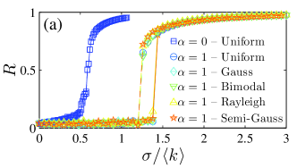
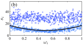
Figure 1: (Color online). (a) Synchronization transitions for N=500 ER networks, $\langle k\rangle$=30, for un-weighted case ($\alpha=0$) (blue squares), and linearly weighted cases ($\alpha=1$) with several frequency distributions within the range $[0,1]$: uniform, Gaussian, Gaussian-derived, Rayleigh and semi-Gaussian. Solid and dashed lines refer to the forward and backward simulations, respectively. (b) Node strengths $s_{i}$ (see text for definition) vs. natural frequencies $\omega_{i}$, for the un-weighted (dark blue squares) and weighted (light bue circles) networks reported in (a). Solid line is proportional to the analytical prediction $(\omega-\frac{a}{2})^{2}+\frac{1}{4a}$ in the thermodynamical limit of our model, with $a=1$ the width of the uniform frequency distribution (see text for more details).

The weighting procedure proposed in Ref. Zhang13 inherently asymmetrizes each link of the network, favoring the interaction directions from higher to lower frequencies. In this work, we propose an alternative general framework for ES in complex networks, based on a weighting procedure which instead keeps the symmetric nature of the links. The method is inspired by our recent study of Ref. leyvanat , where it is shown that ES can be obtained for any given frequency distribution, provided the connection network is constructed following a rule of frequency disassortativity, that is, that the synchronization clustering formation is prevented avoiding close frequencies to couple, in a network generation scheme ruled by dynamical properties, as the Achlioptas rule Achlioptas09 works for the structural case in explosive percolation.

We here deal with the more general case of a network with given frequency distribution and architecture, and we show that a weighting procedure on the existing links, that combines information on the frequency mismatch of the two end oscillators of a link with that of the link betweenness, has the effect of inducing or enhancing ES phenomena for both homogeneous and heterogeneous graph topologies, as well as any symmetric or asymmetric frequency distribution. In addition, we show the general scaling properties of the obtained transition, and provide analytical arguments in support of our claims.

II Model and numerical results

Without lack of generality, our reference is a network $\cal{G}$ of $N$ Kuramoto kuramoto phase oscillators, described by:

$$\frac{d\theta_{i}}{dt}=\omega_{i}+\frac{\sigma}{\left<k\right>}\sum_{i=1}^{N}\Omega_{ij}^{\alpha}\sin(\theta_{j}-\theta_{i}),$$ (1)

where $\theta_{i}$ is the phase of the $i^{th}$ oscillator ($i=1,...,N$), $\omega_{i}$ is its associated natural frequency drawn from a frequency distribution $g(\omega)$, $\sigma$ is the coupling strength, $\langle k\rangle$ is the graph average connectivity ($\langle k\rangle\equiv\frac{2L}{N}$, with $L$ being the total number of links), and

$$\Omega_{ij}^{\alpha}=a_{ij}|\omega_{i}-\omega_{j}|^{\alpha},$$ (2)

is the weighted link for nodes $i,j$, being $a_{ij}$ the elements of the adjacency matrix that uniquely defines $\cal{G}$ and $\alpha$ a constant parameter which eventually modulates the weight. The strength of the $i^{th}$ node (the sum of all its links weights) is then $s_{i}=\sum_{j}\Omega_{ij}^{\alpha}$. The classical order parameter for system (1) is $r(t)=\frac{1}{N}|\sum_{j=1}^{N}e^{i\theta_{j}(t)}|$, and the level of synchronization can be monitored by looking at the value of $R=\langle r(t)\rangle_{T}$, with $\langle...\rangle_{T}$ denoting a time average over a conveniently large time span $T$.

As the coupling strength $\sigma$ increases, system (1) undergoes a phase transition at a critical value $\sigma_{c}$ from the unsynchronized ($R\sim 1/\sqrt{N}$) to the synchronous ($R=1$) state, where all oscillators ultimately acquire the same frequency. In the following, we will describe the nature of such a transition as a function of the re-scaled order parameter $\sigma/\langle k\rangle$. As for the stipulations followed in our simulations, the state of the network is monitored by gradually increasing $\sigma$ in steps $\delta\sigma=0.0005$, starting at $\sigma=0$. Whenever a step $\delta\sigma$ is made, a long transient (200 time units) is discarded before the data are recorded and processed. Moreover, as we are focusing on abrupt, irreversible transitions (and thus on expected associated hysteretic phenomena), we perform the simulations also in the reverse way, i.e. starting from a given value $\sigma_{\max}$ (where $R=1$), and gradually decreasing the coupling by $\delta\sigma$ at each step. In what follows, the two sets of numerical trials are termed as forward and backward, respectively.

II.1 Homogeneous networks

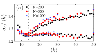
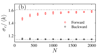
Figure 2: (Color online) Critical scaled coupling $\sigma_{c}/\langle k\rangle$ at the onset of synchronization/desynchronization using a linear weighting procedure $\Omega_{ij}$ ($\alpha=1$) as a function of (a) $\langle k\rangle$ for several ER network sizes $N$, and of (b) $N$ in all-to-all coupled networks. In (a) vertical dashed line marks the passage from a smooth to an explosive phase transition. Both in (a) and (b) upper and lower branches correspond to forward and backward simulations, respectively. Each dot accounts for an average of at least 20 independent runs of uniform frequency distributions. Horizontal dashed lines in (b) are close to the analytical values defining the range of the hysteresis in the thermodynamical limit for the Kuramoto model (see explanation in the text). Frequencies are uniformly distributed in the range $[0,1]$.

We first report our results on the case of homogeneous graph topologies. For this purpose, we consider Erdös-Rényi (ER) random networks erdos of size $N$, and we describe how an explosive transition is induced, for sufficiently large values of $\langle k\rangle$ and irrespectively on the specific frequency distribution $g(\omega)$. Figure 1(a) reports the results for $N=500$ and several frequency distributions $g(\omega)$ within the range $[0,1]$. For the simplest case of uniform frequency distribution $g(\omega)$=1, while the un-weighted network ($\alpha=0$ in Eq. 2) displays a smooth, second-order like transition to synchronization [dark blue curve in Fig. 1(a)], the effect of a linear weighting ($\alpha=1$) is that of inducing a sharp transition in the system, with an associated hysteresis in the forward (solid line) and backward (dashed line) simulations. This drastic change in the nature of the transition is independent of the frequency distribution $g(\omega)$, as long as they are defined in the same frequency range $[0,1]$ as shown in Fig. 1(a). The results are identical for symmetric distributions (homogeneous, Gaussian, a bimodal distribution derived from a Gaussian) and for asymmetric frequency distributions (Rayleigh, a Gaussian centered at $0$ but just using the positive half). See details of the used frequency distributions in distributions .

Figure 1(b) accounts for the existence of a parabolic relationship between the strengths and the natural frequencies of the oscillators associated with the passage from a smooth to an explosive phase transition. This relationship has been obtained analytically (see Eq.(7)) in the thermodynamical limit of the Kuramoto model and perfectly fits the numerical results shown as a solid line in Fig. 1(b). It has to be remarked that, while in Ref. jesus1 degree-frequency correlation features were imposed to determine explosiveness in the transition to synchronization, here the effect of the weighting is to let these topological/dynamical correlation features spontaneously emerge, with the result of shaping a bipartite-like network where low and high frequency oscillators are the ones with maximal overall strength.

Further information about the nature and scaling properties of the transition induced by the linear weighting procedure is gained from Fig. 2, where it is shown the dependence of the scaled critical coupling $\sigma_{c}/\langle k\rangle$ on the average connectivity $\langle k\rangle$ and on the network size $N$. Precisely, Fig. 2(a) shows that, independently on $N$, a dynamical bifurcation exists at ${\langle k\rangle}\sim 17$, corresponding to the passage from a second- to a first-order like phase transition. For the latter regime, the two branches expanding from $\langle k\rangle\gtrsim 17$ are associated to the hysteresis in the forward and backward simulations. The relative independence on $N$ can be explained considering that an important condition for ES to occur is that each node neighborhood must represent a statistically significant sample of the network frequencies up to give a close enough approximation to the global mean frequency, and therefore the synchronization frequency. To reach this target, the required sampling size $n$ for a given population size $N$ is usually calculated with the following formula Cochran77

$$n=\frac{N}{1+C^{2}(N-1)},$$

where $C:=2e/z_{\alpha/2}$, being $e$ the error allowed, $1-\alpha$ the confidence level, and $z_{\alpha/2}$ the upper $\alpha/2$ percentage point of the standard normal distribution. Aside from the technical details, the important feature in the expression is that the sampling size converges to a finite value, even for an infinite population. This is exactly what Fig. 2(a) shows. Once the mean degree is large enough, each node has a neighborhood assuring that its neighbor frequency average is statistically accurate. Precisely, Fig. 2(a) suggests that $C\approx 0.24$, indicating that, for mean degrees greater than $\sim$17, each node has a sufficiently large neighborhood independently of the population size $N$. Figure 2(b) shows how the scaled critical couplings defining the hysteresis of the ES transition converge to constant values for the Kuramoto model (all to all coupling) when $N$ increases which are quite close to those obtained in the thermodynamical limit of the Kuramoto model discussed in the analytical section.

Furthermore, the weighting procedure inducing ES is quite general, as a large family of detuning dependent functions can be used. As an example, Fig. 3 describes the case of nonlinear weighting procedures, that is, $\alpha\neq 1$ in Eq. (2). There, we set again $N=500$ and $\langle k\rangle=30$ and consider both ER graphs (Fig. 3(a)), and a regular random network (Fig. 3(b)), i.e. a network where each node has exactly the same number of connections ($k_{i}=\langle k\rangle=30$) with the rest of the graph. This latter case has been obtained by a simple configuration model configuration , imposing a $\delta$-Dirac degree distribution. The results in Fig. 3 show that the generic non-linear function of the frequency mismatch given by Eq. (2) is able to induce ES in both topologies, and that the effect of a super-linear ($\alpha>1$) weighting (a sub-linear ($\alpha<1$) weighting) is that of enhancing (reducing) the width of the hysteretic region.

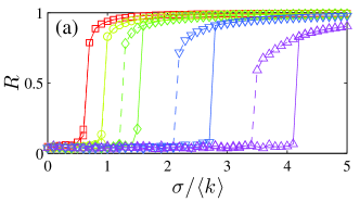
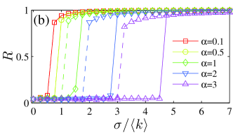
Figure 3: (Color online). Synchronization transitions for ER networks, $N=500$, uniformly distributed frequencies in the $[0,1]$ range, and nonlinear weighting functions $\Omega_{ij}^{\alpha}$. Both plots consider several $\alpha$ values, from sub-linear to super-linear weighting (see legend in panel b). (a) ER networks, $\langle k\rangle=30$, (b) regular random networks, $k=30$. In all cases, forward and backward simulations correspond respectively to solid and dashed lines.

II.2 Heterogeneous networks

So far, we have considered only homogeneous degree distributions. In order to properly describe the passage from a homogeneous to a heterogeneous degree distribution, we rely on the procedure introduced in Ref. Gomez-Gardenes06 . Such a technique, indeed, allows constructing graphs with the same average connectivity $\langle k\rangle$, and grants one the option of continuously interpolating from ER to scale-free (SF) networks Albert1999 , by tuning a single parameter $0\leq p\leq 1$. With this method, networks are grown from an initial small clique, by sequentially adding nodes, up to the desired graph size. Each newly added node has a probability $p$ of forming random connections with already existing vertices, and a probability $1-p$ of following a preferential attachment rule Albert1999 for the selection of its connections. As a result, the limit $p=1$ induces an ER configuration, whereas the limit $p=0$ corresponds to a SF network with degree distribution $P(k)\sim k^{-3}$.

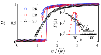
Figure 4: (Color online) Explosive synchronization vs. degree heterogeneity. Synchronization transitions as a function of the coupling strength for linearly weighted networks ($\alpha=1$) with the same average connectivity $\langle k\rangle=30$, but a different second moment of the degree distribution: a regular random (RR) network with homogeneous degree $\sigma_{k}=0$ (blue circles), an ER network (red squares) and a SF (black triangles). In all cases, forward and backward simulations correspond respectively to solid and dashed lines. Inset: log-log plot of the three corresponding degree distributions.

Let us set $N=1000$ and $\langle k\rangle=30$ and, after the network construction, let us randomly distribute the oscillators’ frequencies in the interval $[0,1]$ and use again a linear weighting function $\Omega_{ij}=a_{ij}|\omega_{i}-\omega_{j}|$. The comparative results are reported in Fig. 4, from which it is easy to see that heterogeneity in the degree distribution actually opposes the onset of explosive synchronization. A similar qualitative scenario (not shown) is obtained also for different frequency distributions, network’s sizes, and (super-linear or sub-linear) weighting functions, allowing one to conclude that heterogeneous degree-distributions require a different weighting approach, where the information on frequency mismatch has to be properly combined with local or global information on the network topology.

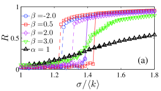
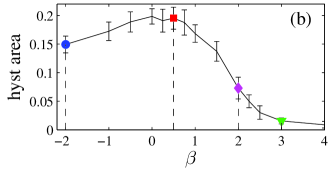
Figure 5: (Color online). (a) Synchronization transitions for SF networks using different schemes of coupling weighting. In black triangles, the link between nodes $i$ and $j$ is weighted using $\Omega_{ij}^{\alpha}$ with $\alpha=1$ (as in Fig. 4), while the rest of cases refer to the weighting function $\widetilde{\Omega}_{ij}$ of Eq.(3), with the values of the $\beta$ parameter given in the legend. In all cases, forward and backward simulations correspond respectively to continuous and dashed lines. (b) Area of the hysteretic region vs. $\beta$. Each point is an average of 10 different simulations, each one starting from a different realization of the frequency distributions. In all cases, $\langle k\rangle=30$, $N=1000$ and natural frequencies uniformly distributed in the interval $[0,1]$.

The problem closely resembles what was called, in past years, the paradox of heterogeneity nishi where increasing the heterogeneity in the connectivity distribution of a unweighted network led to an overall deterioration of synchrony, despite the associated reduction of the network’s shortest path. That paradox was lately solved by proving optimal synchronization conditions when proper weighting procedures are implemented on the graph’s links accounting for either local motter or global bocca information on the specific network topology. Therefore, in analogy with what reported in Ref. bocca , we consider a new weighting function

$$\widetilde{\Omega}_{ij}=a_{ij}|\omega_{i}-\omega_{j}|\displaystyle\frac{\ell_{ij}^{\beta}}{\sum_{j\in{\cal{N}}_{i}}\ell_{ij}^{\beta}},$$ (3)

with $\beta$ being a parameter and $\ell_{ij}$ the edge betweenness associated to the link $a_{ij}$ newman , defined as the number of shortest paths between pairs of nodes in the network that run through that edge.

The results are reported in Fig. 5(a). While the case $\beta=0$ (black triangles, already shown in Fig. 4) corresponds to a smooth transition, the effect for $\beta\neq 0$ in Eq.(3) is highly nontrivial. Precisely, moderate (positive or negative) values of $\beta$ establish in system (1) an abrupt transition to synchronization. However, increasing $\beta$ beyond a critical value leads system (1) to display again a smooth and reversible character of the transition.

On its turn, Fig. 5(b) reports the hysteresis’ area (the area of the plane ($R,\sigma/\langle k\rangle$) covered by the hysteretic region) as a function of $\beta$, obtained by an ensemble average over 10 different forward and backward simulations of system (1) together with the weighting function (3), each one starting from a different realization of the uniform frequency distribution. The plot reveals the existence of an optimal condition at around $\beta=0.5$ where the width of the hysteresis is maximized. Therefore, $\beta$ can be seen as an operational parameter through which one can control and regulate the width and extent in $\sigma$ of the hysteresis associated with the irreversible nature of ES. The latter can be of interest for controlling the range of coupling strength for which system (1) can be used to originate magnetic-like states of synchronization, i.e. situations in which an originally unsynchronized configuration, once entrained to a given phase by an external pacemaker acting for a limited time lapse, is able to permanently stay in a synchronized configuration leyvanat .

III Analytical results

In order to study the onset and nature of the explosive transition, we must analytically examine the behavior of the system in the thermodynamic limit. Let us consider the paradigmatic case in which $N$ oscillators form a fully connected graph, as the original Kuramoto model, but with weights $\Omega_{ij}=|\omega_{i}-\omega_{j}|$. Then, the dynamical equations are

$$\dot{\theta}_{i}=\omega_{i}+\frac{\sigma}{N}\sum_{j=1}^{N}\Omega_{ij}\sin(\theta_{j}-\theta_{i}),$$

for $i=1,\ldots N$.

By considering the following definitions,

$$\frac{1}{N}\sum_{j=1}^{N}\Omega_{ij}\sin\theta_{j} := A_{i}\sin\phi_{i},$$

$$\frac{1}{N}\sum_{j=1}^{N}\Omega_{ij}\cos\theta_{j} := A_{i}\cos\phi_{i}.$$

the dynamical equations are usually expressed Strogatz00 in terms of trigonometric functions as

$$\dot{\theta}_{i}=\omega_{i}+\sigma A_{i}\sin(\phi_{i}-\theta_{i}).$$

While these transformations are the same as those used in the original Kuramoto model, now there is an explicit dependence on $i$ in the quantities $A_{i}$ and $\phi_{i}$. In order to continue our analysis, we will then assume some mild approximations.

In the co-rotating frame, the phases must verify $\omega_{i}=\sigma A_{i}\sin(\theta_{i}-\phi_{i})$ to have a static solution (i.e., $\dot{\theta}_{i}=0$), which in the thermodynamic limit reads

$$\omega=\sigma A_{\omega}\sin(\theta_{\omega}-\phi_{\omega}).$$ (4)

The definition of $A_{\omega}$ and $\phi_{\omega}$ implies that

$$F(\omega):=A_{\omega}\sin\phi_{\omega}=\int g(x)|w-x|\sin\theta(x)\,dx,$$

whose second derivative verifies

$$F^{\prime\prime}(\omega)=\int g(x)2\delta(w-x)\sin\theta(x)\,dx=2g(\omega)\sin\theta(\omega),$$

using the distributional derivative of the signum function. Likewise, if we consider

$$G(\omega):=A_{\omega}\cos\phi_{\omega}=\int g(x)|w-x|\cos\theta(x)\,dx,$$

its second derivative verifies

$$G^{\prime\prime}(\omega)=2g(\omega)\cos\theta(\omega).$$

Then, Eq.  (4) takes the form

$$\frac{2}{\sigma}g(\omega)\omega=F^{\prime\prime}(\omega)G(\omega)-F(\omega)G^{\prime\prime}(\omega).$$ (5)

Let us work out $F(\omega)$ and $G(\omega)$. When all oscillators are close to synchronization, we can assume that $\cos\theta(x)\approx R$, thus

$$G(\omega)\approx R\int g(x)|w-x|\,dx=Rs(\omega),$$

where $s(\omega)$ is just the strength of a node with intrinsic frequency $\omega$. Therefore, Eq. (5) can be approximated by

$$\frac{2}{R\sigma}g(\omega)\omega=F^{\prime\prime}(\omega)s(\omega)-F(\omega)s^{\prime\prime}(\omega),$$ (6)

which is a second order ODE whose integration yields $F(\omega)$. Notice that when $s(\omega)$ is a rather involved function, Eq. (6) is already an approximation, and we can just consider a polynomial expansion in $\omega$ to obtain an analytical expression of $F(\omega)$.

For instance, given a uniform distribution $g(\omega)$ in the interval $[-a/2,+a/2]$, the resulting strength is a second order polynomial,

$$s(\omega)=a\left[\left(\frac{\omega}{a}\right)^{2}+\frac{1}{4}\right],$$ (7)

which perfectly fits our numerical simulations (see Fig. 1(b)), even though it has been deduced for a complete graph. Then, the integration of Eq. (6) results in

$$F(\omega)=a\frac{\left[1+4\left(\frac{\omega}{a}\right)^{2}\right]\arctan\left(\frac{2w}{a}\right)-(2+\pi)\frac{w}{a}}{(4+\pi)\sigma R},$$

using the initial condition $F(0)=0$, since $g(\omega)$ is a symmetric function (thus $F(\omega)$ is an odd function), and the consistency equation

$$F(\omega)=\int g(x)|\omega-x|\sin\theta(x)\,dx=\int\frac{|\omega-x|}{2}F^{\prime\prime}(x)\,dx.$$

Therefore, since $F^{\prime\prime}(\omega)=2g(\omega)\sin\theta(\omega)$, we find that

$$\sin\theta(\omega)=\frac{1}{\sigma R}\,H\left(\frac{2\omega}{a}\right),$$

where

$$H(z):=\frac{4}{4+\pi}\left[\frac{z}{1+z^{2}}+\arctan(z)\right].$$

To determine how the order parameter $R$ depends on the coupling constant $\sigma$, we use that

$$R=\int g(x)\cos\theta(x)\,dx=\int g(x)\sqrt{1-\sin^{2}\theta(x)}\,dx,$$ (8)

which is an implicit equation in $R$. When $\sigma R\geq\frac{2+\pi}{4+\pi}\approx 0.72$, $\sin\theta(x)\leq 1$ for all $x$, which means that all oscillators are frequency locked and, then,

$$R=\int_{-\frac{a}{2}}^{\frac{a}{2}}g(x)\sqrt{1-\left[\frac{1}{\sigma R}H\left(\frac{2x}{a}\right)\right]^{2}}\,dx.$$

When $\sigma R\leq\frac{2+\pi}{4+\pi}$, only those oscillators with frequency in the interval $[-\omega^{*},\omega^{*}]$ are locked, being

$$\omega^{*}:=\frac{a}{2}H^{-1}(\sigma R),$$

thus

$$R=\int_{-\frac{a}{2}H^{-1}(\sigma R)}^{\frac{a}{2}H^{-1}(\sigma R)}g(x)\sqrt{1-\left[\frac{1}{\sigma R}H\left(\frac{2x}{a}\right)\right]^{2}}\,dx.$$

Hence, if we define

$$\ell(\mu):=\left\{\begin{array}[]{ll}1&\text{ if }\mu\geq\frac{2+\pi}{4+\pi}\\ H^{-1}(\mu)&\text{ if }0\leq\mu<\frac{2+\pi}{4+\pi}\\ \end{array}\right.$$

and

$$I(\mu):=\int_{0}^{\ell(\mu)}\sqrt{1-\left[\frac{1}{\mu}H(z)\right]^{2}}\,dz,$$

Eq. (8) takes the form

$$\frac{\mu}{\sigma}=I(\mu),$$ (9)

being $\mu=\sigma R$. Therefore, given a coupling constant $\sigma$, the value of $R$ is computed by solving this implicit equation in $\mu$. Notice that, geometrically, the solutions are the points where the straight line passing through the origin with slope $1/\sigma$ intersects $I(\mu)$.

The main feature characterizing $I(\mu)$ is its inflection point at $\frac{2+\pi}{4+\pi}$, at which the curve changes from being concave up to concave down (see Fig. (6)). This implies that, depending on $\sigma$, there are three qualitatively different type of solutions. When $\sigma$ is small, we have the trivial solution $R=0$ since the straight line and $I(\mu)$ only intersect at $\mu=0$. This situation changes when $\sigma$ is such that the slope of the straight line is tangent to $I(\mu)$ (i.e., when $\sigma=1.03$, corresponding to the red dashed line in Fig.6(a)). When $\sigma$ is greater than this value, we enter into the region where the hysteresis takes place since, now, there are three values of $R$, two of them are stable solutions ($R=0$ and $R\approx 1$) and the third one is a unstable solution (see Fig. 6(b)). The solution $R\approx 1$ appears therefore abruptly, due to the existence of the inflection point. This behavior changes when the slope of the straight line is tangent to $I(0)$ (i.e., when $\sigma=1.43$, corresponding to the blue dashed line in Fig.6(a)), which is the point where the stable solution $R=0$ collapses with the unstable one, becoming unstable (see Fig.6(b)). Notice that the numerical values obtained for the Kuramoto model for large $N$ in Fig. 2(b) are quite close to those predicted by the theory.

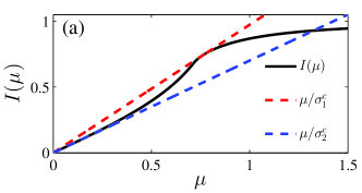
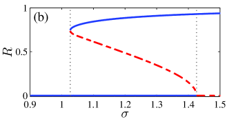
Figure 6: (Color online). (a) $I$ as a function of $\mu=\sigma R$ (solid curve) as given by Eq. (9). The dashed lines are those straight lines whose intersection with $I$ marks the backward ($\sigma_{1}^{c}$) and forward ($\sigma_{2}^{c}$) critical points of ES for an all to all connected network and for a uniform frequency distribution. (b) The corresponding synchronization order parameter $R$ as a function of the coupling strength. Solid (dashed) curves correspond to the stable (unstable) solution. Dotted vertical lines mark the region of hysteresis defined by $\sigma_{1}^{c}$ and $\sigma_{2}^{c}$ in (a).

IV Conclusions

In conclusion, we have introduced a weighting procedure based on the link frequency mismatch and on the link betweenness to induce an explosive transition to synchronization in a generic complex network of phase oscillators and for a generic distribution of the frequencies. As a consequence of this procedure, topological/dynamical correlation features spontaneously emerge, with the result of shaping a bipartite-like network where frequency disassortativity prevails.

In this scenario, the passage from a smooth to an abrupt transition has found to be fully rescalable, and critically depends only on the average connectivity, and not on the network size.

In addition, we analytically proved that our weighting procedure yields a first-order like transition whose hysteresis extent is calculated. Moreover, the theoretical framework allows for a geometrical interpretation of the explosive transition in which the weighting imposes a multi-valued Kuramoto phase order parameter, in contrast with the classical model.

The present results could provide significant insights into the study of real complex networks such as power grids which can be modeled as networks of phase oscillators whose coupling may depend on the dynamics of the nodes motter2 .

References

- (1) S. Boccaletti, V. Latora, Y. Moreno, M. Chavez and D.U. Hwang, Phys. Rep. 424, 175 (2006).
- (2) S. N. Dorogovtsev, A.V. Goltsev, and J. F. F. Mendes, Rev. Mod. Phys. 80, 1275 (2008).
- (3) R. Cohen, D. ben-Avraham and S. Havlin, Phys. Rev. E 66, 036113 (2002); M. Karsai, J-Ch. Anglès d’Auriac and F. Iglói, Phys. Rev. E 76, 041107 (2007); G. Li, L.A. Braunstein, S.V. Buldyrev, S. Havlin and H.E. Stanley, Phys. Rev. E 75, 045103 (2007).
- (4) D. Achlioptas, R.M. D’Souza and J. Spencer, Science 323, 1453 (2009).
- (5) Y.S. Cho, J.S. Kim, J. Park, B. Kahng and D. Kim, Phys. Rev. Lett. 103, 135702 (2009); F. Radicchi and S. Fortunato, Phys. Rev. Lett. 103, 168701 (2009); P. Grassberger, C. Christensen, G. Bizhani, S.-W. Son and M. Paczuski, Phys. Rev. Lett. 106, 225701 (2011).
- (6) S. Boccaletti, J. Kurths, G. Osipov, D.L. Valladares and C.S. Zhou, Phys. Rep. 366, 1 (2002).
- (7) A. Arenas, A. Díaz-Guilera, J. Kurths, Y. Moreno and C. S. Zhou, Phys. Rep. 469, 93 (2008).
- (8) Y. Kuramoto, Chemical oscillations, waves and turbulence (Springer, 1984).
- (9) D. Pazó, Phys. Rev. E 72, 046211 (2005).
- (10) J. Gómez-Gardeñes, S. Gómez, A. Arenas and Y. Moreno, Phys. Rev. Lett. 106, 128701 (2011).
- (11) I. Leyva, R. Sevilla-Escoboza, J. M. Buldú, I. Sendiña-Nadal, J. Gómez-Gardeñes, A. Arenas, Y. Moreno, S. Gómez, R. Jaimes-Reátegui, S. Boccaletti. Phys. Rev. Lett. 108, 168702 (2012).
- (12) X. Zhang, X. Hu, J. Kurths and Z. Liu. Phys. Rev. E 88, 0108012(R) (2013).
- (13) I. Leyva, A. Navas, I. Sendiña-Nadal, J. A. Almendral, J. M. Buldú, M. Zanin, D. Papo and S. Boccaletti, Nature Sci. Rep. 3, 1281 (2013).
- (14) P. Erdös and A. Rényi, Publ. Math. Debrecen 6, 290 (1959).
- (15) The details of the used distributions are: Gaussian with =0.23, a bimodal distribution derived from a Gaussian ( if , and , Rayleigh distribution with =10 and normalized to the [0,1] range, distribution derived from a Gaussian centered at but just using the positive half with , named as semi-Gaussian in Fig. 1.
- (16) G. W. Cochran. Sampling Techniques, pp 74-76. Ed. John Willey & Sons. New York 1977.
- (17) E.A. Bender and E.R. Canfield, J. Combin. Theory Ser. A 24, 296 (1978).
- (18) J. Gómez-Gardeñes and Y. Moreno, Phys. Rev. E 73, 056124 (2006).
- (19) A.-L. Barabási and R. Albert, Science 286, 509 (1999).
- (20) T. Nishikawa, A.E. Motter, Y.-C. Lai and F.C. Hoppensteadt, Phys. Rev. Lett. 91, 014101 (2003).
- (21) A.E. Motter, C.S. Zhou and J. Kurths, Europhys. Lett. 69, 334 (2005); Phys. Rev. E 71, 016116 (2005).
- (22) M. Chavez, D.-U. Hwang, A. Amann, H.G.E. Hentschel and S. Boccaletti, Phys. Rev. Lett. 94, 218701 (2005).
- (23) M.E.J. Newmann and M. Girvan, Phys. Rev. E 69, 026113 (2004).
- (24) S. H. Strogatz, Physica D 143, 1 (2000).
- (25) A.E. Motter, S.A. Myers, M. Anghel, T. Nishikawa, Nat. Physics 9, 191 (2013).