Re-summation of fluctuations near ferromagnetic quantum critical points

Abstract

We present a detailed analysis of the non-analytic structure of the free energy for the itinerant ferromagnet near the quantum critical point in two and three dimensions. We analyze a model of electrons with an isotropic dispersion interacting through a contact repulsion. A fermionic version of the quantum order-by-disorder mechanism allows us to calculate the free energy as a functional of the dispersion in the presence of homogeneous and spiralling magnetic order. We re-sum the leading divergent contributions, to derive an algebraic expression for the non-analytic contribution to free energy from quantum fluctuations. Using a recursion which relates sub-leading divergences to the leading term, we calculate the full $T=0$ contribution in $d=3$. We propose an interpolating functional form, which allows us to track phase transition lines at temperatures far below the tricritical point and down to $T=0$. In $d=2$, quantum fluctuations are stronger and non-analyticities more severe. Using a similar re-summation approach, we find that despite the different non-analytic structures, the phase diagrams in two and three dimensions are remarkably similar, exhibiting an incommensurate spiral phase near to the avoided quantum critical point.

I Introduction

Quantum fluctuations can have a dramatic effect on the phase behavior of the itinerant ferromagnet in the vicinity of the $T=0$ quantum critical point. In a pioneering paper,Hertz (1976) Hertz suggested that fluctuations can lead to new scaling in the physical quantities above the quantum critical point, which he termed “quantum critical scaling”. The theory of ferromagnetic quantum criticality was further developed by MoriyaMoriya (1985) and Millis.Millis (1993) More recently, several authors Belitz et al. (1997, 1999); Chubukov et al. (2004); Betouras et al. (2005); Rech et al. (2006); Efremov et al. (2008); Maslov and Chubukov (2009) noted that the coupling of soft electronic particle-hole modes to the magnetic order parameter generates non-analytic terms in the free energy that render the magnetic transitions first-order at low temperatures. Such fluctuation-induced first-order behavior is expected for ferromagnets in the Ising, XY, and Heisenberg universality classes in dimensions $1<d\leq 3$, regardless of whether the moments are supplied by the conduction electrons or by electrons in another band.Kirkpatrick and Belitz (2012) Such first-order behaviour is also stable against weak disorder.Belitz et al. (1997, 2001) This explains why discontinuous ferromagnetic transitions are seen in various materials, including MnSi (Ref. Pfleiderer et al., 2001), $\textrm{Sr}_{1-x}\textrm{Ca}_{x}\textrm{Ru}\textrm{O}_{3}$ (Ref. Uemura et al., 2007), CoO₂ (Ref. Otero-Leal et al., 2008), $\textrm{U}\textrm{Ge}_{2}$ (Ref. Taufour et al., 2010), and URhGe (Ref. Yelland et al., 2011).

It has been arguedChubukov et al. (2004) that fluctuation-driven first-order transitions are indicative of the appearance of precursor, incommensurate magnetic states. Recently, this possibility has been explored in $d=3$ within a fermionic version of the quantum order-by-disorder mechanism.Conduit et al. (2009); Karahasanovic et al. (2012); Krüger et al. (2012) The central idea is to self-consistently calculate fluctuations around magnetically ordered states. This approach not only reproduces the non-analytic free energy of the homogeneous ferromagnet within a much simpler calculation, but also predicts the formation of an incommensurate spiral state, pre-empting the first-order transition into the ferromagnet. Spiral formation may be driven in mean-field by e.g. a feature in the density of states Berridge et al. (2009, 2010); Igoshev et al. (2012); Katanin et al. (2011); Igoshev2 et al. (2011) or a breaking of inversion symmetry by the crystal structure, resulting in a Dzyaloshinski-Moriya interaction. Moriya (1960); Dzyaloshinsky (1958); Bak et al. (1980) Our mechanism for spiral formation does not require either of these complications, and is driven by quantum fluctuations of intinerant electrons with a simple, isotropic dispersion.

The quantum order-by-disorder phenomenon has much in common with the Coleman-Weinberg mechanism of mass generation in high energy physicsColeman and Weinberg (1973) and with the Casimir effect.Casimir and Polder (1948) It is familiar in the context of condensed matter physics.Villain, J. et al. (1980); Chandra et al. (1990); Mila et al. (1991); Zaanen (2000); Krüger and Scheidl (2006) However, where the fermionic version differs from all these approaches is that it encodes the quantum fluctuations in fermionic particle-hole excitations, rather than in fluctuations of the bosonic order parameter. The instability towards incommensurate order is associated with particular deformations of the Fermi surface. These alter the spectrum of the electronic soft modes which couple to the magnetic order parameter, leading to a self-consistent lowering of the free energy. The spiral is more stable than the homogeneous ferromagnet because the corresponding elliptical Fermi-surface deformations increase the surface-to-volume ratio and therefore enlarge the phase space available for low energy, particle-hole modes.

Fluctuation-driven spiral phases near ferromagnetic quantum critical points are within the realm of experimental detection. The first clear example is PrPtAl, where detection by neutron diffraction is possible because of an amplification of magnetic moments due to the coupling between conduction electrons and local spins.Jabbar et al. In the presence of disorder, long-range order in the spiral phase is destroyed, leading to a helical glass with a highly anisotropic correlation length.Thomson et al. (2013) Such a glassy state appears to have been observed recently near the avoided ferromagnet quantum critical point of CeFePO (Ref. Lausberg et al., 2012). Since fluctuation-driven first-order behavior is such a robust feature of itinerant ferromagnets,Kirkpatrick and Belitz (2012) we expect that the instability towards incommensurate order should be similarly generic and also occur in quasi two-dimensional systems.

In this paper, we employ the fermionic quantum order-by-disorder approach to demonstrate that the phase diagram in $d=2$ has the same topology as in $d=3$ and exhibits a spiral phase at low temperatures. We perform a re-summation of the leading divergences, which enables us to follow the phase boundaries of the spiral phase far from the tricritical point down to $T=0$. The analytic structure depends crucially on the spatial dimension. In $d=3$, the re-summation of the leading divergent terms yields a contribution to the free energy $\Delta F_{1}\sim M^{4}\ln(M^{2}+T^{2})$, in agreement with previous results Belitz et al. (1999). In $d=2$ we find $\Delta F_{1}\sim M^{2}T$ and $\Delta F_{1}\sim M^{3}\ln M$, in the regimes $T\gg M$ and $T\ll M$ respectively. These expressions are generalized for the modulated spiral state. We show that the low-temperature behavior is controlled by a hierarchy of divergences and we derive a recursion relation that relates all sub-leading divergences to the leading term $\Delta F_{1}$. We use this recursion to re-sum all corrections at $T=0$ to find the exact location of the quantum critical point in $d=3$ from the expression $\Delta F\sim M^{4}\ln(M)$.

The outline of this paper is as follows. In Sec. II we introduce our model and summarize the key steps of the field-theoretical derivation of the free energy, which is written as a functional of the electron dispersion in the presence of spiral ferromagnet order. We further illustrate how the free energy of the incommensurate state can be deduced from the expression for the homogeneous state. In Sec. III we analyze the fluctuation integral and classify the contributions that diverge as $T\rightarrow 0$ in terms of the number of derivative operators they contain. We obtain closed-form expressions in $d=2$ and $d=3$ from a re-summation of the leading divergences of all orders. To go beyond this, we derive a recursion relation for the sub-leading terms, and do the full re-summation for $T=0$ in $d=3$. The resulting phase diagrams are presented in Sec. IV and our findings are discussed in Sec. V in the context of other work and possible extensions.

II Quantum order-by-disorder framework

II.1 Electronic Hamiltonian

We work with a model of itinerant electrons in $d$-dimensions at chemical potential $\mu$. We allow the electrons to interact via a contact Hubbard repulsion of strength $g$. The Hamiltonian of this model is

$$\mathcal{H}=\underset{{\bf{k}},\sigma}{\sum}(\epsilon_{\bf{k}}-\mu)\hat{n}_{{\bf{k}},\sigma}+g\int\,d^{d}{\bf{r}}\,\hat{n}_{\uparrow}({\bf{r}})\hat{n}_{\downarrow}({\bf{r}}),$$ (1)

where we measure momenta in units of the Fermi momentum $k_{F}$. We only consider an isotropic free electron dispersion $\epsilon_{\bf{k}}=k^{2}/2$, which does not allow for a nesting of the Fermi surface. While the mean-field theory of this model does not predict any incommensurate states, fluctuations have been shown to stabilize a modulated spiral state close to the underlying ferromagnetic quantum critical point in $d=3$. In the remainder of this Section, we will briefly revisit the fermionic quantum order-by-disorder approach, keeping the spatial dimension general. The different non-analytic structures of the fluctuations in $d=2$ and $d=3$ will be analyzed in detail in Sec. III.

II.2 Free-energy functional

The key steps in deriving the free energy functional are as follows. i. Starting from a coherent state path integral, we perform a Hubbard-Stratonovich decoupling of the electron interaction term in spin- and charge channels. ii. We decompose the fluctuation fields introduced in this way into zero- and finite-frequency components. The former correspond to static order in the system. Here, we include the spiral magnetic order parameter

$$\mathbf{M}_{Q}(\mathbf{r})=M[{\bf{n}}_{x}\cos(\bf{Q}\cdot\bf{r})+{\bf{n}}_{y}\sin(\bf{Q}\cdot\bf{r})]$$ (2)

with ${\bf{Q}}=Q{\bf{n}}_{z}$ in the free-fermion propagator. This facilitates the self-consistent expansion and re-sums particular classes of diagrams to infinite order. iii. We trace over the fermions, keeping all terms up to quadratic order in the finite-frequency fluctuation fields. iv. We perform the Gaussian integrals over the fluctuation fields. v. Finally, we do the summation over Matsubara frequencies.

This procedure yields a general expression for the free energy $\mathcal{F}(M,Q)$ as a functional of the electron mean-field dispersion $\epsilon_{\bf{k}}^{\sigma}$ in the presence of spiral order,

$$\epsilon_{\bf{k}}^{\pm}=\frac{k^{2}}{2}\pm\sqrt{({\bf{k}}\cdot{\bf{Q}})^{2}+(gM)^{2}}.$$ (3)

At mean-field level we obtain

$${\mathcal{F}}_{\textrm{mf}}(M,Q)=gM^{2}-T\underset{{\bf{k}},\sigma=\pm}{\sum}\ln[1+e^{-(\epsilon_{\bf{k}}^{\sigma}-\mu)/T}],$$ (4)

while the fluctuation contribution is given by the integral

$$\Delta\mathcal{F}(M,Q)=2g^{2}\overset{\prime}{\underset{{\bf{k}}_{1},\dots,{\bf{k}}_{4}}{\sum}}\frac{n({\epsilon}_{{\bf{k}}_{1}}^{+})n({\epsilon}_{{\bf{k}}_{2}}^{-})[n({\epsilon}_{{\bf{k}}_{3}}^{+})+n({\epsilon}_{{\bf{k}}_{4}}^{-})]}{\epsilon_{{\bf{k}}_{1}}^{+}+\epsilon_{{\bf{k}}_{2}}^{-}-\epsilon_{{\bf{k}}_{3}}^{+}-\epsilon_{{\bf{k}}_{4}}^{-}}.$$ (5)

The summation runs over the momenta ${\bf{k}}_{1},\dots,{\bf{k}}_{4}$ subject to the constraint ${\bf{k}}_{1}+{\bf{k}}_{2}={\bf{k}}_{3}+{\bf{k}}_{4}$ and $n(\epsilon)=1/[1+e^{(\epsilon-\mu)/T}]$ denotes the Fermi function. Note that this result is derived from self-consistent second-order perturbation theory after subtraction of an unphysical UV divergence.Karahasanovic et al. (2012); Pathria

II.3 Angular averages

The free energy is a functional of the electron dispersion Eq. (3). As a result of this, $M$ and $Q$ enter the free energy in a similar manner, and since derivatives of the integrands in Eq. (4) and Eq. (5) are strongly peaked near $k_{F}$, there exist simple proportionalities between the finite-$Q$ and $Q=0$ coefficients. The proportionality factors are determined by combinatorial factors and angular averages over powers of

$$\eta_{\mathbf{k}}^{2}=\frac{(\mathbf{k\cdot Q})^{2}}{k_{F}^{2}Q^{2}}.$$ (6)

For example, the ratio of the $Q^{2}M^{2}$ and $M^{4}$ coefficients is given by $2\langle\eta_{\mathbf{k}}^{2}\rangle$. The fact that the two coefficients become negative at the same time explains why the fluctuation-driven first-order transition to the homogeneous ferromagnet is pre-empted by a transition into a spiral state.

The angular averages depend on the dimension $d$ and are defined as $\langle\dots\rangle=\Gamma_{d}^{-1}\int\,d\Omega_{d}\dots$ with $\Omega_{d}$ the angular part of the volume element and $\Gamma_{d}$ the surface area of a unit-sphere in $d$-dimensions. The relevant averages are easily calculated as

$$\langle\eta_{\mathbf{k}}^{2n}\rangle=\begin{cases}(2n-1)!!/(2n)!!&(d=2)\\ 1/(2n+1)&(d=3)\end{cases},$$ (7)

where $!!$ denotes the double factorial function.doubfac These observations enable us to calculate the free energy $\mathcal{F}(M,Q)$ of the spiral state from the free energy $F(M):=\mathcal{F}(M,Q=0)$ for the homogeneous ferromagnet by the equation

$$\mathcal{F}(M,Q)=\left\langle F\left(\sqrt{M^{2}+\eta_{\mathbf{k}}^{2}Q^{2}}\right)\right\rangle-\langle F(\eta_{\mathbf{k}}Q)\rangle,$$ (8)

where we have rescaled $Q$ by $g$ for convenience. Note that the free energy only contains even powers of $M$ and $Q$ since the electronic Hamiltonian (1) is isotropic and does not break inversion symmetry, $\mathbf{r}\to\mathbf{-r}$.

II.4 Mean-Field contribution

The coefficients $\alpha_{\textrm{mf}}$, $\beta_{\textrm{mf}}$, and $\gamma_{\textrm{mf}}$ in the Landau expansion for the homogeneous ferromagnet,

$$F_{\textrm{mf}}(M)=\alpha_{\textrm{mf}}M^{2}+\beta_{\textrm{mf}}M^{4}+\gamma_{\textrm{mf}}M^{6}+\ldots,$$ (9)

are given by integrals over derivatives of the Fermi function,

$$\begin{split}\alpha_{\textrm{mf}}&=g+\frac{2g^{2}}{2!}\int\,d^{d}{\bf{k}}\,n^{(1)}(\epsilon_{\bf{k}}),\\ \beta_{\textrm{mf}}&=\frac{2g^{4}}{4!}\int\,d^{d}{\bf{k}}\,n^{(3)}(\epsilon_{\bf{k}}),\\ \gamma_{\textrm{mf}}&=\frac{2g^{6}}{6!}\int\,d^{d}{\bf{k}}\,n^{(5)}(\epsilon_{\bf{k}}).\end{split}$$ (10)

For the isotropic dispersion $\epsilon_{\bf{k}}=k^{2}/2$, these reduce to simple one-dimensional integrals. Using Eq. (8), we obtain the mean-field contribution

$$\mathcal{F}_{\textrm{mf}}(M,Q) = \left(\alpha_{\textrm{mf}}+2\beta_{\textrm{mf}}\langle\eta_{\mathbf{k}}^{2}\rangle Q^{2}+3\gamma_{\textrm{mf}}\langle\eta_{\mathbf{k}}^{4}\rangle Q^{4}\right)M^{2}$$ (11)

$$+\left(\beta_{\textrm{mf}}+3\langle\eta_{\mathbf{k}}^{2}\rangle Q^{2}\right)M^{4}+\gamma_{\textrm{mf}}M^{6},$$

to the free energy of the spiral ferromagnet.

III Resummation of fluctuations

In this section we analyze the analytic structure of the fluctuation integral $\Delta\mathcal{F}(M,Q)$ Eq. (5) in general dimension to obtain closed-form expressions from a re-summation of the leading divergences in $d=3$ and $d=2$. We first focus on the fluctuation integral of the homogeneous ferromagnet, $\Delta F(M)=\Delta\mathcal{F}(M,Q=0)$, which is given by Eq. (5) with $\epsilon_{\bf{k}}^{\sigma}=k^{2}/2-\sigma gM$, and then generalize to finite $Q$, using Eq. (8).

It is most convenient to express $\Delta F(M)$ in terms of the components of the particle-hole density of states $\rho(q,\epsilon)=\tilde{\rho}(q,\epsilon)-\Delta\rho(q,\epsilon)$, where these are defined as

$$\begin{split}{\tilde{\rho}}^{\sigma}(q,\epsilon)&=\int\,d^{d}{\bf{k}}\,n(\epsilon^{\sigma}_{{\bf{k}}-\frac{{\bf{q}}}{2}})\delta(\epsilon-\epsilon^{\sigma}_{{\bf{k}}+\frac{{\bf{q}}}{2}}+\epsilon^{\sigma}_{{\bf{k}}-\frac{{\bf{q}}}{2}}),\\ \Delta\rho^{\sigma}(q,\epsilon)&=\int\,d^{d}{\bf{k}}\,n(\epsilon^{\sigma}_{{\bf{k}}-\frac{{\bf{q}}}{2}})n(\epsilon^{\sigma}_{{\bf{k}}+\frac{{\bf{q}}}{2}})\delta(\epsilon-\epsilon^{\sigma}_{{\bf{k}}+\frac{{\bf{q}}}{2}}+\epsilon^{\sigma}_{{\bf{k}}-\frac{{\bf{q}}}{2}}),\end{split}$$ (12)

and calculated in Appendix A for dimension $d=3$ and $d=2$. With these definitions of $\tilde{\rho}$ and $\Delta\rho$, the fluctuation contribution to the free energy becomes

$$\Delta F(M)=2g^{2}\underset{\sigma=\pm}{\sum}\int_{{\bf{q}},\epsilon_{1},\epsilon_{2}}\,\frac{\Delta\rho^{\sigma}({\bf{q}},\epsilon_{1}){\tilde{\rho}}^{-\sigma}(-{\bf{q}},\epsilon_{2})}{\epsilon_{1}+\epsilon_{2}}.$$ (13)

Here the integrals run over ${\bf{q}}\in{\mathbb{R}}^{d}$ and $\epsilon_{1},\epsilon_{2}\in\mathbb{R}$.

III.1 Landau Expansion of $\Delta F$

We generate a Landau expansion of the fluctuation contributions for $Q=0$ by Taylor expanding the expression Eq. (13) for small $M$,

$$\Delta F(M)=\alpha_{\textrm{fl}}M^{2}+\beta_{\textrm{fl}}M^{4}+\gamma_{\textrm{fl}}M^{6}+\dots,$$ (14)

where e.g. $\alpha_{\textrm{fl}}=\partial_{M^{2}}\Delta F|_{M=0}$. We exchange derivatives with respect to $M$ for derivatives with respect to $\mu$ using the relation $\sigma g\partial_{\mu}=-\partial_{M}$ to write these coefficients in terms of integrals of the form

$$J_{m,n}(T)=\int_{{\bf{q}},\epsilon_{1},\epsilon_{2}}\,\frac{\Delta{\rho}^{(m)}({\bf{q}},\epsilon_{1})\tilde{\rho}^{(n)}(-{\bf{q}},\epsilon_{2})}{\epsilon_{1}+\epsilon_{2}}.$$ (15)

These integrals depend only on derivatives of the particle-hole density of states with respect to $\mu$ for $M=0$. We use the shorthand notation ${\tilde{\rho}}^{(m)}=\partial_{\mu}^{m}\tilde{\rho}$ and $\Delta\rho^{(m)}=\partial_{\mu}^{m}\Delta\rho$. Using this notation, we can write the $M^{2}$ coefficient as

$$\begin{split}\alpha_{\textrm{fl}}&=\frac{4g^{4}}{2!}(J_{0,2}-2J_{1,1}+J_{2,0})\\ &=\frac{g^{2}}{2!}(\partial_{\mu}^{2}\Delta F|_{M=0}-16g^{2}J_{1,1}).\end{split}$$ (16)

In the second line we have used integration by parts to write the coefficient in terms of the symmetric integrals $J_{1,1}$ and $\Delta F|_{M=0}=4g^{2}J_{0,0}$. Repeating this process up to order $M^{10}$, we find the coefficients listed in Table 1. In the limit $T\to 0$, the integrals $J_{n,n}(T)$ diverge for $n\geq 2$ in $d=2,3$. The divergence becomes stronger with increasing order $n$ and therefore as we move from left to the right in each row of Table 1. At each order $M^{2n}$ in the Landau expansion, the leading small-$T$ dependence comes from the term proportional to $J_{n,n}(T)$.

$\alpha_{\textrm{fl}}$	$\frac{g^{2}}{2!}\partial_{\mu}^{2}\Delta F|_{M=0}$	$-\frac{16g^{4}}{2!}J_{1,1}$
$\beta_{\textrm{fl}}$	$\frac{g^{4}}{4!}\partial_{\mu}^{4}\Delta F|_{M=0}$	$-\frac{32g^{6}}{4!}\partial_{\mu}^{2}J_{1,1}$	$+\frac{64g^{6}}{4!}J_{2,2}$
$\gamma_{\textrm{fl}}$	$\frac{g^{6}}{6!}\partial_{\mu}^{6}\Delta F|_{M=0}$	$-\frac{48g^{8}}{6!}\partial_{\mu}^{4}J_{1,1}$	$+\frac{192g^{8}}{6!}\partial_{\mu}^{2}J_{2,2}$	$-\frac{256g^{8}}{6!}J_{3,3}$
$\delta_{\textrm{fl}}$	$\frac{g^{8}}{8!}\partial_{\mu}^{8}\Delta F|_{M=0}$	$-\frac{64g^{10}}{8!}\partial_{\mu}^{6}J_{1,1}$	$+\frac{384g^{10}}{8!}\partial_{\mu}^{4}J_{2,2}$	$-\frac{1024g^{10}}{8!}\partial_{\mu}^{2}J_{3,3}$	$+\frac{1024g^{10}}{8!}J_{4,4}$
$\eta_{\textrm{fl}}$	$\frac{g^{10}}{10!}\partial_{\mu}^{10}\Delta F|_{M=0}$	$-\frac{80g^{12}}{10!}\partial_{\mu}^{8}J_{1,1}$	$+\frac{640g^{12}}{10!}\partial_{\mu}^{6}J_{2,2}$	$-\frac{2560g^{12}}{10!}\partial_{\mu}^{4}J_{3,3}$	$+\frac{5120g^{12}}{10!}\partial_{\mu}^{2}J_{4,4}$	$-\frac{4096g^{12}}{10!}J_{5,5}$
⋮	⋮	⋮	⋮	⋮	⋮	⋮

Table 1: Table of the dependency of expansion coefficients in the Landau expansion for the homogeneous ferromagnet on the integrals $J_{n,n}$.

The behavior of phase boundaries very close to the finite-temperature tricritical point is controlled by the smallness of $M$ and therefore by the coefficients $\alpha$, $\beta$, and $\gamma$. The phase boundaries at low temperatures far from the tricritical point are determined by the leading divergences as $T\to 0$. Using Table 1, we may begin to spot patterns in the coefficients of $J_{n,n}$. On the leading diagonal of the table, we note that the coefficient of $J_{n,n}$ takes a particularly simple form of ${(-1)^{n}2^{2n}}/{(2n)!}$. Re-summing the terms of all orders in $M$ along this diagonal we obtain

$$\Delta F_{1}(M)=4g^{2}\overset{\infty}{\underset{n=1}{\sum}}\frac{(-1)^{n}(2gM)^{2n}}{(2n)!}J_{nn}(T).$$ (17)

We later calculate closed-form expressions for $\Delta F_{1}$ in $d=3$ and $d=2$. Continuing down the chain to the $m$th diagonal, we obtain the free energy contribution

$$\begin{split}&\Delta F_{m}(M)=g^{2m}{\partial}_{\mu}^{2m}4g^{2}\\ &\,\,\,\,\,\times\overset{\infty}{\underset{n=1}{\sum}}\frac{(-1)^{n}(2g)^{2n}(2n-1)!!M^{2(m+n)}}{(2n)!(2n+2m-1)!!m!\,2^{n}}J_{nn}(T).\end{split}$$ (18)

Using this expression, we find a differential equation which relates $\Delta F_{m}$ to $\Delta F_{m-1}$,

$$\partial_{M}\left(\frac{{\Delta F}_{m}}{M}\right)=\frac{g^{2}\partial_{\mu}^{2}\Delta F_{m-1}}{2m}.$$ (19)

As we approach $T=0$, we find that sub-leading corrections become more significant, and so to find the correct quantum critical point, we must be able to calculate them in this limit. Repeated application of Eq. (19) enables us to calculate all sub-leading corrections from the functional form of the leading re-summed correction $\Delta F_{1}$. Re-summation of all these sub-leading corrections is a tractable calculation in $d=3$.

III.2 Calculation of $\Delta\mathcal{F}_{1}$ and $\Delta\mathcal{F}$ in $d=3$

We proceed by deriving an explicit expression for the re-summation $\Delta F_{1}(M)$ (17) of leading divergences in $d=3$. Details of the calculation of particle-hole density of states (12) and the integrals $J_{n,n}(T)$ (15) are given in Appendices A and B, respectively. After summation over $n$, the final result takes the form

$$\Delta F_{1}(M)=-2\lambda(1+\ln 2)M^{2}+\lambda M^{4}\ln\left(\frac{4g^{2}M^{2}+T^{2}}{4\mu^{2}}\right),$$ (20)

where we have defined $\lambda=4g^{6}\nu_{F}^{3}/(3\mu^{2})$ with $\nu_{F}={k_{F}}/{2\pi^{2}}$ and $\mu={k_{F}^{2}}/{2}$. Note that we have included the non-divergent fluctuation correction of order $M^{2}$, corresponding to the $n=1$ term in the sum. As noted in previous work Karahasanovic et al. (2012), this term changes the location of the tricritical point and the phase behavior near to it. The logarithmic contribution arrises from the summation of all divergent terms $n\geq 2$ and is of the same form as the diagrammatic result.Belitz et al. (1999)

Using this re-summed form and the relation (8), we can also obtain a closed-form expression for the leading fluctuation correction $\Delta{\mathcal{F}}_{1}(M,Q)$ to the free energy of the spiral ferromagnet,

$$\begin{split}&\Delta{\mathcal{F}}_{1}(M,Q)/\lambda=-2(1+\ln 2)M^{2}\\ &+\left(M^{4}+\frac{2}{3}M^{2}Q^{2}+\frac{1}{5}Q^{4}\right)\ln\left[\frac{4g^{2}(M^{2}+Q^{2})+T^{2}}{4\mu^{2}}\right]\\ &-\frac{1}{5}Q^{4}\ln\left(\frac{4g^{2}Q^{2}+T^{2}}{4\mu^{2}}\right)-\frac{14}{45}M^{2}Q^{2}\\ &+\left[\frac{16}{15}M^{4}-\frac{8}{15}M^{2}\frac{T^{2}}{4g^{2}}+\frac{2}{5}\biggl{(}\frac{T^{2}}{4g^{2}}\biggr{)}^{2}\right]\\ &\times\left[\frac{\sqrt{M^{2}+\frac{T^{2}}{4g^{2}}}}{Q}\arctan\left(\frac{Q}{\sqrt{M^{2}+\frac{T^{2}}{4g^{2}}}}\right)-1\right].\end{split}$$ (21)

Given the form of $\Delta F_{1}$ in Eqn. (20), we may then use the recursion relation (19) to calculate the full, all-orders quantum correction $\Delta F(M)=\sum_{n=1}^{\infty}\Delta F_{n}(M,0)$ at $T=0$ (see Appendix C). The result is that

$$\Delta F(M)=2\sqrt{\pi}\lambda M^{4}\ln\biggl{[}\frac{g^{2}M^{2}}{\mu^{2}}\biggr{]}.$$ (22)

Having calculated the form of the leading correction to the free energy for general $T$ and $M$, $\Delta F_{1}$, and the re-summation of all the divergent contributions to the free energy at $T=0$, $\Delta F$, we may now postulate an analytical form for the full, re-summed quantum fluctuation contribution to the free energy that interpolates between these two cases. We suggest the functional form alph

$$\Delta F(M)=\lambda M^{4}\ln\biggl{[}\biggl{(}\frac{4g^{2}M^{2}}{\mu^{2}}\biggr{)}^{2\sqrt{\pi}}+\frac{T^{2}}{\mu^{2}}\biggr{]}.$$ (23)

This expression encapsulates the leading corrections in the vicinity of the tri-critical point, where $\Delta F\sim M^{4}\ln(T)$, and also gets the precise location of the $T=0$ intercept correct, thereby capturing the important physics in a simple, closed form.

III.3 Calculation of $\Delta\mathcal{F}_{1}$ in $d=2$

In $d=2$, it has not proved possible to write down a closed, analytic form for the first re-summed correction to the free energy, $\Delta F_{1}$. However, it is still possible to use our formalism to find the asymptotic forms of this correction in the limits $T\ll M$ and $T\gg M$. These are given by

$$\Delta F_{1}(M)=\begin{cases}c_{-}M^{3}\ln M&\text{for}\,T\ll M\\ c_{+}M^{2}T&\text{for}\,T\gg M\end{cases}$$ (24)

with coefficients $c_{-}=16g^{4}\pi^{3/2}/[(2\pi)^{5}\Gamma(3/2)]$ and $c_{+}=16\sqrt{2}g^{4}\pi^{3/2}\text{Li}_{1/2}(-1)/(2\pi)^{5}$. Details of the derivation are given in Appendix D.

Again, we perform the angular averages (8) to generalize to finite $Q$ and investigate possible instabilities towards spiral formation. The high-temperature form modifies the mean field coefficient of $M^{2}$, adding a term linear in $T$, which cannot contribute to a term $\sim Q^{2}$. In the regime of low temperatures, $T\ll M$, the fluctuation corrections generate extra terms in the Landau expansion of $\mathcal{F}(M,Q)$,

$$\Delta\mathcal{F}_{1}(M,Q) = c_{-}\left[M^{3}\ln M+\frac{1}{2}Q^{2}M\left(1+3\ln M\right)\right.$$ (25)

$$+\left.\frac{3}{16}Q^{4}M^{-1}\left(1+\frac{3}{4}\ln M\right)\right],$$

where we have included terms up to order $Q^{4}$.

IV Phase diagrams

We are now in a position to calculate the phase diagrams in $d=3$ and $d=2$ by minimizing of the free energy $\mathcal{F}(M,Q)=\mathcal{F}_{\textrm{mf}}(M,Q)+\Delta\mathcal{F}(M,Q)$. In $d=3$, we use the proposed interpolating form (23), whereas in $d=2$, we approximate $\Delta\mathcal{F}(M,Q)$ by the leading re-summed correction $\Delta\mathcal{F}_{1}(M,Q)$. We show that despite the different analytic structures of the fluctuation contributions contained in $\Delta\mathcal{F}$, the phase diagrams in two and three dimensions have the same topology, and both show an instability to a spiral state below the temperature $T_{c}$ of the tricrital point. The spiral phase intervenes between the homogeneous ferromagnet at strong electron repulsions $g$ and the paramagnet at small $g$. Let us start by writing conditions for the different phase transitions we seek. Note that the free energy is defined such that $\mathcal{F}(M=0,Q)=0$.

• The second-order transition from the paramagnet into the ferromagnet for $T>T_{c}$ as the coupling $g$ is increased is obtained by $\partial_{M^{2}}F|_{M=0}=0$. (As before we have defined $F(M)=\mathcal{F}(M,Q=0)$.)

• A first-order transition between the paramagnet and the ferromagnet as $g$ is increased when $T<T_{c}$ occurs when $F(M^{\star})=0$ and $\partial_{M^{2}}F|_{M=M^{\star}}=0$ for some $M^{\star}\neq 0$.

• Allowing for the possibility of spiral states, we find that the first-order transition from paramagnet into ferromagnet is pre-empted by a first-order transition into a spiral phase. This is slightly more involved; we must first solve $\partial_{Q^{2}}\mathcal{F}(M,Q)=0$ to obtain the optimal pitch $\tilde{Q}(M)$ for a given magnetization $M\neq 0$. We then look for a first-order transition in $\tilde{F}(M)=\mathcal{F}(M,\tilde{Q}(M))$ as described in (ii).

• A Lifshitz transition from the spiral state into the ferromagnet, where the pitch $Q$ of the spiral goes smoothly to zero. This is given by the line along which $\tilde{Q}=0$.

IV.1 Phase Diagram in $d=3$.

A phase diagram in $d=3$ has been calculated in Ref. Karahasanovic et al., 2012, taking into account fluctuation corrections to the $M^{2}$, $M^{4}$, and $M^{2}Q^{2}$ coefficients. In this section we will show that while this approximation is valid in the vicinity of the tricritical point, it fails to describe the behavior at low temperatures. Since the order of the divergences of the coefficients increases with the order in the Landau expansion, it is crucial to use the re-summation (21) of leading divergences to obtain the phase boundaries at low temperatures.

For comparison, we recalculate the phase diagram of Ref. Karahasanovic et al., 2012 from the truncated Landau expansion

$$\mathcal{F}_{\textrm{trunc}}(M,Q) = \left(\alpha+\frac{2}{3}\beta Q^{2}+\frac{3}{5}\gamma Q^{4}\right)M^{2}$$ (26)

$$+(\beta+\gamma Q^{2})M^{4}+\gamma M^{6},$$

including fluctuation corrections $\alpha_{\textrm{fl}}=-2\lambda(1+\ln 2)$ and $\beta_{\textrm{fl}}=2\lambda(1+\ln T)$ up to quartic order. Note that the $\ln T$-contribution of $\beta_{\textrm{fl}}$ arises from the zeroth order term of an expansion of the logarithm in $\Delta F_{1}$ (20) while the non-divergent contribution to $\beta_{\textrm{fl}}$ comes from the sub-leading terms in the second row of Table 1.

The second-order phase boundary between the ferromagnet and the paramagnet is determined by $\alpha=0$, consistent with condition (i). Fluctuations render the transition first-order below the temperature $T_{c}$ of the tricritical point which is determined by the intersection of the $\alpha=0$ and $\beta=0$ lines. For contact repulsion, we obtain $T_{c}/\mu\approx 0.3$, in agreement with previous work.Belitz et al. (1997); Conduit et al. (2009); Karahasanovic et al. (2012)

The tricritical temperature is considerably reduced by disorderBelitz et al. (1997) and finite range interactions.Belitz et al. (1997); von Keyserlingk and Conduit (2013) With increasing range of electron interactions, the relative strength of fluctuation corrections $\lambda$ decreases, leading to an exponential suppression of $T_{c}$. This is apparent from the condition $\beta=\beta_{\textrm{mf}}+2\lambda(1+\ln T_{c})=0$.

In order to determine the first-order transition line between the spiral and the paramagnet, we follow the recipe described under (iii). This leads to the condition $\alpha\gamma=\frac{17}{63}\beta^{2}$ for the phase boundary.Karahasanovic et al. (2012) Finally, the condition $\tilde{Q}=0$ which defines the Lifshitz line between the spiral and the ferromagnet (iv) coincides with the $\alpha=0$ line below $T_{c}$.

The resulting phase diagram is shown in Fig. 1. The low-temperature behavior of the first-order transition line between the paramagnet and the spiral phase is clearly unphysical. The phase boundary does not terminate on the $T=0$ axis but instead approaches zero temperature asymptotically as $g\to 0$, suggesting that there exists a transition into a spiral state at low temperatures for arbitrarily small values of $g$, far from the avoided quantum critical point.

In what follows, we will study the changes to the phase diagram which result from the inclusion of the functional form for $\Delta F_{1}(M)$ given in Eqn. (20) which gives just the leading re-summed corrections from quantum fluctuations, and the interpolating form $\Delta F(M)$ given in Eqn. (23), which captures the divergences of all the higher-order terms in the Landau expansion. In order to investigate the spiral phase behaviour, we use the finite-$Q$ generalisation $\Delta F(M,Q)$ of Eqn. (23), which is obtained by carrying out the angular averages.

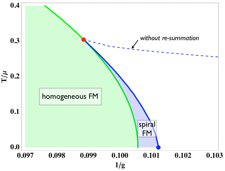
Figure 1: (color online) Phase diagram in $d=3$ as a function of inverse electron repulsion $1/g$ and temperature $T/\mu$. Above the tricritcal point (shown in red) we find a continuous transition between the ferromagnet at large $g$ and a paramagnet at small $g$. The spiral forms below the tricritical point between the paramagnet and the ferromagnet. The effect of the re-summation of leading divergencies is illustrated. (i) The dashed line shows the case without re-summation, which shows unphysical behavior as $T\to 0$ (ii) Using the re-summation of the leading divergences $\Delta F_{1}$, the spiral region becomes invisible on the scale of this phase diagram, collapsing into a region very close to the homogeneous magnetic state. (iii) The solid line shows the phase boundary of the spiral found using the form for $\Delta F$ in Eqn. (23), and gives the exact $T=0$ intercept, and the correct behaviour in the vicinity of the tricritical point.

The main effect of the re-summation is to cut off the $\ln T$-divergence by finite $M$. This fundamentally changes the behavior of the first-order spiral/paramagnet line as illustrated in Fig. 1. The phase boundary has a vertical intercept with the $T=0$ axis at a finite value $g_{\kappa}$, consistent with the Clausius-Clapeyron condition. Using just the leading re-summed expression $\Delta F_{1}(M)$ (20), we are left with a very narrow region of spiral order. However, we know that for small values of $T$, the sub-leading re-summed corrections will become significant, so we must include all the subleading corrections too. We may explicitly calculate the location of the $T=0$ intercept for the first-order spiral transition line, to find a critical coupling $1/g_{c}\sim 0.1012$. Previous Monte Carlo analysis Conduit et al. (2009) suggests the transition into the spiral state at $T=0$ will occur at $1/g\approx 0.133$. The numerical disagreement between the two approaches may stem from the fact that to carry out the $T=0$ Monte Carlo calculation, the contact interaction must be replaced by one with a negative finite range.

IV.2 Phase Diagram in $d=2$.

We proceed to calculate the phase diagram in $d=2$ by minimizing $\mathcal{F}(M,Q)=\mathcal{F}_{\textrm{mf}}(M,Q)+\Delta\mathcal{F}_{1}(M,Q)$ with $\mathcal{F}_{\textrm{mf}}$ given by Eq. (8) with $\langle\eta_{\mathbf{k}}^{2}\rangle=1/2$ and $\langle\eta_{\mathbf{k}}^{4}\rangle=3/8$ and $\Delta\mathcal{F}_{1}$ defined in Eq. (25). Note that since $\Delta\mathcal{F}_{1}$ is only known in the regimes $T\ll M$ and $T\gg M$ [see Eq. (25)], we will only be able to determine the asymptotic behavior of the phase boundaries and have to interpolate between the two regimes. There are crucial differences between the cases $d=2$ and $d=3$:

• In two dimensions, the density of states is constant, leading to an exponentially weak temperature dependence of $\alpha_{\textrm{mf}}$. As a consequence, the critical interaction strength $g_{c}(T)$ for the mean-field transition of the ferromagnet is practically constant up to $T\approx 0.2\mu$ [see Fig. 2a].

• The fluctuation contributions in $d=2$ are very different. Even in the vicinity of the tricritical point, we do not have a simple Landau expansion of the free energy; the corrections are intrinsically non-analytic across the whole phase diagram.

• The angular averages $\langle\eta_{\mathbf{k}}^{2n}\rangle$ are larger in $d=2$ and decay as $1/\sqrt{n}$ for large $n$, opposed to $1/n$ in $d=3$. This has a profound effect on how the free energy of the spiral relates to that of the homogeneous ferromagnet.

In spite of these differences, the phase diagram for the two-dimensional case turns out to be remarkably similar to that for three dimensions. We proceed to construct the phase diagram in three steps. i. We first analyze the effects of the fluctuation corrections $\Delta F_{1}(M)$ on the continuous transition between the ferromagnet and the paramagnet. This is controlled by the asymptotic form of $\Delta F_{1}$ in the regime $T\gg M$ since $M$ vanishes continuously at the second-order transition. ii. We determine the fluctuation-driven first-order transition, using the low temperature asymptotic form of $\Delta F_{1}$, which is valid for $T\ll M$. We extrapolate this first-order line to higher temperatures and estimate the position of the tricritical point. iii. We obtain the first-order spiral-to-paramagnet transition by minimizing $\mathcal{F}(M,Q)$ in the low-temperature regime. iv. Finally, we find that similar to the $d=3$ case, the Lifshitz line along which $Q\rightarrow 0$ coincides with the line $\alpha=0$. This line is again extrapolated up to the tricritical point.

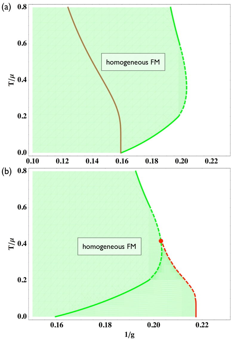
Figure 2: (color online) Intermediate phase diagrams in $d=2$ for $Q=0$. (a) Continuous phase boundaries between the ferromagnet and the paramagnet obtained from the condition $\alpha=0$, first using just the mean-field $\alpha=\alpha_{\textrm{mf}}$ (brown line), and then including the effects of fluctuations $\alpha=\alpha_{\textrm{mf}}+\alpha_{\textrm{fl}}$ (green line). In the regime $M\ll T\ll\mu$, $\alpha_{\textrm{fl}}=c_{+}T$ ($c_{+}<0$), leading to a stabilization of ferromagnet order. Around $T\simeq\mu$ fluctuations saturate, causing re-entrant behavior. We interpolate between the two regimes, indicated by a dashed green line. (b) The leading fluctuation correction $\Delta F_{1}(M)=c_{-}M^{3}\ln M$ in the regime $T\ll M$ causes a first-order transition at low temperatures (solid red line). The first-order line at higher temperatures is obtained by interpolation (dashed red line) to the tip of the re-entrant $\alpha=0$ line, where one expects the location of the tricritical point.

i. Second-Order Line. Using the asymptotic expression $\Delta F_{1}(M)=c_{+}M^{2}T$, valid for $\mu\gg T\gg M$, we obtain the fluctuation corrected transition line between the paramagnet and the ferromagnet by the condition $\alpha=\alpha_{\textrm{mf}}+c_{+}T=0$. Since $\alpha_{\textrm{mf}}$ is almost constant at low temperatures and since $c_{+}<0$, the region of stability of the ferromagnet increases with temperature where the phase boundary is almost linear. This is shown in Fig. 2a. At higher temperatures, the fluctuation effects saturate, and the second-order line then tracks the mean-field transition, albeit at lower values of $g$. We expect that the true second-order transition line interpolates between these two asymptotic limits, leading to the re-entrant behavior sketched in Fig. 2a.

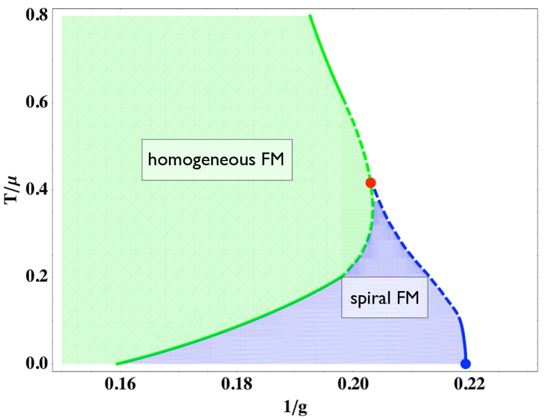
Figure 3: (color online) Phase diagram in $d=2$ as a function of inverse electron repulsion $1/g$ and temperature $T/\mu$. Dashed lines are interpolations between different asymptotic regimes. The phase diagram has the same topology as the one in $d=3$ (see Fig. 1) and exhibits a spiral phase below the tricritical point which is shown in red. As in $d=3$, the transition between the ferromagnet and the spiral is of the Lifshitz type while the spiral/paramagnet transition is first-order.

ii. First-Order Line. We now focus on the regime $T\ll M$ where the re-summed fluctuations are of the asymptotic form $\Delta F_{1}(M)=c_{-}M^{3}\ln M$ with $c_{-}>0$. This contribution leads to a first-order transition between the ferromagnet and the paramagnet at low temperatures and values of $g$ that are considerably smaller than those determined by the condition $\alpha=0$ for the second-order line. To determine the first-order phase boundary, we numerically search for solutions $M\neq 0$ of the equations $F(M)=0$ and $\partial_{M^{2}}F=0$. If we follow this first-order line to higher $T$, we expect a tricritical point at the intersection with the $\alpha=0$. The most likely scenario is that this point coincides with the tip of the re-entrant $\alpha=0$ line, sketched in Fig. 2b.

iii. Spiral Phase. Finally, we allow for states where $Q\neq 0$. As found previously, the Lifshitz line where $Q\rightarrow 0$ is given by the extension of the second-order ferromagnet-to-paramagnet transition line to temperatures below the tricritical point.lif

We continue to calculate the first-order, paramagnet-to-spiral transition line in the limit $T\to 0$, using the asymptotic form of $\Delta\mathcal{F}_{1}(M,Q)$ in the regime $T\ll M$ (25). We follow the same procedure we used in $d=3$ and first determine the optimal pitch $\tilde{Q}(M)$ for a given magnetization. This requires an expansion of $\mathcal{F}(M,Q)$ up to 4th order in $Q$. We then determine the first-order transition of $\tilde{F}(M)=\mathcal{F}(M,\tilde{Q}(M))$. As in the $3d$ case we find that this first-order transition pre-empts the one into the homogeneous state. From the asymptotic form of the free energy, we can only determine the phase boundary for small values of $T$ and rely on an interpolation up to the tricritical point. The resulting phase diagram is shown in Fig. 3.

V Conclusions and Discussion

Despite its apparent simplicity, the Hamiltonian (1) yields a rich and interesting phase diagram when we include the possibility of fluctuation-driven phases near to the ferromagnetic quantum critical point. Previous application of the quantum order-by-disorder approach to the three-dimensional caseConduit et al. (2009); Karahasanovic et al. (2012) showed that quantum fluctuations not only drive the transition first-order at low temperatures, but also stabilize an incommensurate spiral phase below the tricritical point. These results are valid in the vicinity of the tricritical point but fail for much smaller temperatures, where the phase behavior is no longer controlled by the smallness of the magnetization $M$ but instead by the leading divergences of all orders in $M$ as $T\to 0$.

In this work we have presented a detailed analysis of the non-analytic structure of the fluctuation corrections to the free energy in $d=2$ and $d=3$. We have demonstrated that there exists an underlying hierarchy of divergences and obtained closed-form expression for the re-summation of the leading terms of all orders in $M$. By adopting the fermionic quantum order-by-disorder approach and self-consistently expanding around an electronic state with a spiral magnetization, we have derived re-summed expressions for the free energy of the spiral ferromagnet. This re-summation of leading divergences allows us to track phase boundaries at low temperatures far away from the tricritical point.

Our results demonstrate that not only the fluctuation-driven first-order transitions but also the instabilities towards spiral order are generic features of itinerant ferromagnets. Despite the different non-analytic structures, we find very similar phase diagrams in $d=2$ and $d=3$. There are however differences which can be tested by future experiments. In $d=3$, the spiral phase is found in a narrow region on the border of ferromagnetism, leading to a sequence of transitions from paramagnet to spiral and finally to ferromagnet as temperature is decreased, consistent with recent experiments on PrPtAl (Ref. Jabbar et al., ). This order of transitions is not possible in $d=2$. Because of the re-entrant behavior of the phase boundary of the homogeneous ferromagnet, we predict that the spiral phase is located below the ferromagnetic state and stable over a larger region of the phase diagram.

Expressions for non-analytic contributions to the free energy have been previously obtained by diagrammatic methods.Belitz et al. (1997); Chubukov et al. (2004); Betouras et al. (2005); Rech et al. (2006); Efremov et al. (2008); Maslov and Chubukov (2009); Kirkpatrick and Belitz (2012) Our work shows that the diagrammatic calculations are equivalent to self-consistent second-order perturbation theory. In $d=3$, we indeed recover the previously-knownBelitz et al. (1999) result $\Delta F_{1}\sim M^{4}\ln(M^{2}+T^{2})$, and find the exact form of the $T=0$ free energy. This analytic form allows us to find the precise location of the quantum critical point for the ferromagnet in $3d$.

In $d=2$, we break new ground. In contrast to the three-dimensional case, a straightforward calculation of a Landau expansion for the free energy where each coefficient of $M^{2n}$ is a simple function of $T$ is not possible. This signposts the fact that the system is intrinsically non-analytic, even in the vicinity of the tricritical point. Indeed there is a lack of consensus on the form of the quantum corrections we should expect from diagrammatic work.Efremov et al. (2008); Kirkpatrick and Belitz (2012) In Ref. Kirkpatrick and Belitz, 2012, Belitz and Kirkpatrick argue that the fluctuation contributions are of the form $\Delta F\sim M^{2}\sqrt{M^{2}+T^{2}}$, which is in agreement with our result $\Delta F_{1}\sim M^{2}T$ in the regime $T\gg M$. However, the result of Ref. Kirkpatrick and Belitz, 2012 is based on the assumption that the singular behavior of the fluctuation integral for $T\ll M$ is cut off in the same way. Our work shows that this assumption is incorrect and that the asymptotic behavior for $T\ll M$ is given by $\Delta F_{1}\sim M^{3}\ln M$.

Our results lay the groundwork for studying the multi-critical behavior of itinerant ferromagnets. In $d=3$, the re-summed form for the phase diagram has already been used to study superconducting instabilities mediated by magnetic fluctuations.Conduit et al. (2013) In this instance, the intertwined magnetic spiral state and the superconducting instability resulted in the formation of a pair-density-wave state at very low temperatures. In two-dimensional systems such exotic states might be stabilized at higher temperatures since quantum fluctuations become more important and the resulting non-analyticities are of a different form. Future applications of the fermionic quantum order-by-disorder approach include the study of multiple-band effects, orbital fluctuations, and the competition between nesting instabilities and fluctuation-driven phase formation.

Appendix A Particle-hole density of states

In order to evaluate the fluctuation integral $\Delta F(M)$ (13), we must first calculate the particle-hole densities of states $\tilde{\rho}(q,\epsilon)$ and $\Delta\rho(q,\epsilon)$, which are defined in Eq. (12). We will do this separately for the cases $d=3$ and $d=2$.

A.1 Three dimensions

In $d=3$, and for $M=0$, $\tilde{\rho}$ takes the form

$$\begin{split}{\tilde{\rho}}(q,\epsilon)&=\int_{-1}^{1}d\cos\theta\int_{0}^{\infty}\frac{2\pi k^{2}dk}{(2\pi)^{3}}n\left(\frac{k^{2}}{2}+\frac{q^{2}}{8}-\frac{kq\cos\theta}{2}\right)\\ &\,\,\,\,\,\,\times\delta(\epsilon-kq\cos\theta).\end{split}$$ (27)

The integrals over $\cos\theta$ and $k$ may be done exactly. We are not so interested in the particle-hole densities themselves, but rather in their derivatives with respect to $\mu$, which enter the integrals $J_{n,n}$. For the $n$-th derivative we obtain

$$\partial^{n}_{\mu}{\tilde{\rho}}(q,\epsilon)={\tilde{\rho}}^{(n)}(q,\epsilon)=\frac{1}{(2\pi)^{2}q}\partial^{(n-1)}_{\mu}n\left[\phi^{-}(q,\epsilon)\right],$$ (28)

where we have defined

$$\phi^{\pm}(q,\epsilon)=\frac{1}{2}\left(\frac{\epsilon}{q}\pm\frac{q}{2}\right)^{2}.$$ (29)

Similarly, we find that

$$\Delta\rho^{(n)}(q,\epsilon)=\frac{1}{(2\pi)^{2}q}\partial^{(n-1)}_{\mu}\left\{n\left[\phi^{+}(q,\epsilon)\right]n\left[\phi^{-}(q,\epsilon)\right]\right\}.$$ (30)

A.2 Two Dimensions

In $d=2$, we must calculate the integral

$$\begin{split}{\tilde{\rho}}(q,\epsilon)&=\int_{0}^{2\pi}\,d\theta\int_{0}^{\infty}\frac{kdk}{(2\pi)^{2}}\,n\bigl{(}\frac{k^{2}}{2}+\frac{q^{2}}{8}-\frac{kq\cos{\theta}}{2}\bigr{)}\\ &\,\,\,\,\,\,\,\times\delta(\epsilon-kq\cos{\theta}).\end{split}$$ (31)

We carry out the $\theta$ integral to get

$${\tilde{\rho}}(q,\epsilon)=\frac{2}{(2\pi)^{2}}\int_{0}^{\infty}k\,dk\,\frac{n(\frac{k^{2}}{2}+\frac{q^{2}}{8}-\frac{\epsilon}{2})}{\sqrt{k^{2}q^{2}-\epsilon^{2}}}\theta(k^{2}q^{2}-\epsilon^{2}).$$ (32)

By a suitable change of variables, we reduce this to

$${\tilde{\rho}}(q,\epsilon)=\frac{\sqrt{2}}{(2\pi)^{2}q}\int_{0}^{\infty}\,\frac{dx}{\sqrt{x}}n[x+\phi^{-}(q,\epsilon)],$$ (33)

where the functions $\phi^{\pm}(q,\epsilon)$ are defined as before (29). An identical calculation for $\Delta\rho$ yields

$$\Delta\rho(q,\epsilon)=\frac{\sqrt{2}}{(2\pi)^{2}q}\int_{0}^{\infty}\,\frac{dx}{\sqrt{x}}n[x+\phi^{+}(q,\epsilon)]n[x+\phi^{-}(q,\epsilon)].$$ (34)

Although it is possible to perform the integrals (33) and (34) and write the results in terms of poly-logarithmic functions, the expressions in integral form will prove more useful to us.

Appendix B Calculation of $\Delta F_{1}(M)$ in $d=3$.

It is convenient to define a new function $\bar{n}(x)$ to keep our calculations uncluttered; this takes the form

$$\bar{n}(x)=\frac{1}{1+e^{x/T}}$$ (35)

and is a Fermi function with chemical potential $\mu=0$. The most divergent part of the integral $J_{n,n}$ in $d=3$ comes from

$$\begin{split}J_{n,n}&=\frac{2}{(2\pi)^{6}}\int\,\frac{dq\,d\epsilon_{1}\,d\epsilon_{2}}{(\epsilon_{1}+\epsilon_{2})}\delta^{(n-2)}[\phi^{-}(q,\epsilon_{1})-\mu]\\ &\,\,\,\,\,\,\times\delta^{(n-2)}[\phi^{-}(q,\epsilon_{2})-\mu]\bar{n}(\epsilon_{2}).\end{split}$$ (36)

We integrate by parts $(n-2)$ times each with respect to $\epsilon_{1}$ and $\epsilon_{2}$ to find

$$\begin{split}J_{n,n}&=\frac{2}{(2\pi)^{6}}\int\,\frac{q^{2n-2}}{k_{F}^{2n-2}}dq\,d\epsilon_{1}\,d\epsilon_{2}\biggl{(}\frac{\partial^{n-2}}{\partial\epsilon_{1}^{n-2}}\frac{\partial^{n-2}}{\partial\epsilon_{2}^{n-2}}\frac{1}{\epsilon_{1}+\epsilon_{2}}\biggr{)}\\ &\,\,\,\,\,\,\times\delta\left[\epsilon_{1}-\frac{q}{2}(q-2k_{F})\right]\delta\left[\epsilon_{2}-\frac{q}{2}(q-2k_{F})\right]\bar{n}(\epsilon_{2}),\end{split}$$ (37)

and use the $\delta$-functions to integrate over $\epsilon_{1}$ and $\epsilon_{2}$,

$$J_{n,n}=\frac{2(2n-4)!}{(2\pi)^{6}}\int_{-2k_{F}}^{\infty}\,d\delta q\frac{(2k_{F})^{2n-2}}{k_{F}^{2n-2}(2k_{F}\delta q)^{2n-3}}\bar{n}(k_{F}\delta q),$$ (38)

where $\delta q=q-2k_{F}$ is the deviation of the particle-hole pair’s momentum from $2k_{F}$, which is expected to be small. We simplify this equation by folding the integral around $\delta q=0$ and use the expression $\bar{n}(k_{F}\delta q)=\frac{1}{2}[1-\text{tanh}(k_{F}\delta q/2T)]$. The second term provides a cut-off for the lower limit of the integral, which now yields

$$J_{n,n}=\frac{-4(2n-4)!\nu_{F}^{3}}{(2\mu)^{2n-2}}\int_{\frac{T}{2\mu}}^{2}\frac{du}{u^{2n-3}},$$ (39)

where we have made a simple change of variables, $u=k_{F}\delta q$, and defined $\nu_{F}={k_{F}}/{2\pi^{2}}$. Substituting this expression into Eq. (17), we find

$$\Delta F_{1}=-64g^{2}\nu_{F}^{3}\mu^{2}\int_{\frac{T}{2\mu}}^{2}du\overset{\infty}{\underset{n=2}{\sum}}\frac{(2n-4)!(-1)^{n}(2gM)^{2n}}{(2n)!u^{2n-3}(2\mu)^{2n}}.$$ (40)

Taking sequential derivatives with respect to $M$, we simplify our expression significantly to obtain

$$\begin{split}\partial_{M}^{4}\Delta F_{1}&=-\frac{64g^{6}\nu_{F}^{3}}{\mu^{2}}\int_{\frac{T}{2\mu}}^{2}du\overset{\infty}{\underset{n=2}{\sum}}\frac{(-1)^{n}(2gM)^{2n-4}}{u^{2n-3}(2\mu)^{2n-4}}\\ &=-\frac{64g^{6}\nu_{F}^{3}}{\mu^{2}}\int_{\frac{T}{2\mu}}^{2}\,du\frac{u}{g^{2}M^{2}+u^{2}}\\ &=\frac{32g^{6}\nu_{F}^{3}}{\mu^{2}}\ln\left(\frac{g^{2}M^{2}}{\mu^{2}}+\frac{T^{2}}{4\mu^{2}}\right).\end{split}$$ (41)

To get $\Delta F_{1}$, we integrate this four times with respect to $M$, keeping only terms that will give us an overall coefficient of $M^{4}$. This gives the final closed form expression

$$\Delta F_{1}(M,T)=\frac{4g^{6}\nu_{F}^{3}M^{4}}{3\mu^{2}}\ln\left(\frac{g^{2}M^{2}}{\mu^{2}}+\frac{T^{2}}{4\mu^{2}}\right)$$ (42)

for the re-summation of leading divergences in $d=3$.

Appendix C Calculation of $\Delta F(M)$ in $d=3$.

We wish to use the recursion relation given in the text  (19) to calculate the complete, all-orders re-summation at $T=0$. Firstly, we write $\Delta F_{1}$ in terms of the variable $y=\sqrt{2}\mu/gM$, and define the functions $f_{n}(y)$ by

$$\Delta F_{n}(M)=(gM)^{2}f_{n}(y).$$ (43)

In terms of this new variable, the recursion relation  (19) takes the form

$$f_{n}(y)=\frac{1}{n!}\partial_{y}^{2n-2}f_{1}(y).$$ (44)

By Fourier transforming this expression to $k$-space, and after summation over $n$, we find that $\Delta F=\underset{n}{\sum}\Delta F_{n}$ is given by

$$\Delta\tilde{F}(k)=g^{2}M^{2}\frac{1-e^{-k^{2}}}{k^{2}}{\tilde{f}}_{1}(k).$$ (45)

We approximate the Fourier transform of $(1-e^{-k^{2}})/k^{2}$ by a triangular function with the same total area, to do the convolution and approximate for $y\gg 1$. Expressing the result in terms of $M$, we find the full resummation of the $T=0$ quantum corrections to all orders, which is given by

$$\Delta F(M)=2\sqrt{\pi}\lambda M^{4}\ln\biggl{[}\frac{g^{2}M^{2}}{\mu^{2}}\biggr{]}.$$ (46)

Appendix D Calculation of $\Delta F_{1}(M)$ in $d=2$.

Using the integral expressions (33) and (34) for the particle-hole densities of states in $d=2$, $J_{n,n}$ is given by a five-dimensional integral

$$\begin{split}J_{n,n}&=\frac{2}{(2\pi)^{5}}\int\,\frac{dq}{q}d{\epsilon}_{1}\,d{\epsilon}_{2}\,dx\,dy\partial_{\mu}^{n}n[x+\phi^{-}(q,\epsilon_{1})]\\ &\,\,\,\,\,\times\frac{\partial_{\mu}^{n}\left\{n[y+\phi^{-}(q,\epsilon_{2})]n[y+\phi^{+}(q,\epsilon_{2})]\right\}}{\sqrt{xy}(\epsilon_{1}+\epsilon_{2})},\end{split}$$ (47)

where $\phi^{\pm}(q,\epsilon)$ are defined as before and the ranges of integration are $\epsilon_{1},\epsilon_{1}\in(-\infty,\infty)$ and $q,x,y\in[0,\infty)$.

In order to do the integrals over $\epsilon_{1}$ and $\epsilon_{2}$, we first focus on the most divergent term, where all the derivatives hit the second Fermi function, and none hit the third. We make the same approximation as before, namely that $n^{\prime}(x)=-\delta(x-\mu)$, and then linearize the arguments of the derivatives of the Fermi functions as for $d=3$. We write the derivatives with respect to argument in terms of derivatives with respect to $\epsilon$, and then integrate by parts with respect to $\epsilon_{1}$ and $\epsilon_{2}$, $(n-1)$ times each. This gives

$$\begin{split}J_{n,n}&=\frac{2(2n-2)!}{(2\pi)^{5}}\int\frac{dq}{q}\,d{\epsilon}_{1}\,d{\epsilon}_{2}\,dx\,dy\frac{\bar{n}(\epsilon_{2})}{\sqrt{xy}(\epsilon_{1}+\epsilon_{2})^{2n-1}}\\ &\times\frac{q^{2n}}{k_{F}^{2n}}\delta(y-k_{F}\epsilon_{2}/q+k_{F}\delta q)\delta(x-k_{F}\epsilon_{1}/q+k_{F}\delta q).\end{split}$$ (48)

After these approximations, the integrals over $\epsilon_{1}$ and $\epsilon_{2}$ are trivial and we obtain

$$\begin{split}J_{n,n}&=\frac{2(2n-2)!}{(2\pi)^{5}k_{F}}\int_{-2k_{F}}^{\infty}\,d\delta q\int_{0}^{\infty}dx\int_{0}^{\infty}dy\frac{1}{\sqrt{xy}}\\ &\,\,\,\,\,\times\frac{\bar{n}(2y+k_{F}\delta q)}{(x+y+2k_{F}\delta q)^{2n-1}}\end{split}$$ (49)

with $\delta q=q-2k_{F}$ as before. We now feed this back into the re-summation expression (17), and simplify by taking two $M$-derivatives,

$$\begin{split}\partial_{M}^{2}\Delta F_{1}&=\frac{-32g^{4}}{(2\pi)^{5}k_{F}}\int_{-2k_{F}}^{\infty}d\delta q\int_{0}^{\infty}dx\int_{0}^{\infty}dy\frac{1}{\sqrt{xy}}\\ &\,\,\,\,\,\,\,\times\frac{x+y+k_{F}\delta q}{4g^{2}M^{2}+(x+y+k_{F}\delta q)^{2}}\bar{n}(2y+k_{F}\tilde{q}).\end{split}$$ (50)

Changing variables $u=y+k_{F}\delta q$ and doing the integral over $x$ we get

$$\begin{split}\partial_{M}^{2}\Delta F_{1}&=\frac{-32g^{4}}{(2\pi)^{5}k_{F}}\frac{\pi}{\sqrt{2}}\int_{-2k_{F}^{2}}^{\infty}du\int_{0}^{\infty}dy\frac{1}{\sqrt{y}}\\ &\,\,\,\,\,\times\sqrt{\frac{\sqrt{u^{2}+4g^{2}M^{2}}+u}{u^{2}+4g^{2}M^{2}}}\bar{n}(y+u).\end{split}$$ (51)

We now do the $y$-integral to get

$$\begin{split}\partial_{M}^{2}\Delta F_{1}&=\frac{32g^{4}\pi^{3/2}\sqrt{T}}{(2\pi)^{5}\sqrt{2}k_{F}}\int_{-4\mu}^{\infty}du\,\text{Li}_{1/2}(-e^{-u/T})\\ &\,\,\,\,\,\,\times\sqrt{\frac{\sqrt{u^{2}+4g^{2}M^{2}}+u}{u^{2}+4g^{2}M^{2}}}.\end{split}$$ (52)

Since this integration cannot be done analytically, we approximate it in two limits. Firstly, when $T\gg M$ we take $M=0$ inside Eq. (52), which becomes

$$\partial_{M}^{2}\Delta F_{1}=\frac{32g^{4}\pi^{3/2}\sqrt{2T}}{(2\pi)^{5}\sqrt{2}k_{F}}\int_{-4\mu}^{\infty}\frac{du}{\sqrt{u}}\text{Li}_{1/2}(-e^{-u/T}).$$ (53)

Only positive values of $u$ contribute to this integral when taking the limit $T\rightarrow 0$; the lower limit becomes $u=0$. We may then scale out $T$ to get

$$\partial_{M}^{2}\Delta F_{1}=\frac{32g^{4}\pi^{3/2}T}{(2\pi)^{5}k_{F}}\int_{0}^{\infty}\frac{du}{\sqrt{u}}\times\text{Li}_{1/2}(-e^{-u}).$$ (54)

We split the integral into two regions, $u\in[0,1]$ where we approximate $\text{Li}_{1/2}(-e^{-u/T})\approx\text{Li}_{1/2}(-1)$ and $u\in[1,\infty)$ where $\text{Li}_{1/2}(-e^{-u/T})\approx 0$ to give

$$\partial_{M}^{2}\Delta F_{1}=\frac{64g^{4}\pi^{3/2}T}{(2\pi)^{5}k_{F}}\text{Li}_{1/2}(-1),$$ (55)

which corresponds to a term in the free energy

$$\Delta F_{1}(M)=\frac{16\sqrt{2}g^{4}\pi^{3/2}\text{Li}_{1/2}(-1)}{(2\pi)^{5}}M^{2}T.$$ (56)

Next, we turn our attention to the limit where $T\ll M$. Setting $T=0$ in Eq. (52), we now see that only values of $u<0$ contribute. For this range of $u$, we may approximate the poly-logarithm by $\text{Li}_{n}(-e^{u})\sim u^{n}/\Gamma(n+1)$ where $\Gamma$ is the Euler gamma function. This gives

$$\begin{split}\partial_{M}^{2}\Delta F_{1}&=\frac{-32g^{4}\pi^{3/2}}{(2\pi)^{5}\sqrt{2}k_{F}\Gamma(3/2)}\\ &\,\,\,\,\,\times\int_{0}^{4\mu}du\sqrt{\frac{u\sqrt{u^{2}+4g^{2}M^{2}}-u^{2}}{u^{2}+4g^{2}M^{2}}}.\end{split}$$ (57)

We rescale $u=2M\tilde{u}$, and scale out $\mu$ to get

$$\begin{split}\partial_{M}^{2}\Delta F_{1}&=\frac{-32g^{4}\pi^{3/2}M}{(2\pi)^{5}\Gamma(3/2)}\\ &\times\int_{0}^{2/M}d\tilde{u}\sqrt{\frac{\tilde{u}\sqrt{{\tilde{u}}^{2}+g^{2}}-{\tilde{u}}^{2}}{{\tilde{u}}^{2}+g^{2}}}.\\ \end{split}$$ (58)

Splitting the integral as before, and approximating the two halves we find

$$\begin{split}&\int_{0}^{2/M}d\tilde{u}\sqrt{\frac{\tilde{u}\sqrt{{\tilde{u}}^{2}+g^{2}}-{\tilde{u}}^{2}}{{\tilde{u}}^{2}+g^{2}}}\\ &\approx\int_{0}^{1}d\tilde{u}\sqrt{\frac{\tilde{u}\sqrt{{\tilde{u}}^{2}+g^{2}}-{\tilde{u}}^{2}}{{\tilde{u}}^{2}+g^{2}}}+\int_{1}^{2/M}d\tilde{u}\frac{1}{\sqrt{{\tilde{u}}^{2}+g^{2}}}.\end{split}$$ (59)

The first term gives us a numerical constant, which corresponds to a sub-leading $\partial_{M}^{2}\Delta F_{1}\sim M$ piece. The second integral gives us $\text{ArcSinh}(2/M)-\text{ArcSinh}(1)$. Recall that $\text{ArcSinh}(x)=\ln(x+\sqrt{x^{2}+1})$, and that we are working in the limit where $M<1$, then this first, positive term gives us a leading contribution

$$\partial_{M}^{2}\Delta F_{1}=\frac{32g^{4}\pi^{3/2}}{(2\pi)^{5}\Gamma(3/2)}M\ln M,$$ (60)

which corresponds to the term

$$\Delta F_{1}(M)=\frac{16g^{4}\pi^{3/2}}{(2\pi)^{5}\Gamma(3/2)}M^{3}\ln M,$$ (61)

in the free energy for sufficiently small values of $T$.

References

- Hertz (1976) J. A. Hertz, Physical Review B 14, 1165 (1976).
- Moriya (1985) T. Moriya, Spin Fluctuations in Itinerant Electron Magnetism (Springer Verlag, Berlin, 1985).
- Millis (1993) A. Millis, Physical Review B 48, 7183 (1993).
- Belitz et al. (1997) D. Belitz, T. R. Kirkpatrick, and T. Vojta, Phys. Rev. B 55, 9452 (1997).
- Belitz et al. (1999) D. Belitz, T. R. Kirkpatrick, and T. Vojta, Phys. Rev. Lett. 82, 4707 (1999).
- Chubukov et al. (2004) A. V. Chubukov, C. Pépin, and J. Rech, Phys. Rev. Lett. 92, 147003 (2004).
- Betouras et al. (2005) J. Betouras, D. Efremov, and A. Chubukov, Phys. Rev. B 72, 115112 (2005).
- Rech et al. (2006) J. Rech, C. Pépin, and A. V. Chubukov, Phys. Rev. B 74, 195126 (2006).
- Efremov et al. (2008) D. V. Efremov, J. J. Betouras, and A. Chubukov, Phys. Rev. B 77, 220401 (2008).
- Maslov and Chubukov (2009) D. L. Maslov and A. V. Chubukov, Phys. Rev. B 79, 075112 (2009).
- Kirkpatrick and Belitz (2012) T. R. Kirkpatrick and D. Belitz, Phys. Rev. B 85, 134451 (2012).
- Belitz et al. (2001) D. Belitz, T. R. Kirkpatrick, M. T. Mercaldo, and S. L. Sessions, Phys. Rev. B 63, 174428 (2001).
- Pfleiderer et al. (2001) C. Pfleiderer, S. R. Julian, and G. G. Lonzarich, Nature 414, 427 (2001).
- Uemura et al. (2007) Y. J. Uemura, T. Goko, I. M. Gat-Malureanu, J. P. Carlo, P. L. Russo, A. T. Savici, A. Aczel, G. J. MacDougall, J. A. Rodriguez, G. M. Luke, et al., Nature Physics 3, 29 (2007).
- Otero-Leal et al. (2008) M. Otero-Leal, F. Rivadulla, M. Garcia-Hernandez, A. Pineiro, V. Pardo, D. Baldomir, and J. Rivas, Phys. Rev. B 78, 180415(R) (2008).
- Taufour et al. (2010) V. Taufour, D. Aoki, G. Knebel, and J. Flouquet, Phys. Rev. Lett. 105, 217201 (2010).
- Yelland et al. (2011) E. A. Yelland, J. M. Barraclough, W. Wang, K. V. Kamenev, and A. D. Huxley, Nature Physics 7, 890 (2011).
- Conduit et al. (2009) G. J. Conduit, A. G. Green, and B. D. Simons, Phys. Rev. Lett. 103, 207201 (2009).
- Karahasanovic et al. (2012) U. Karahasanovic, F. Krüger, and A. G. Green, Phys. Rev. B 85, 165111 (2012).
- Berridge et al. (2009) A. M. Berridge, A. G. Green,, S. A. Grigera and B. D. Simons, Phys. Rev. Lett. 102, 136404 (2009).
- Berridge et al. (2010) A. M. Berridge, S. A. Grigera, B. D. Simons and A. G. Green, Phys. Rev. B 81, 054429 (2010).
- Igoshev et al. (2012) P. A. Igoshev, A. V. Zarubin, A. A. Katanin and V. Yu. Irkhin, J. Magn. Magn. Matt. 324, 3601 (2012).
- Katanin et al. (2011) A. A. Katanin, H. Yamase, and V. Yu. Irkhin, J. Phys. Soc. Jpn. 80, 063702 (2011).
- Igoshev2 et al. (2011) P. A. Igoshev, V. Yu. Irkhin, and A. A. Katanin, Phys. Rev. B 83, 245118 (2011).
- Moriya (1960) T. Moriya, Phys. Rev 120, 1, 91 (1960).
- Dzyaloshinsky (1958) I. Dzyaloshinsky, J. Phys. Chem. Solids 4, 4, 241 (1958).
- Bak et al. (1980) P. Bak and M. H. Jensen, J. Phys. C. 13, 31 L881 (1980).
- Krüger et al. (2012) F. Krüger, U. Karahasanovic, and A. G. Green, Phys. Rev. Lett. 108, 067003 (2012).
- Coleman and Weinberg (1973) S. Coleman and E. Weinberg, Phys. Rev. D 7, 1888 (1973).
- Casimir and Polder (1948) H. B. G. Casimir and D. Polder, Phys. Rev. 73, 360 (1948).
- Villain, J. et al. (1980) Villain, J., Bidaux, R., Carton, J.-P., and Conte, R., J. Phys. France 41, 1263 (1980).
- Chandra et al. (1990) P. Chandra, P. Coleman, and A. I. Larkin, Phys. Rev. Lett. 64, 88 (1990).
- Mila et al. (1991) F. Mila, D. Poilblanc, and C. Bruder, Phys. Rev. B 43, 7891 (1991).
- Zaanen (2000) J. Zaanen, Phys. Rev. Lett. 84, 753 (2000).
- Krüger and Scheidl (2006) F. Krüger and S. Scheidl, Europhys. Lett. 74, 896 (2006).
- (36) G. Jabbar, D. A. Sokolov, D. Wermeille, C. Stock, F. Dremmel, F. Krüger, A. G. Green, and A. Huxley, unpublished.
- Thomson et al. (2013) S. J. Thomson, F. Krüger, and A. G. Green, Phys. Rev. B 87, 224203 (2013).
- Lausberg et al. (2012) S. Lausberg, A. Hannaske, A. Steppke, L. Steinke, T. Gruner, C. Krellner, C. Klingner, M. Brando, C. Geibel, and F. Steglich, Phys. Rev. Lett. 109, 216402 (2012).
- (39) R. K. Pathria, Statistical mechanics, (Butterworth-Heinemann, Oxford/Boston, 1996).
- von Keyserlingk and Conduit (2013) C. W. von Keyserlingk and G. J. Conduit, Phys. Rev. B 87, 184424 (2013).
- (41) The double factorial function is defined for odd argument as and for even argument as .
- (42) Recall that we define the “optimal” for a given as which solves the equation . Using Eq. (8), we see that this translates into . Taking the limit that in this expression, and assuming that the angular average is non-zero, we find that this reduces to the expression , which is the condition that . Therefore, the Lifshitz line for the spiral coincides with the extension of the second-order line below .
- (43) By doing the re-summation for , we remove one of the two energy scales in the problem completely. As a result, we cannot garner any information about the precise nature of the relative scaling between and that would be imposed on us by doing the complete re-summation for .
- Conduit et al. (2013) G. J. Conduit, C. J. Pedder, and A. G. Green, Phys. Rev. B 87, 121112 (2013).