On the consistency of MPS

Abstract

The consistency of Moving Particle Semi-implicit (MPS) method in reproducing the gradient, divergence and Laplacian differential operators is discussed in the present paper. Its relation to the Smoothed Particle Hydrodynamics (SPH) method is rigorously established. The application of the MPS method to solve the Navier-Stokes equations using a fractional step approach is treated, unveiling inconsistency problems when solving the Poisson equation for the pressure. A new corrected MPS method incorporating boundary terms is proposed. Applications to one dimensional boundary value Dirichlet and mixed Neumann-Dirichlet problems and to two-dimensional free-surface flows are presented.

, , , ,

1 Introduction

The “Moving Particle Semi-implicit” method (MPS) is a numerical technique first introduced by Koshizuka and Oka in the nineties (Koshizuka et al., 1995; Koshizuka and Oka, 1996) to solve incompressible Navier-Stokes equations. It relies on a meshless discretization of the continuum to approximate differential operators. In order for the obtained flow field to exhibit the properties of an incompressible flow, a fractional time step approach is used. This approach requires solving a Poisson equation for the pressure field at every time step, which consequently demands a numerical approximation of the Laplacian operator.

The MPS scheme is mainly used to solve violent free-surface flows, exploiting the fact that no mesh is needed for the computations. This can be seen in (Koshizuka et al., 1998) where the technique was used to simulate breaking waves on a sloping beach and in (Khayyer and Gotoh, 2009a, b) where impact pressures in sloshing flows are accurately computed. Yoon et al. (1999a) extended MPS method to simulate multiphase flows and Yoon et al. (1999b) improved the MPS formulation in regards to the advection scheme by incorporating an arbitrary Lagrangian-Eulerian model.

With the increasing computational power in the early 2000s, Naito and Sueyoshi (Naito and Sueyoshi, 2001; Sueyoshi and Naito, 2003) extended the method to 3D. They utilized it to simulate complex marine engineering problems, such as the sinking of a vessel after the flooding of the cargo holds and green water events. Tsukamoto et al. (2011) adapted the MPS method to model complex fluid structure interaction problems. Different corrections aimed at improving the accuracy of the method have recently been documented. Tanaka and Masunaga (2010) introduced some corrections in the fractional step pressure solver in order to mitigate pressure oscillations. Khayyer and Gotoh (2011) enhanced the capabilities of the method in order to better approximate tensile states in fluids and developed a higher order approximation to the differential operators aiming at obtaining more accurate pressure fields Khayyer and Gotoh (2010, 2012); the improvement is demonstrated with results for sloshing flows both in two and three dimensional cases.

Regardless all that body of work neither the derivation of the MPS numerical method from its first principles, nor its consistency in regards to how accurately it reproduces the continuum as the numerical resolution increases, have been discussed at length in the literature. As CFD practitioners we believe this issue is paramount in order to guarantee the Engineering applicability of the numerical technique.

The present paper addresses this matter by first analyzing the consistency of the MPS approximations to the gradient, divergence and Laplacian operators and deriving continuous integral forms of these approximations. Second, the connections with Smoothed Particle Hydrodynamics (SPH), see e.g. (Monaghan, 2012), are rigorously presented by relating, through the integral form of the operators, the MPS weighting function with the SPH kernel. Third, the integral form of the operators is applied to the solution of the Poisson equation used in MPS for the pressure computation through the fractional step methodology. Some problematic issues regarding the implementation of Dirichlet and Neumann boundary conditions are discussed and some corrections to the operators proposed. Finally, applications to one-dimensional problems and two-dimensional free-surface flows are presented.

2 Governing equations

Newtonian incompressible flows are the ones treated with the MPS method. The incompressible Navier-Stokes equations in Lagrangian formalism are hence taken as the field equations:

$$\frac{D\mathbf{r}}{Dt}\,= \,\mathbf{u},$$ (1)

$$\displaystyle{\nabla\cdot}\mathbf{u}\,= \,0,$$ (2)

$$\displaystyle{\frac{D\mathbf{u}}{Dt}}\,=$$

where $\rho$ stands for the fluid density and $\mathbf{g}$ is a generic external volumetric force field. The flow velocity $\mathbf{u}$ is defined as the material derivative of a fluid particle with position $\mathbf{r}$. $\varmathbb{T}$ denotes the stress tensor of a Newtonian incompressible fluid:

$$\varmathbb{T}\,=-P\,\boldsymbol{\mathit{I}}\,+\,2\,\mu\,\varmathbb{D}\,,$$ (3)

in which $P$ is the pressure, $\varmathbb{D}$ is the rate of deformation tensor $(\varmathbb{D}=(\nabla\mathbf{u}+\nabla\mathbf{u}^{T})/2)$ and $\mu$ is the dynamic viscosity. With this notation, the divergence of the stress tensor $\varmathbb{T}$ is computed as:

$$\nabla\cdot\varmathbb{T}\,=\,-\,\nabla P\,+\,\mu\nabla^{2}\mathbf{u}\,.$$ (4)

The MPS method is based on a Helmholtz-Hodge decomposition of an intermediate velocity field initially devised by Chorin (Chorin, 1968) in the late sixties. First, an intermediate velocity field $\mathbf{u^{*}}$ is explicitly computed using the momentum equation but ignoring the pressure term. Second, the zero divergence condition is imposed on the velocity field at the next time step, thus obtaining the Poisson equation for the pressure:

$$\nabla^{2}P=\frac{\rho}{\Delta t}\left(\nabla\cdot\mathbf{u^{*}}\right),$$ (5)

in which $\Delta t$ is the time step. Once the pressure is found, pressure gradients and particle positions are modified. A comprehensive flow-chart of the whole approach can be found in e.g. (Yoon et al., 1999b).

3 MPS discretization

3.1 Density and number density

The set of equations (1-LABEL:Navier_Stokes_inc) has to be discretized in order to implement the fractional step algorithm. The fluid domain is discretized in a set of particles and the differential operators at an individual particle $i$ are evaluated using the value of the different fields at the neighboring particles. The MPS method weights these neighboring particle properties by using a compactly supported function $w$ whose argument is the distance between particles $\left|\mathbf{x}_{i}-\mathbf{x}_{j}\right|$ normalized with the cut-off radius $r_{e}$ and which is non-negative. The weighting function is singular at the origin in some formulations (Koshizuka and Oka, 1996; Tsukamoto et al., 2011; Khayyer and Gotoh, 2011) and regular in others (Yoon et al., 1999b, a). The notation of reference (Yoon et al., 1999b) is used to present the formalism.

A particle number density at a particle with coordinates $\mathbf{x}_{i}$ is defined as:

$$\langle n\rangle_{i}:=\sum_{j\in J_{i}}w\left(\frac{\left|\mathbf{x}_{i}-\mathbf{x}_{j}\right|}{r_{e}}\right),$$ (6)

where $J_{i}$ consists in all neighboring particles’ indexes and it may or may not include $i$ itself (Yoon et al., 1999a, b).

In the MPS literature, only the dependance of $w$ on the distance $\left|\mathbf{x}_{i}-\mathbf{x}_{j}\right|$ is made explicit in the notation. However, the definition of the weighting function incorporates the cut-off radius $r_{e}$ in terms of the ratio $\left|\mathbf{x}\right|/r_{e}$. We have chosen to make explicit the dependance of the weighting function on $r_{e}$; the benefits of this choice, which is non-standard in the MPS literature, will be clear in the computations that follow.

The approximation to the density field for a particle $i$ is obtained from $\langle n\rangle_{i}$ as (Yoon et al., 1999b):

$$\langle\rho\rangle_{i}=\frac{m\langle n\rangle_{i}}{\int_{\mathbb{R}^{d}}w\left(\frac{\left|\mathbf{x}\right|}{r_{e}}\right)\,d\mathbf{x}},$$ (7)

where $m$ is the mass of each particle and $d$ is the number of dimensions.

Since we are solving incompressible flows, the fluid has its constant reference density $\rho_{0}$ as a fundamental physical magnitude, for which a compatible reference number density $n_{0}$ can be defined from equation (7) as:

$$n_{0}=\frac{\rho_{0}}{m}\,\int_{\mathbb{R}^{d}}w\left(\frac{\left|\mathbf{x}\right|}{r_{e}}\right)\,d\mathbf{x}.$$ (8)

The mass of a particle $m$ can be obtained as the total mass of the fluid $M$ divided by the number of particles $N$. Moreover, the volume integral of the kernel in equation (8) equals, by defining $\mathbf{q}=\mathbf{x}/r_{e}$:

$$\int_{\mathbb{R}^{d}}w\left(\frac{\left|\mathbf{x}\right|}{r_{e}}\right)\,d\mathbf{x}=\left(r_{e}\right)^{d}\int_{\mathbb{R}^{d}}w\left(\left|\mathbf{q}\right|\right)\,d\mathbf{q}.$$ (9)

Let us define $A_{0}$ as

$$A_{0}=\int_{\mathbb{R}^{d}}w\left(\left|\mathbf{q}\right|\right)\,d\mathbf{q}.$$ (10)

This value only involves the shape of the kernel and does not depend on the number of particles nor does it depend on the specific value of $r_{e}$. Using this notation, equation (8) becomes:

$$n_{0}=\frac{\rho_{0}}{(M/N)}\,\left(r_{e}\right)^{d}\,A_{0}.$$ (11)

The ratio $M/\rho$ of the total mass over the density is the total volume $V$. Therefore,

$$n_{0}=\frac{1}{(V/N)}\,\left(r_{e}\right)^{d}\,A_{0}.$$ (12)

The total volume over the number of particles, $V/N$, is the volume $\upsilon$ associated to each particle. Let us call $\Delta x$ the typical particle spacing. It can be assumed that $\upsilon=\left(\Delta x\right)^{d}$ and with this in mind the value $n_{0}$ satisfies

$$\frac{1}{n_{0}}=\frac{1}{A_{0}}\left(\frac{\Delta x}{r_{e}}\right)^{d}.$$ (13)

This expression will be useful in the computations that follow.

The ratio $r_{e}/\Delta x$ is an indicator of the number of particles inside the weighting function support (neighbors).

Identity (13) is important because it allows for the introduction of the typical particle distance $\Delta x$ in the formalism. The integral version of the MPS differential operators is obtained by taking the limit as $\Delta x\rightarrow 0$.

3.2 Gradient and divergence

The gradient in the MPS method for a scalar function $\phi$ at a particle with co-ordinates $\mathbf{x}_{i}$ is approximated (see e.g. (Yoon et al., 1999b)) by the following sum

$$\langle\nabla\phi\rangle_{i}=\frac{d}{n_{0}}\sum_{j\neq i}\left[\frac{\phi_{j}-\phi_{i}}{{\left|\mathbf{x}_{j}-\mathbf{x}_{i}\right|^{2}}}\left(\mathbf{x}_{j}-\mathbf{x}_{i}\right)w\left(\frac{\left|\mathbf{x}_{j}-\mathbf{x}_{i}\right|}{r_{e}}\right)\right].$$ (14)

This sum can be interpreted as a discrete approximation of an integral. Taking into account the value of $n_{0}$ given by equation (13) a continuum analogue of the MPS discrete gradient is defined by:

$$\left\langle\partial_{x_{k}}\phi\right\rangle\left(\mathbf{x}\right)\approx\frac{d}{\left(r_{e}\right)^{d}A_{0}}\int_{\mathbb{R}^{d}}\frac{\phi(\mathbf{x^{\prime}})-\phi(\mathbf{x})}{{\left|\mathbf{x^{\prime}}-\mathbf{x}\right|^{2}}}\left(x^{\prime}_{k}-x_{k}\right)w\left(\frac{\left|\mathbf{x}-\mathbf{x^{\prime}}\right|}{r_{e}}\right)d\mathbf{x^{\prime}}.$$ (15)

The question arises whether this expression is a consistent approximation to the gradient of a function. It is possible to compare it with the SPH expression of the gradient (see section A.4 in the appendix), whose consistency has been established in the literature (see appendix for details). Let us rewrite (15) as:

$$\left\langle\partial_{x_{k}}\phi\right\rangle\left(\mathbf{x}\right)\approx-\frac{d}{\left(r_{e}\right)^{d}A_{0}}\int_{\mathbb{R}^{d}}\frac{\phi(\mathbf{x^{\prime}})-\phi(\mathbf{x})}{{\left|\mathbf{x}-\mathbf{x^{\prime}}\right|}}\left(x_{k}-x^{\prime}_{k}\right)\frac{1}{{\left|\mathbf{x}-\mathbf{x^{\prime}}\right|}}w\left(\frac{\left|\mathbf{x}-\mathbf{x^{\prime}}\right|}{r_{e}}\right)d\mathbf{x^{\prime}}.$$ (16)

If expressions (16) and (98) in the appendix were to coincide for every function $\phi$, necessarily, the following relation between the SPH kernel and the given MPS weighting function must hold:

$$\frac{1}{h^{d+1}}\tilde{W}^{\prime}\left(\frac{\left|\mathbf{x}\right|}{h}\right)=-\frac{d}{\left(r_{e}\right)^{d}A_{0}}\frac{1}{{\left|\mathbf{x}\right|}}w\left(\frac{\left|\mathbf{x}\right|}{r_{e}}\right).$$ (17)

Assuming that the MPS weighting function and the SPH kernel characteristic lengths are equal ($h\equiv r_{e}$), we have

$$\mathbf{q}=\frac{\mathbf{x}}{r_{e}}=\frac{\mathbf{x}}{h}.$$

SPH practitioners usually consider kernels with a $2h$ support radius whilst the radius of the MPS weighting function is $r_{e}$. Nonetheless, for the sake of simplicity, we will assume that both are equal.

Set $q:=\left|\mathbf{q}\right|$; equation (17) can then be rewritten as:

$$\tilde{W}^{\prime}(q)=-\frac{d}{A_{0}}\frac{1}{q}w(q).$$ (18)

This expression can be used to obtain the function $\tilde{W}$ involved in the definition of the SPH kernel from the MPS weighting function $w$. However, in order for equation (18) to give rise to a well defined SPH kernel, we must first check that:

$$\int_{\mathbb{R}^{d}}\tilde{W}\left(\left|\mathbf{q}\right|\right)d\mathbf{q}=1.$$ (19)

This is indeed the case since combining equations (10), (18) and (94) from the appendix, we deduce that

$$\int_{\mathbb{R}^{d}}\tilde{W}(\left|\mathbf{q}\right|)d\mathbf{q}=-\frac{1}{d}\int_{\mathbb{R}^{d}}\left|\mathbf{q}\right|\tilde{W}^{\prime}(\left|\mathbf{q}\right|)d\mathbf{q}=\frac{1}{A_{0}}\int_{\mathbb{R}^{d}}w(\left|\mathbf{q}\right|)d\mathbf{q}=1.$$

Let us now focus on the divergence operator, with $\mathbf{u}$ being a generic vector field. The divergence of $\mathbf{u}$ at a particle with co-ordinates $\mathbf{x}_{i}$ is computed through the MPS method (see e.g. (Yoon et al., 1999b)) with the following sum:

$$\langle\nabla\cdot\mathbf{u}\rangle=\frac{d}{n_{0}}\sum_{j\neq i}\left[\frac{\left(\mathbf{u}_{j}-\mathbf{u}_{i}\right)\cdot\left(\mathbf{x}_{j}-\mathbf{x}_{i}\right)}{{\left|\mathbf{x}_{j}-\mathbf{x}_{i}\right|^{2}}}w\left(\frac{\left|\mathbf{x}_{j}-\mathbf{x}_{i}\right|}{r_{e}}\right)\right].$$ (20)

Substituting $n_{0}$ with its value from equation (13) and interpreting the sum as a discrete approximation of an integral, we get a continuum analogue of the MPS discrete divergence:

$$\left\langle\nabla\cdot\mathbf{u}\right\rangle\left(\mathbf{x}\right)\approx\frac{d}{\left(r_{e}\right)^{d}A_{0}}\int_{\mathbb{R}^{d}}\frac{\left(\mathbf{u^{\prime}}-\mathbf{u}\right)\cdot\left(\mathbf{x^{\prime}}-\mathbf{x}\right)}{{\left|\mathbf{x^{\prime}}-\mathbf{x}\right|^{2}}}w\left(\frac{\left|\mathbf{x}-\mathbf{x^{\prime}}\right|}{r_{e}}\right)d\mathbf{x^{\prime}}.$$ (21)

Equation 21 can be rewritten as:

$$\left\langle\nabla\cdot\mathbf{u}\right\rangle\left(\mathbf{x}\right)\approx-\frac{d}{\left(r_{e}\right)^{d}A_{0}}\int_{\mathbb{R}^{d}}\frac{\left(\mathbf{u^{\prime}}-\mathbf{u}\right)\cdot\left(\mathbf{x}-\mathbf{x^{\prime}}\right)}{{\left|\mathbf{x}-\mathbf{x^{\prime}}\right|}}\frac{1}{{\left|\mathbf{x}-\mathbf{x^{\prime}}\right|}}w\left(\frac{\left|\mathbf{x}-\mathbf{x^{\prime}}\right|}{r_{e}}\right)d\mathbf{x^{\prime}}.$$ (22)

It is possible to compare it with the SPH expression of the divergence (see section A.4 in the appendix). As with the gradient, if expressions (22) and (99) were to coincide for every vector field, necessarily the identity (17) must hold. The same argument used for the gradient allows us to conclude that (22) is a consistent approximation of the divergence.

3.3 Laplacian

The Laplacian in MPS for a scalar function $\phi$ at a particle with co-ordinates $\mathbf{x}_{i}$ is estimated (see e.g. (Yoon et al., 1999b)) with the sum:

$$\langle\Delta\phi\rangle_{i}=\frac{2d}{\lambda n_{0}}\sum_{j\neq i}\left[\left(\phi_{j}-\phi_{i}\right)w\left(\frac{\left|\mathbf{x}_{j}-\mathbf{x}_{i}\right|}{r_{e}}\right)\right],$$ (23)

with

$$\lambda=\frac{\int_{\mathbb{R}^{d}}w\left(\frac{\left|\mathbf{x}\right|}{r_{e}}\right)\left|\mathbf{x}\right|^{2}\,d\mathbf{x}}{\int_{\mathbb{R}^{d}}w\left(\frac{\left|\mathbf{x}\right|}{r_{e}}\right)\,d\mathbf{x}}.$$ (24)

Let us define:

$$A_{2}=\int_{\mathbb{R}^{d}}\left|\mathbf{q}\right|^{2}w\left(\left|\mathbf{q}\right|\right)\,d\mathbf{q}.$$ (25)

As for $A_{0}$, $A_{2}$ only depends on the form of the kernel and does not depend on the number of particles nor on the specific value of $r_{e}$. With this notation, we have:

$$\lambda=\frac{\left(r_{e}\right)^{2}\,A_{2}}{A_{0}}.$$ (26)

Substituting $n_{0}$ in equation (23) with its value from equation (13) and interpreting the sum as the discrete approximation of an integral, we get a continuum analogy to the MPS discrete Laplacian:

$$\left\langle\Delta\phi\right\rangle\left(\mathbf{x}\right)\approx\frac{2d}{\left(r_{e}\right)^{d+2}A_{2}}\int_{\mathbb{R}^{d}}\left[\phi(\mathbf{x}^{\prime})-\phi(\mathbf{x})\right]w\left(\frac{\left|\mathbf{x}-\mathbf{x^{\prime}}\right|}{r_{e}}\right)d\mathbf{x^{\prime}}.$$ (27)

Again, in order to check whether this expression is a consistent approximation of the Laplacian, we compare it with the SPH version from Morris et al. (1997)(see section A.5). If expressions (27) and (101) were to coincide for every function $\phi$, necessarily, the following relation must hold:

$$-\frac{2}{h^{d+1}}\tilde{W}^{\prime}\left(\frac{\left|\mathbf{x}\right|}{h}\right)=\frac{2d}{\left(r_{e}\right)^{d+2}A_{2}}\left|\mathbf{x}\right|w\left(\frac{\left|\mathbf{x}\right|}{r_{e}}\right).$$ (28)

Under the same assumptions used for the gradient, equation (28) can be written as:

$$\tilde{W}^{\prime}(q)=-\frac{d}{A_{2}}q\,w(q).$$ (29)

Equation (29) can be used to obtain the function $\tilde{W}$ involved in the definition of the SPH kernel from the MPS weighting function $w$. As before, in order for equation (29) to give rise to a well defined SPH kernel, we must check that (19) also holds in this case. This turns out to be true since combining equations (25), (29) and (94), we deduce that

$$\int_{\mathbb{R}^{d}}\tilde{W}(\left|\mathbf{q}\right|)d\mathbf{q}=-\frac{1}{d}\int_{\mathbb{R}^{d}}\left|\mathbf{q}\right|\tilde{W}^{\prime}(\left|\mathbf{q}\right|)d\mathbf{q}=\frac{1}{A_{2}}\int_{\mathbb{R}^{d}}\left|\mathbf{q}\right|^{2}w(\left|\mathbf{q}\right|)d\mathbf{q}=1.$$

3.4 Summary of consistency order

The consistency of the MPS gradient, divergence and Laplacian operators has been established. The order of consistency of these approximations is obtained by pursuing the analogy with the well established SPH results described in section A.6:

$$\left\langle\nabla_{\mathbf{x}}\phi\right\rangle=\nabla_{\mathbf{x}}\phi+\mathcal{O}\left(\left(r_{e}\right)^{2}\right),\qquad\langle\nabla\cdot\mathbf{u}\rangle=\nabla\cdot\mathbf{u}+\mathcal{O}\left(\left(r_{e}\right)^{2}\right),\qquad\left\langle\Delta\phi\right\rangle=\Delta\phi+\mathcal{O}\left(\left(r_{e}\right)^{2}\right).$$

3.5 Relation between the MPS weighting functions and the SPH kernels

It is remarkable that the relations between the SPH kernel and MPS weighting functions for the gradient and the Laplacian presented in equations (18) and (29) are different. The MPS method is somewhat equivalent to SPH although different kernels for the gradient and the Laplacian are used. This is not a common practice in SPH. However, some cases can be found in the literature, as in (Laibe and Price, 2012a, b), who employ two types of kernels, one to interpolate densities and buoyancies, and another one to calculate drag terms in dusty gas simulations.

Let us build the equivalent SPH kernels of the MPS weighting function used in for instance (Yoon et al., 1999b)

$$w(r)=\left\{\begin{array}[]{cc}-(2r/r_{e})^{2}+2,&0\leq r/r_{e}<0.5,\\ (2r/r_{e}-2)^{2},&0.5<r/r_{e}\leq 1,\\ 0,&1<r/r_{e}.\\ \end{array}\right.$$ (33)

Let us remind the reader that $q=r/r_{e}$. With this in mind, identity (18), referred to the equivalence of the gradient operator between MPS and SPH, is applied in order to obtain:

$$\tilde{W}(q)=-\frac{d}{A_{0}}\int_{0}^{q}\frac{1}{s}w(s)ds+C.$$ (34)

Let us use the notation $\tilde{W}_{\nabla}$ to denote the SPH kernel obtained above. The constant $C$ is obtained by imposing $\tilde{W}_{\nabla}(1)=0$; we therefore deduce:

$$\tilde{W}_{\nabla}(q)=-\frac{d}{A_{0}}\left\{\begin{array}[]{cc}-2q^{2}+2\log(q)+3+2\log(0.5),&0\leq q\leq 0.5,\\ 2q^{2}-8q+4\log(q)+6,&0.5<q\leq 1,\\ 0,&1<q.\end{array}\right.$$ (38)

When for instance, $d=1$, one can easily check that $A_{0}=2$; the graphs of $w$ and $\tilde{W_{\nabla}}$ are shown in figure 1. Let us stress the fact that $\tilde{W}_{\nabla}$ is a singular kernel, which is something seldom seen in the SPH literature. The kernel is re-scaled by introducing the smoothing length as in equation (91):

$$W_{\nabla}\left(\mathbf{x};h\right)=\frac{1}{h^{d}}\tilde{W}_{\nabla}\left(\left|\frac{\mathbf{x}}{h}\right|\right).$$ (39)

Turning now to the Laplacian, we can apply identity (29) to recover the analytic expression of $\tilde{W}$ as

$$\tilde{W}(q)=-\frac{d}{A_{2}}\int_{0}^{q}{s}\,w(s)ds+C.$$ (40)

Let us use the notation $\tilde{W_{\Delta}}$ for this kernel. The constant $C$ is obtained by imposing $\tilde{W_{\Delta}}(1)=0$, thus obtaining:

$$\tilde{W_{\Delta}}(q)=-\frac{d}{A_{2}}\left\{\begin{array}[]{cc}-q^{4}+q^{2}-7/24,&0\leq q\leq 0.5,\\ q^{4}-8/3q^{3}+2q^{2}-1/3,&0.5<q\leq 1,\\ 0,&1<q.\end{array}\right.$$ (44)

When $d=1$, one can easily check that $A_{2}=1/4$; the graphs of $w$ and $\tilde{W_{\Delta}}$ are plotted in figure 1. $\tilde{W_{\Delta}}$ is a non-singular kernel, a compactly supported class 2 piecewise polynomial function. $W_{\Delta}$ is defined in a similar way as $W_{\nabla}$.

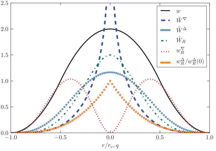
Figure 1: MPS weighting function and SPH equivalent kernels

As already pointed out in section 3.3 it is relevant that the gradient and Laplacian SPH derived kernels are different. It is interesting to note that the pressure effects, which are controlled by the gradient value, are modeled by using a singular kernel. The diffusive effects are on the other hand modeled by a regular kernel, with zero slope at the origin, which is necessary, as demonstrated by Violeau (2009) to obtain correct dissipation values.

It is pertinent to compare both kernels with the fourth order Wendland one (order here refers to the differentiability order at the boundary of the compact support), which has become very popular among SPH practitioners due to its outstanding anti-clumping properties (see e.g. (Dehnen and Aly, 2012; Robinson, 2009; Macià et al., 2011b; Valizadeh and Monaghan, 2012)). It can be appreciated in figure 1 that the Wendland kernel $\tilde{W}_{R}$ is not as spiky as $\tilde{W}_{\Delta}$ and not as flat as $\tilde{W}_{\nabla}$. Actually, it makes sense to obtain the equivalent MPS weighting function for this Wendland kernel specially for the gradient since singular kernels present problems when discretizing kernel integrals, as will be later discussed in this paper. In 1D the expression for the Wendland kernel is:

$$\tilde{W_{R}}(q)=\frac{3}{32}\left\{\begin{array}[]{cc}(2-2\,q)^{4}\,(1+4\,q),&0\leq q\leq 1,\\ 0,&1<q.\end{array}\right.$$ (47)

Equation (18) can now be used to obtain an MPS weighting function from an SPH kernel:

$$w(q):=-\frac{q}{d}\tilde{W}^{\prime}(q).$$ (48)

Notice that, from identity (94), with this definition of $w$ one has $A_{0}=1$.

For the Wendland kernel in 1D,

$$w_{R}^{\nabla}(q)=-q\tilde{W_{R}}^{\prime}(q)=30\left\{\begin{array}[]{cc}q^{2}-3\,q^{3}+3\,q^{4}-\,q^{5},&0\leq q\leq 1,\\ 0,&1<q.\end{array}\right.$$ (51)

Its graph can be seen in figure 1. One salient aspect to highlight is that it has a double hump and goes to zero at the origin, which makes it radically different from any of the MPS weighting functions documented in the literature (see e.g. Koshizuka and Oka (1996); Yoon et al. (1999b)). The reason for this is out of the scope of the present paper but may be related to the different nature of the pressure gradient model used in MPS (substraction of pressures in the interaction of a pair of particles) and the one used in SPH (addition of pressures in the interaction of a pair of particles).

The same can be done with the Laplacian equivalence (equation (29)) to obtain the MPS weighting function:

$$w(q):=-\frac{d}{q}\tilde{W}^{\prime}(q).$$ (52)

Notice that with this definition of $w$ one has $A_{2}=1$ from identity (94) in the appendix.

For the Wendland kernel in 1D:

$$w_{R}^{\Delta}(q)=-\frac{1}{q}\tilde{W_{R}}^{\prime}(q)=30\left\{\begin{array}[]{cc}1-3\,q+3\,q^{2}-q^{3},&0\leq q\leq 1,\\ 0,&1<q.\end{array}\right.$$ (55)

Its graph can be seen in figure 1. It has a non zero derivative at the origin so it essentially lays between the original weighting function $w$ from (Yoon et al., 1999b) and the singular weighting function used by e.g. Tsukamoto et al. (2011).

4 Boundary value problems

4.1 General

The fractional step method presented in section 2 requires solving a Poisson problem in each time-step. This Poisson problem is a partial differential equation boundary value problem defined in a compact domain $\Omega$ which involves the numerical approximation of the Laplacian operator for the left hand side. Dirichlet or mixed Neumann and Dirichlet boundary conditions (BCs) can be considered in order to obtain a unique solution.

In this section an MPS integral formulation of this boundary problem is analyzed in order to unveil inconsistencies present in the differential operators introduced in section 3 when applied to bounded domains. The problem is formulated in a general way as

$$\left\{\begin{array}[]{l}\Delta P(\mathbf{x})=f(\mathbf{x}),\qquad\mathbf{x}\in\Omega,\\ P(\mathbf{x})=g(\mathbf{x})\qquad\mathbf{x}\in\partial\Omega_{1},\\ \partial_{\mathbf{n}}P(\mathbf{x})=h(\mathbf{x})\qquad\mathbf{x}\in\partial\Omega_{2},\end{array}\right.$$ (59)

assuming that $\partial\Omega=\partial\Omega_{1}\cup\partial\Omega_{2}$ and that $\mathbf{n}$ is the exterior unitary normal to $\partial\Omega$.

The MPS Laplacian operator in its integral formulation (equation (27)) is now modified considering that the integrals over $\mathbb{R}^{d}$ are restricted to $\Omega$, which is where $P$ is defined:

$$\left\langle\Delta P\right\rangle\left(\mathbf{x}\right)\approx\frac{2d}{\left(r_{e}\right)^{d+2}A_{2}}\int_{\Omega}\left[P(\mathbf{x}^{\prime})-P(\mathbf{x})\right]w\left(\frac{\left|\mathbf{x}-\mathbf{x^{\prime}}\right|}{r_{e}}\right)d\mathbf{x^{\prime}}.$$ (60)

4.2 Zero Laplacian problem

A zero Laplacian problem ($f(\mathbf{x})=0$) for the pressure is relevant in this context since it is common that free-surface problems be driven by hydrostatic pressure dominated fields, which are linear, meaning that they have a zero Laplacian.

Writing the Laplacian in its integral formulation (equation (27)), it must hold for every $\mathbf{x}\in\Omega$ that:

$$\int_{\Omega}\left[P(\mathbf{x}^{\prime})-P(\mathbf{x})\right]w\left(\frac{\left|\mathbf{x}-\mathbf{x^{\prime}}\right|}{r_{e}}\right)d\mathbf{x^{\prime}}=0.$$ (61)

This is equivalent to:

$$P(\mathbf{x})\int_{\Omega}w\left(\frac{\left|\mathbf{x}-\mathbf{x^{\prime}}\right|}{r_{e}}\right)d\mathbf{x^{\prime}}=\int_{\Omega}P(\mathbf{x}^{\prime})\,w\left(\frac{\left|\mathbf{x}-\mathbf{x^{\prime}}\right|}{r_{e}}\right)d\mathbf{x^{\prime}}.$$ (62)

It turns out that the only solutions to equation (62) are the constant ones, as it is next shown.

Start noticing that since $P$ is a continuous function in $\overline{\Omega}$, it will reach a maximum in this domain. Let us denote by $\mathbf{x}^{*}$ the point at which $P$ takes its maximum. If $P$ is not identically constant, then this maximum must be strict. Hence, there exist points $\mathbf{x^{\prime}}$ such that $\left|\mathbf{x}^{*}-\mathbf{x^{\prime}}\right|<r_{e}$ and $P(\mathbf{x^{\prime}})<P(\mathbf{x^{*}})$. Since the weighting function $w$ is non-negative (see section 3.1), then one must have:

$$P(\mathbf{x}^{*})\int_{\Omega}w\left(\frac{\left|\mathbf{x}^{*}-\mathbf{x^{\prime}}\right|}{r_{e}}\right)d\mathbf{x^{\prime}}>\int_{\Omega}P(\mathbf{x}^{\prime})\,w\left(\frac{\left|\mathbf{x}^{*}-\mathbf{x^{\prime}}\right|}{r_{e}}\right)d\mathbf{x^{\prime}}.$$ (63)

This clearly contradicts equation (62) and therefore $P(\mathbf{x^{\prime}})=P(\mathbf{x^{*}}),\forall\mathbf{x^{\prime}}$.

This forces $P$ to be a constant function and thus the integral approximation to the boundary value problem (59) with $f(\mathbf{x})=0$ does not have a solution unless $g$ is constant. In such case, that constant is the only solution to the problem. A practical consequence of this to the analysis of the many-neighbor limit of the discrete MPS formulation will be discussed in section 5.5.1. It must be noticed that this regime is not reached in practical applications since the number of neighbors is limited by computational cost.

4.3 Constant sign source Poisson problem

We now consider a constant sign Laplacian problem for the pressure. This problem is relevant in this context since the divergence of the intermediate velocity field in equation (5) can maintain a constant sign for some intermediate flow fields. This can happen e.g. due to an expansion or contraction in free-surface flows, as in the standing wave case discussed in section 5.6.

Let us suppose that $f(\mathbf{x})$ in problem (59) has a positive constant sign ($f(\mathbf{x})\geq 0$ for every $\mathbf{x}\in\Omega$ with $f(\mathbf{x^{\prime}})>0$ for some $\mathbf{x^{\prime}}\in\Omega$). Writing the Laplacian in its integral formulation (equation (27)), one has that for every $\mathbf{x}\in\Omega$:

$$\int_{\Omega}\left[P(\mathbf{x}^{\prime})-P(\mathbf{x})\right]w\left(\frac{\left|\mathbf{x}-\mathbf{x^{\prime}}\right|}{r_{e}}\right)d\mathbf{x^{\prime}}=\frac{\left(r_{e}\right)^{d+2}A_{2}}{2d}f(\mathbf{x}),$$ (64)

which is equivalent to

$$P(\mathbf{x})\int_{\Omega}w\left(\frac{\left|\mathbf{x}-\mathbf{x^{\prime}}\right|}{r_{e}}\right)d\mathbf{x^{\prime}}=\int_{\Omega}P(\mathbf{x}^{\prime})\,w\left(\frac{\left|\mathbf{x}-\mathbf{x^{\prime}}\right|}{r_{e}}\right)d\mathbf{x^{\prime}}-\frac{\left(r_{e}\right)^{d+2}A_{2}}{2d}f(\mathbf{x}).$$ (65)

Since $P$ is a continuous function in $\Omega$, it will reach a maximum in this domain. Let us denote by $\mathbf{x}^{*}$ the point in which $P$ takes its maximum and assume it is strict for $\mathbf{x}$ close to $\mathbf{x}^{*}$ . Since the weighting function satisfies $w\geq 0$ (see section 3.1), then

$$P(\mathbf{x}^{*})\int_{\Omega}w\left(\frac{\left|\mathbf{x}^{*}-\mathbf{x^{\prime}}\right|}{r_{e}}\right)d\mathbf{x^{\prime}} >\int_{\Omega}P(\mathbf{x}^{\prime})\,w\left(\frac{\left|\mathbf{x}^{*}-\mathbf{x^{\prime}}\right|}{r_{e}}\right)d\mathbf{x^{\prime}}$$

$$\geq\int_{\Omega}P(\mathbf{x}^{\prime})\,w\left(\frac{\left|\mathbf{x}^{*}-\mathbf{x^{\prime}}\right|}{r_{e}}\right)d\mathbf{x^{\prime}}-\frac{\left(r_{e}\right)^{d+2}A_{2}}{2d}f(\mathbf{x}^{*}).$$ (66)

Therefore, since $f$ is non-negative, there is no $P$ verifying equation (65) at $\mathbf{x}^{*}$. Hence, the integral approximation to the boundary value problem (59) with $f(\mathbf{x})\geq 0$ does not have a solution. A similar reasoning can be done for a constant negative sign using the minimum of $P$ instead of its maximum to reach an identical conclusion. Similar considerations to those made in previous section regarding the practical implications of this issue apply here as well.

4.4 Consistent definition of MPS operators

4.4.1 General

The performance of the MPS Laplacian operator in its integral formulation has been shown to present significant problems for simple boundary value problems in compact domains. The impact of such problems at a discrete level will later be discussed with practical applications and will be addressed using the following corrected formulas for the MPS gradient, divergence and Laplacian, which involve the computation of boundary integrals using the related SPH kernels to each operator. The need for these boundary integrals arises from the fact that the integral domain is not $\mathbb{R}^{d}$ but $\Omega$.

The formulas are implemented in the MPS method by incorporating boundary integral terms (see (De Leffe et al., 2009; Colagrossi et al., 2009; Ferrand et al., 2012; Macià et al., 2012) for an analogous SPH treatment) and by using the SPH kernel - MPS weighting function equivalences presented in section 3.5.

The formulas to be introduced in sections 4.4.2-4.4.4 involve the following volume integrals of the equivalent SPH kernels (section 3.5):

$$\Gamma^{\nabla}\left(\mathbf{x}\right) =\int_{\Omega}W_{\nabla}\left(\mathbf{x}-\mathbf{x}^{\prime};r_{e}\right)d\mathbf{x}^{\prime},$$ (67)

$$\Gamma^{\Delta}\left(\mathbf{x}\right) =\int_{\Omega}W_{\Delta}\left(\mathbf{x}-\mathbf{x}^{\prime};r_{e}\right)d\mathbf{x}^{\prime}.$$ (68)

The reason for introducing these integrals will be explained in the following sections. Let us mention for the moment that equation (67) will play a role in our approximation to first order differential operators whereas equation (68) will be used in the approximation to the Laplacian.

4.4.2 Corrected MPS gradient

The proposed corrected formula for the MPS gradient is

$$\left\langle\nabla_{\mathbf{x}}\phi\right\rangle\left(\mathbf{x}\right) \approx\frac{d}{\left(r_{e}\right)^{d}A_{0}\,\Gamma^{\nabla}\left(\mathbf{x}\right)}\int_{\Omega}\frac{\phi(\mathbf{x^{\prime}})-\phi(\mathbf{x})}{{\left|\mathbf{x^{\prime}}-\mathbf{x}\right|^{2}}}\left(\mathbf{x^{\prime}}-\mathbf{x}\right)$$

$$w\left(\frac{\left|\mathbf{x}-\mathbf{x^{\prime}}\right|}{r_{e}}\right)d\mathbf{x^{\prime}}+\frac{1}{\Gamma^{\nabla}\left(\mathbf{x}\right)}\int_{\partial\Omega}\left(\phi(\mathbf{x^{\prime}})-\phi(\mathbf{x})\right)W_{\nabla}\left(\mathbf{x}-\mathbf{x}^{\prime};r_{e}\right)\,\mathbf{n}\,d\mathbf{x}^{\prime}.$$ (69)

The proposed correction is aimed at correcting the fact that weight function summations may not be complete close to the boundaries. For this reason the term $\Gamma^{\nabla}(\mathbf{x})$ is introduced in the denominator (it must be noticed that $\Gamma^{\nabla}(\mathbf{x})$ is equal to one when $\mathbf{x}$ is far from the boundary). Once this correction has been performed, the boundary term appears naturally as a result of applying the Green’s identity. It allows to perform accurate integrations close to the boundaries (it must be noticed that this boundary term vanishes identically when it is applied to a particle that is far from the boundary).

A nice feature of formula (4.4.2) is that it combines the use of the MPS weighting function $w$ and the equivalent SPH kernel $W_{\nabla}$. Its discrete formulation requires the discretization of the surface integral across $\partial\Omega$. Therefore it is necessary to explicitly define this surface. This is a tricky issue in fragmented flows but since MPS requires solving a boundary problem for the fractional step method, evaluating this boundary integral does not introduce additional difficulties. A simple alternative is to discretize $\partial\Omega$ in a series of surface elements of area $S_{j}$ each one with a particle at its centroid and with an exterior unitary normal $\mathbf{n}_{j}$. The integral in equation (4.4.2) can therefore be discretized as:

$$\left\langle\nabla\phi\right\rangle_{i} =\frac{d}{n_{0}\,\Gamma^{\nabla}_{i}}\sum_{j\neq i}\left[\frac{\phi_{j}-\phi_{i}}{{\left|\mathbf{x}_{j}-\mathbf{x}_{i}\right|^{2}}}\left(\mathbf{x}_{j}-\mathbf{x}_{i}\right)w\left(\frac{\left|\mathbf{x}_{j}-\mathbf{x}_{i}\right|}{r_{e}}\right)\right]$$

$$+\frac{1}{\Gamma^{\nabla}_{i}}\sum_{\mathbf{x}_{j}\in\partial\Omega}\left(\phi_{j}-\phi_{i}\right)W_{\nabla}\left(\mathbf{x}_{j}-\mathbf{x}_{i};r_{e}\right)\cdot\mathbf{n}_{j}\,S_{j}.$$ (70)

The kernel integrals (67) and (68) also have to be discretized to enter into this expression. A coherent MPS approach to these discretizations, taking into account equation (13) is

$$\Gamma^{\nabla}_{i} =\frac{A_{0}\,\left(r_{e}\right)^{d}}{n_{0}}\,\sum_{j\neq i}W_{\nabla}\left(\mathbf{x}_{j}-\mathbf{x}_{i};h\right)\text{,}$$ (71)

$$\Gamma^{\Delta}_{i} =\frac{A_{0}\,\left(r_{e}\right)^{d}}{n_{0}}\,\sum_{j}W_{\Delta}\left(\mathbf{x}_{j}-\mathbf{x}_{i};h\right).$$ (72)

4.4.3 Corrected MPS divergence

Formula (4.4.2) for the approximation of the partial derivatives is easily applied to the definition of a corrected formula for the MPS divergence:

$$\left\langle\nabla\cdot\mathbf{u}\right\rangle\left(\mathbf{x}\right) \approx\frac{d}{\left(r_{e}\right)^{d}A_{0}\,\Gamma^{\nabla}\left(\mathbf{x}\right)}\int_{\Omega}\frac{\left(\mathbf{u}^{\prime}-\mathbf{u}\right)\left(\mathbf{x^{\prime}}-\mathbf{x})\right)}{{\left|\mathbf{x^{\prime}}-\mathbf{x}\right|^{2}}}w\left(\frac{\left|\mathbf{x}-\mathbf{x^{\prime}}\right|}{r_{e}}\right)d\mathbf{x^{\prime}}$$

$$+\frac{1}{\Gamma^{\nabla}\left(\mathbf{x}\right)}\int_{\partial\Omega}\left(\mathbf{u}^{\prime}-\mathbf{u}\right)\cdot\mathbf{n}\,W_{\nabla}\left(\mathbf{x}-\mathbf{x}^{\prime};r_{e}\right)d\mathbf{x}^{\prime}.$$ (73)

This integral can be discretized analogously to the gradient one.

4.4.4 Corrected MPS Laplacian

The proposed corrected formula for the MPS Laplacian is

$$\left\langle\Delta\phi\right\rangle\left(\mathbf{x}\right) \approx\frac{2d}{\left(r_{e}\right)^{d+2}A_{2}\,\Gamma^{\Delta}\left(\mathbf{x}\right)}\int_{\Omega}\left[\phi(\mathbf{x}^{\prime})-\phi(\mathbf{x})\right]w\left(\frac{\left|\mathbf{x}-\mathbf{x^{\prime}}\right|}{r_{e}}\right)d\mathbf{x^{\prime}}$$

$$+\frac{2}{\Gamma^{\Delta}\left(\mathbf{x}\right)}\int_{\partial\Omega}\frac{\phi(\mathbf{x^{\prime}})-\phi(\mathbf{x})}{{\left|\mathbf{x^{\prime}}-\mathbf{x}\right|^{2}}}\left(\mathbf{x^{\prime}}-\mathbf{x}\right)W_{\Delta}\left(\mathbf{x}-\mathbf{x}^{\prime};r_{e}\right)\,\mathbf{n}\,d\mathbf{x}^{\prime}.$$ (74)

Introducing the boundary terms and the normalization factor $\Gamma^{\Delta}$ aims, analogously to the gradient and divergence approximations, at correcting the incompleteness of weight function summations and corresponding inaccuracies close to the boundaries (Macià et al., 2012).

The discrete version for this formula can be written as follows:

$$\langle\Delta\phi\rangle_{i} =\frac{2d}{\lambda n_{0}\,\Gamma^{\Delta}_{i}}\sum_{j\neq i}\left[\left(\phi_{j}-\phi_{i}\right)w\left(\frac{\left|\mathbf{x}_{j}-\mathbf{x}_{i}\right|}{r_{e}}\right)\right]$$

$$+\frac{2}{\Gamma^{\Delta}_{i}}\sum_{\mathbf{x}_{j}\in\partial\Omega}\frac{\phi_{j}-\phi_{i}}{{\left|\mathbf{x}_{j}-\mathbf{x}_{i}\right|^{2}}}\left(\mathbf{x}_{j}-\mathbf{x}_{i}\right)W_{\Delta}\left(\mathbf{x}_{j}-\mathbf{x}_{i};r_{e}\right)\cdot\mathbf{n}_{j}\,S_{j}.$$ (75)

In practice, the need for these corrections will be justified with some applications presented in section 5.

5 Applications

5.1 General

A series of analyses at the discrete level are now presented with the aim to show some practical consequences of the problems and proposed solutions documented in section 4.

The corrected formulas presented in section 4.4 incorporate the kernel integrals (67) and (68). These are evaluated using a sweep across the particles. The first discrete application will be to analyze the rate of convergence of those summations. We will focus on a one dimensional evenly-spaced setup, fixing the kernel/weighting function support radius and varying the resolution $\Delta x$ by increasing the number of particles.

Next, the accuracy and convergence of the MPS gradient and Laplacian operators will be compared with the proposed corrected versions. The divergence is not discussed in 1D since it coincides with the gradient.

A zero Laplacian boundary value problem in 1D with Dirichlet boundary conditions is then proposed. Dirichlet BCs are very important in MPS since in the Poisson equation for the pressure, the value of the pressure at the free surface particles is given.

A constant sign source term 1D Poisson problem with mixed Dirichlet and Neumann boundary conditions is then proposed. This is a relevant problem from a practical application point of view since solid boundary conditions for the pressure are modeled using a Neumann boundary condition.

Finally a two dimensional realistic flow consisting of the attenuation of a viscous standing wave is proposed. This flow has a Dirichlet BC on the free surface and a Neumann BC on the bottom of the tank; moreover, an analytic solution is available in the literature.

5.2 Kernel integrals

As discussed in section 4.4 and apparent from the new proposed formulae definitions presented in that section, the normalization factors $\Gamma^{\nabla}$ and $\Gamma^{\Delta}$ are a fundamental part of the new formulae. It is hence important to discuss how accurate the evaluation of these factors is, with the neighbors’ summations (71) and (72), before presenting comparisons between the classical formulae and the new proposed ones.

In this and the next three sections one dimensional problems will be considered. In all these examples the computational domain will be the closed interval $[0,1]$. The interaction range $r_{e}$ is set as 0.1. The limit $\delta x\rightarrow 0$, keeping $r_{e}$ fixed corresponds to the integral approximation discussed in the previous sections. This range of the parameters is not reached in practical applications due to computational cost but is the natural one to be considered in order to discuss consistency of the operators.

In figure 2 (left) it can be observed that for $\Gamma^{\nabla}$ the convergence to 1 is very slow, the patent reason for this being the singular nature of the kernel. The convergence to the exact values of the differential operators which involve this renormalization factor is therefore expected to be also slow. On the other hand, the convergence for the $\Gamma^{\Delta}$ factor is good (figure 2 right). For $r_{e}/\Delta x=2$ the exact value is obtained which is a convenient property to be later discussed.

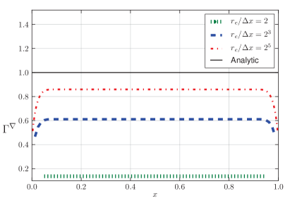
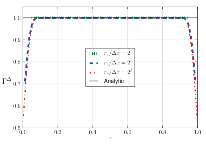
Figure 2: Kernel summations computed with the MPS gradient derived SPH kernel $\Gamma^{\nabla}$ (left) and with the MPS Laplacian derived SPH kernel $\Gamma^{\Delta}$ (right)

5.3 Gradient evaluation

Let us consider a linear field $P(x)=x$ for $x\in[0,1]$. In figure 3 (left) it can be appreciated that, keeping $r_{e}=0.1$ fixed, the gradient approximation provided by the classical MPS formula (14) converges to the exact value as $\Delta x$ goes to zero ($r_{e}/\Delta x\rightarrow\infty$) everywhere in the domain except at the boundaries, where the values are halved.

It can be appreciated that for $r_{e}/\Delta x=2$ the MPS evaluation of the gradient returns the exact solution. The solution for $r_{e}/\Delta x=2$ is exact because for evenly spaced particles, the MPS operator is equivalent to a second order centered finite difference scheme.

This is very promising but in practical applications the particles do not lie in a regular lattice. Let us slightly modify the particles positions by displacing them from the lattice with a random noise with maximum amplitude equal to $0.05\Delta x$. With this new configuration the results presented in figure 3 (right) are obtained. These results indicate that the effect of this low noise in lowering the accuracy of results is substantial.

It can be nonetheless appreciated that increasing the number of neighbors becomes a means to increase accuracy even for the disordered configuration. On one hand, one could think that reducing $r_{e}$ for a fixed number of neighbors could solve these problems but that may be in general not the case (Quinlan et al., 2006; Amicarelli et al., 2011).

On the other hand, increasing the number of neighbors allows to have more accurate approximations in the bulk of the domain but difficulties appear at the boundaries as can be seen in figures 3 (left) and (right). This lack of convergence to the exact solution close to the boundaries can be overcome by correcting the gradient formula (14) as indicated in section 4.4.2, using equation (4.4.2). Its one dimensional form is:

$$\left\langle P_{x}\right\rangle_{i} =\frac{1}{n_{0}\,\Gamma^{\nabla}_{i}}\sum_{j\neq i}\left[\frac{P_{j}-P_{i}}{{\left|x_{j}-x_{i}\right|^{2}}}\left(x_{j}-x_{i}\right)w\left(\frac{\left|x_{j}-x_{i}\right|}{r_{e}}\right)\right]$$

$$+\frac{1}{\Gamma^{\nabla}_{i}}\left[\left(P(1)-P_{i}\right)W_{\nabla}\left(1-x_{i};r_{e}\right)+\left(P_{i}-P(0)\right)W_{\nabla}\left(x_{i};r_{e}\right)\right].$$ (76)

Due to the singularity of the normalization factor for the gradient discussed in section 5.2, the convergence to the exact solutions for this formula is slow (figure 4 left) albeit clear, even close to the boundaries. An MPS weighting function which would give rise to an SPH regular kernel would be a good option to explore. The convergence is not affected by disordering the particles as can be appreciated in the left panel of figure 4.

Without entering into further consideration of disordered particle configurations, it seems clear that the ratio $\Delta x/r_{e}$ must be small (thus implying a significant number of neighboring particles) in order to obtain good interpolation properties for the first order differential operators (for both general configurations and areas close to the boundaries). In particular, this applies to the divergence operator, which is necessary when evaluating the source term of the Poisson equation (5) and the pressure gradient for the momentum equation (LABEL:Navier_Stokes_inc).

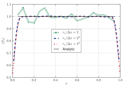
Figure 3: Gradient evaluation (section 5.3) with MPS Gradient (equation 14). Regular lattice (left), disordered lattice (right).

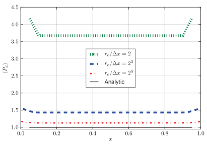
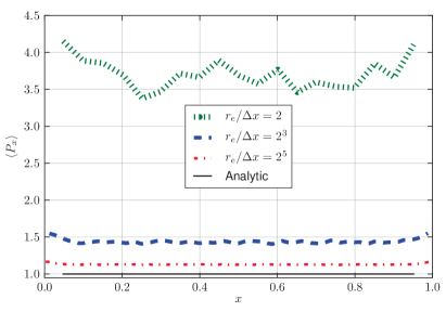
Figure 4: Gradient evaluation (section 5.3) with corrected MPS Gradient (4.4.2). Regular lattice (left), disordered lattice (right).

5.4 Laplacian evaluation

Let us now focus on a quadratic field $P(x)=x^{2}$ for $x\in[0,1]$. In figure 5 (left) it can be appreciated that, for $r_{e}=0.1$, the approximation to the Laplacian given by the classical MPS formulation (23) converges to the exact value as $\Delta x$ goes to zero everywhere in the interior of the domain. This is no longer the case on the boundary points where the operator becomes singular as $\Delta x/r_{e}$ goes to zero. Such singularity has been subject of investigation in the SPH context in e.g. (Colagrossi et al., 2011; Macià et al., 2011a). It can be overcome by correcting the formula as indicated in section 4.4.4 now using the equation which incorporates the boundary terms with the SPH kernel. Its one dimensional form is:

$$\left\langle P_{xx}\right\rangle_{i} =\frac{2}{\lambda\,n_{0}\,\Gamma^{\Delta}_{i}}\sum_{j\neq i}\left[\left(P_{j}-P_{i}\right)w\left(\frac{\left|x_{j}-x_{i}\right|}{r_{e}}\right)\right]$$

$$+\frac{2}{\Gamma^{\Delta}_{i}}\left[\frac{P(1)-P_{i}}{1-x_{i}}W_{\Delta}\left(1-x_{i};r_{e}\right)-\frac{P_{i}-P(0)}{x_{i}}W_{\Delta}\left(x_{i};r_{e}\right)\right].$$ (77)

The convergence is clear (figure 5 right) but quite slow due to the low order of the numerical derivatives involved in the boundary terms contributions of equation (4.4.4).

Coming back to figure 5, it can be appreciated that for $r_{e}/\Delta x=2$ the Laplacian is exact. This was also the case with the gradient evaluation of section 5.3, but as in that case, if the particles’ positions are displaced from the lattice with a random noise of just $0.05\Delta x$ maximum amplitude, figure 6 is obtained. This figure shows that the effect of this small disorder in the accuracy of results for small number of neighbors is substantial, and a similar discussion as that of section 5.3 applies here.

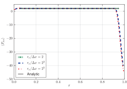
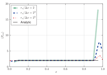
Figure 5: Laplacian evaluation (section 5.4) with a regular lattice: MPS Laplacian (23) (left), corrected MPS Laplacian (4.4.4) (right).

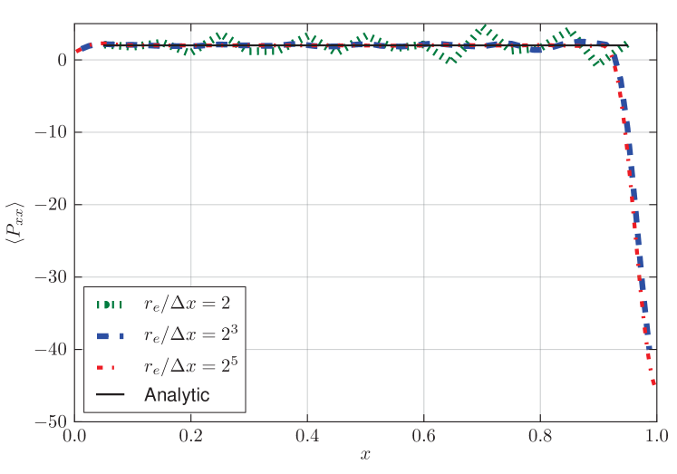
Figure 6: Laplacian evaluation (section 5.4), MPS Laplacian (23), noisy particle distribution.

5.5 Boundary value problems

5.5.1 1D zero Laplacian: Dirichlet boundary conditions

A 1D zero Laplacian problem whose exact solution is $P(x)=x$ is proposed:

$$\left\{\begin{array}[]{l}P^{\prime{}\prime{}}(x)=0,\qquad x\in[0,1],\\ P(0)=0,\\ P(1)=1.\end{array}\right.$$ (81)

The domain $[0,1]$ is discretized by fixing the cut-off radius $r_{e}$ and choosing the particle distance $\Delta x$ as a fraction of $r_{e}$. The MPS weighting function from (Yoon et al., 1999b) is used.

Equation (23) is used in the MPS method to compute the discrete Laplacian. Dirichlet boundary conditions are implemented in MPS (see i.e. (Koshizuka et al., 1998; Tsukamoto et al., 2011)) by identifying the particles defining the boundaries and then applying to those particles the corresponding value of the pressure. Their contribution to the Laplacian pass to the right hand side of the linear system that results from discretizing the boundary value problem.

Assuming $r_{e}=0.1$ and evenly spaced particles, the results for different values of the ratio $\Delta x/r_{e}$ are presented in figure 7. It is clear that, as we tend to the continuum ($\Delta x\rightarrow 0$), the solution does not converge to the analytical one $(p=x)$. It actually becomes discontinuous and tends, as a consequence of the lack of consistency of the integral operator discussed in section 4.2, to a constant function in the interior of the domain.

The solution for $r_{e}/\Delta x=2$ is exact because for evenly spaced particles, the MPS operator is equivalent to a second order centered finite difference scheme. Nonetheless, the need for a larger number of neighboring particles lies in the low interpolation properties of the gradient operator and Laplacian operator with disordered particles discussed in sections 5.3 and 5.4 respectively.

If the corrected Laplacian operator (4.4.4) is applied, the convergence to the exact solution is clear across the domain (figure 8 left and zoom in right).

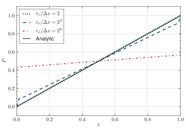
Figure 7: Solution of the boundary value problem (81), MPS Laplacian (23).

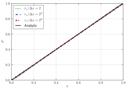
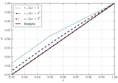
Figure 8: Solution of the boundary value problem (81), corrected MPS Laplacian (4.4.4) (right, zoom).

5.5.2 1D constant sign source: Dirichlet and Neumann boundary conditions

A 1D Poisson problem whose exact solution is $P(x)=x^{2}$ and which uses mixed Neumann and Dirichlet boundary conditions is proposed:

$$\left\{\begin{array}[]{l}P^{\prime{}\prime{}}(x)=2,\qquad x\in[0,1],\\ P^{\prime}(0)=0,\\ P(1)=1.\end{array}\right.$$ (85)

The domain $[0,1]$ is discretized by fixing the cut-off radius $r_{e}$ and choosing the particle distance $\Delta x$ as a fraction of $r_{e}$. The MPS weighting function from (Yoon et al., 1999b) is used.

Equation (23) is used in the MPS scheme to compute the discrete Laplacian. The Dirichlet boundary conditions implementation has been discussed in section 5.5.1. The Neumann boundary conditions are implemented by creating a set of dummy particles in the region with $x<0$. The pressure of all these dummy particles is taken equal to the pressure of the particle on the left boundary, $(x=0)$, which is in itself an unknown. The number of dummy particles is chosen in such a way that the number of neighbors remains constant (Tsukamoto et al., 2011). In figure 9 a sketch of the setup is presented.

Figure 9: Boundary value problem (85) discretization example sketch, with $r_{e}/\Delta x=2$.

Assuming $r_{e}=0.1$ the results for different values of the ratio $r_{e}/\Delta x$ are presented in figure 10. It is clear that as we tend to the continuum ($\Delta x\rightarrow 0$), the solution does not converge to the analytical one $(p(x)=x^{2})$. It does not either converge to a continuous solution of the integral formulation (64), becoming discontinuous at $(x=1)$.

As in the previous section, the solution for $r_{e}/\Delta x=2$ is exact for similar reasons.

If the corrected Laplacian operator (4.4.4) is applied, the exact solution is recovered for all the discretizations (figure 11 left and zoom in right).

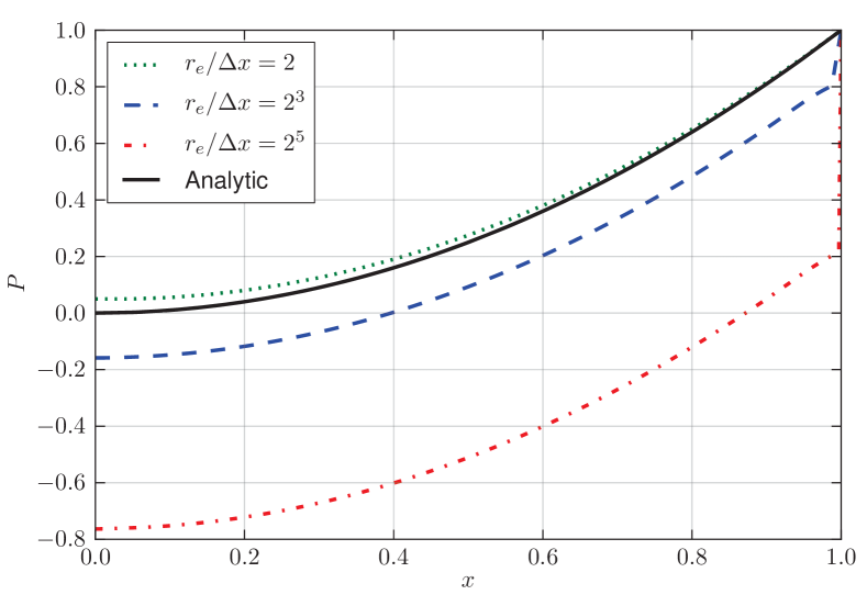
Figure 10: Solution of the boundary value problem (85), MPS Laplacian (23).

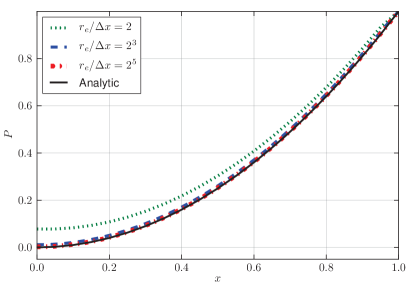
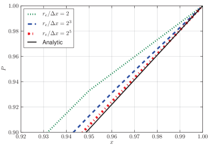
Figure 11: Solution of the boundary value problem (85), corrected MPS Laplacian (4.4.4) (right, zoom).

5.5.3 Symmetrized corrected Laplacian

The corrected Laplacian formula (4.4.4) is now modified symmetrizing the normalization factors so that the Poisson equation linear system becomes symmetric. This is very convenient from a computational point of view. Additionally this makes the formula conservative in terms of linear momentum. This is not so relevant in the MPS context since the gradient formula (the original and the corrected one) is not intrinsically conservative. Therefore, in the MPS version of equation (4) we have a conservative version of the discrete Laplacian and a non-conservative one for the pressure gradient. The proposed formula is

$$\langle\Delta\phi\rangle_{i} =\frac{2d}{\lambda n_{0}}\sum_{j\neq i}\left[\frac{1}{\Gamma^{\Delta}_{ij}}\left(\phi_{j}-\phi_{i}\right)w\left(\frac{\left|\mathbf{x}_{j}-\mathbf{x}_{i}\right|}{r_{e}}\right)\right]$$

$$+\sum_{\mathbf{x}_{j}\in\partial\Omega}\frac{2}{\Gamma^{\Delta}_{ij}}\frac{\phi_{j}-\phi_{i}}{{\left|\mathbf{x}_{j}-\mathbf{x}_{i}\right|^{2}}}\left(\mathbf{x}_{j}-\mathbf{x}_{i}\right)W_{\Delta}\left(\mathbf{x}_{j}-\mathbf{x}_{i};r_{e}\right)\cdot\mathbf{n}_{j}\,S_{j},$$ (86)

with

$$\Gamma^{\Delta}_{ij}=0.5\left(\Gamma^{\Delta}_{i}+\Gamma^{\Delta}_{j}\right).$$ (87)

As can be seen in figure 12, the effect of this symmetrization in the accuracy of the Poisson solver is negligible. For the sake of computational efficiency this will be the formula used for the free-surface flow discussed in the next section.

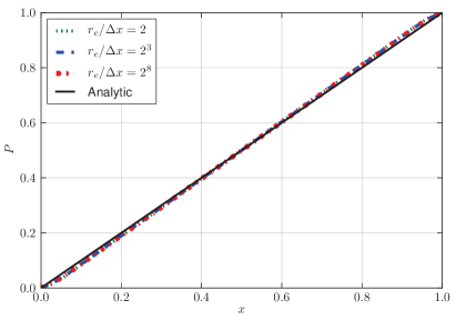
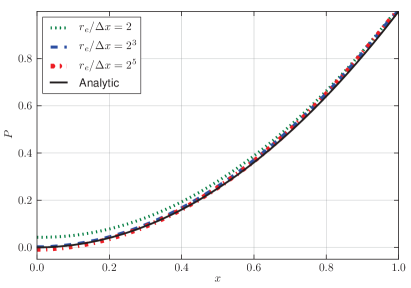
Figure 12: Solution of the boundary value problems (81) (left) and (85) (right) with corrected MPS symmetrized Laplacian (5.5.3).

5.6 Standing Wave

The objective of this paper has been to discuss the consistency of the MPS method, to establish its relationship with SPH, and to present alternative formulations for some of the operators. A full assessment of these new formulations when applied to complex 2D or 3D flows is not within the mentioned objectives and is left for future work. Nonetheless we think it is interesting to at least present an application of these operators to a realistic case considering the typical value for the MPS parameters used in the literature, specially the ratio $r_{e}/\Delta x$.

The evolution of a viscous standing wave has been chosen. This is a classical problem in the scientific literature for which an approximate analytical solution is available (Lighthill, 2001); it is of practical interest since it is related to the propagation of gravity waves. The standing wave flow has been widely studied in SPH (see e.g. Colagrossi et al. (2012, 2011); Antuono et al. (2011); Antuono and Colagrossi (2012)) and has been useful as well for validating mesh-based solvers (Carrica et al., 2007). Periodic boundary conditions have been imposed on the sides of the domain implying that the surface integrals of the corrected formulations are defined in straight segments making them easier to compute.

Finally, the particles are in a constant positive pressure state due to the presence of the hydrostatic pressure which prevents the onset of tensile instabilities. (Khayyer and Gotoh, 2011) performed an interesting validation study on MPS considering a set of interesting cases (rotating square, impinging jet, etc..) but not a standing wave one. They were interested in stability related problems, which is not within our goals. This is the primary reason for choosing a problem, the standing wave, for which numerical instabilities are not expected.

The chosen standing wave configuration consists in a rectangular tank with length $L$ and a water filling height of $H=L/2$. A sketch of this setup is displayed in figure 13. The wave length is $\lambda=L$, $k$ is the corresponding wave number (i.e. $k\,=\,2\pi/\lambda$), $A$ is the wave amplitude and $\epsilon$ denotes the ratio $2A/H$. The setup is the same used by Colagrossi et al. (2012).

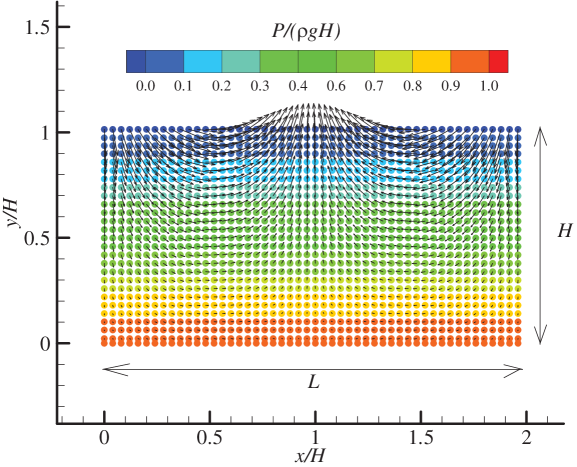
Figure 13: Notation and layout of the initial condition for the standing wave problem

For small-amplitude waves (i.e. small $\epsilon$), Potential Theory predicts the following approximate solution:

$$\begin{array}[]{ll}\displaystyle{\varphi}(x,y,t)\,=\,\varphi_{0}(x,y)\,\cos(\omega\,t)\,;\,\quad\varphi_{0}(x,y)\,=\,-\,\epsilon\,\frac{H\,g}{2\,\omega}\,\frac{\cosh[k(y+H)]}{\cosh(kH)}\,\cos(k\,x).\end{array}$$ (89)

Here, the circular frequency $\omega$ is given by the dispersion relation of gravity waves, that is, $\omega^{2}\,=\,g\,k\,\tanh(k\,H)$ where $g$ is the acceleration of gravity. At time $t=0$ the free surface is horizontal while the initial fluid velocity is given by $\nabla\varphi_{0}$.

Potential Theory predicts that the total energy of the standing wave is conserved during the evolution. However, if the fluid is viscous and the dissipation due to the solid boundary layers is neglected, it is possible to obtain an approximate analytical solution that gives the decay of the kinetic energy (see (Lighthill, 2001)). This is

$$\mathcal{E}_{K}(t)\,=\,\epsilon^{2}\,g\,\frac{\lambda\,H^{2}}{32}\,e^{-4\,\nu\,k^{2}\,t}\,\big{[}\,1\,+\,\cos(2\,\omega\,t)\,\big{]}.$$ (90)

The coefficient of the exponential ($4\,\nu\,k^{2}$), which governs the kinetic attenuation rate, depends on the wave number and on the kinematic viscosity $\nu=\mu/\rho$. The MPS simulations have been implemented by using a free-slip condition for the velocity and a Neumann condition for the pressure along the bottom boundary of the tank, and periodic BCs on the lateral sides. This is in accordance with the hypothesis made by Lighthill (2001) in which only internal and free surface viscous boundary layer dissipation sources are considered.

A set of two simulations with parameter values $g=1$, $L=2$, $\epsilon=0.1$ and $H/\Delta x=50,100$, using both the classical and corrected formulations have been carried out. The Reynolds number is $Re=H\sqrt{gH}/\nu=250$, high enough for the Lighthill approximation to be reasonably accurate. A value of $r_{e}/\Delta x=4$ for the Laplacian and $r_{e}/\Delta x=2$ for the gradient are taken, which are common for MPS practitioners (see e.g. Yoon et al. (1999b); Tsukamoto et al. (2011)).

In figure 14 the decay of the kinetic energy is displayed using a classical MPS scheme and the proposed corrected formulas discussed in section 4.4. The corrected approach performs better when compared to the analytical solution with significant over-damping observed in the classical approach. A plot of the velocity field modulus after half an oscillation cycle, normalized with the maximum initial velocity, is provided in figure 15. The graphs show the extra damping occurring in the classical approach simulations, made noticeable by the differences in the velocity modulus in the area close to the free surface. This evidence is not enough to proclaim any general conclusion although the results are promising. Further investigation is left for future work.

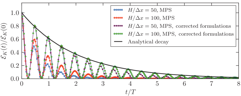
Figure 14: Standing wave kinetic energy time evolution

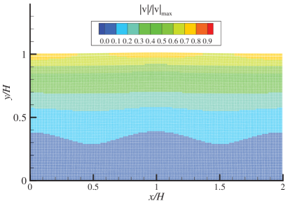
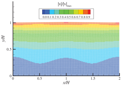
Figure 15: Velocity field modulus at the second kinetic energy peak, $t/T\approx 0.5$, uncorrected formulation (left), corrected (right).

6 Conclusions

The consistency of the moving particle semi-implicit (MPS) method in reproducing the gradient, divergence and Laplacian differential operators has been discussed in the present paper. It has been shown that the operators are consistent by performing an analogy with the SPH formulations. The equivalence between the MPS weighting function and the SPH kernel has been established. It has been shown that this equivalence differs for the first order and second order differential operators leading to different equivalent SPH kernels formulations. It has been shown that for each MPS weighting function it is possible to find two SPH kernels, one which allows the computation of the MPS gradient and a different one for the Laplacian. It has been shown that the converse also holds; from an SPH kernel two MPS weighting functions can be obtained, one using the gradient equivalence and another, the Laplacian equivalence. To summarize, we show that SPH and MPS are closely related.

SPH started earlier in the seventies and was applied in the early nineties to free-surface flows using an explicit approach with a weakly compressible fluid model to numerically simulate liquid behavior. Later in the mid nineties, the MPS method appeared imposing incompressibility with a projection scheme. In the late nineties a similar approach was followed to obtain the first incompressible SPH model. From then on, they have run parallel, approaching a wide range of problems. The connections amongst them have been clearly established in the present paper through the comparison of the differential operators and the convolution functions. We believe this can be useful in order to establish a common framework that can help the progress of both methods.

The application of the MPS scheme in solving the Navier-Stokes equations, using a fractional step approach, has been treated. Some inconsistency problems when solving the Poisson equation in the fractional step method have been unveiled. It has been shown that in general, such an equation does not have a solution when using the MPS integral formulation. Due to the equivalences shown, the same inconsistency problems occur with the incompressible SPH method.

A corrected formulation of the operators has been proposed involving the use of boundary integrals. Applications to one dimensional boundary value Dirichlet and mixed Neumann-Dirichlet problems have been presented. These applications show that the use of the corrected formulations is crucial in order to obtain a convergence to the exact results in all these problems.

Although in this work we have not focused on validation of practical fluid mechanics problems, a complex free-surface flow application, namely the evolution of a viscous standing wave has been briefly discussed. We have shown that the corrected formulations improve the accuracy of the results under the analyzed conditions.

As a final remark, and after showing the equivalence of MPS and SPH methods, we would like to stress that, although being crucial in guaranteeing convergence to the exact solution, consistency is not the only factor to take into account in order to have a reliable numerical method. Stability, conservation properties and computational feasibility are equally important. Translating all the existing results available in the MPS literature to SPH and viceversa is left, amongst other things, as future work.

Appendix A SPH approximation of differential operators

A.1 General

Smoothed Particle Hydrodynamics (SPH) is a numerical method used among many other applications to solve the Navier-Stokes equations. It has very attractive features for certain types of flows, namely that it is mesh-free, its Lagrangian character and its conservation properties. SPH has been used in a wide range of contexts, including Astrophysics (Benz, 1988), Magnetohydrodynamics (Price, 2012), free surface flows (Monaghan, 1994; Gomez-Gesteira et al., 2010), Coastal Engineering applications (Dalrymple and Rogers, 2006) and even Solid Mechanics (Libersky et al., 1993). A comprehensive recent review of the method can be found in (Violeau, 2012). In SPH both a weakly compressible approach in order to impose incompressibility (Monaghan, 2005) and a pure incompressible one (Cummins and Rudman, 1999; Lee et al., 2008) similar to MPS have coexisted through the years.

In this appendix, the continuous version of the SPH modeling of the gradient and Laplacian differential operators together with some related consistency statements are introduced; they are useful in describing the equivalences with the MPS method discussed in the bulk of the paper.

A.2 Kernel

Let $W\left(\mathbf{x};h\right)$ be the function of $\mathbf{x}\in\mathbb{R}^{d}$ depending on $h>0$ defined by

$$W\left(\mathbf{x};h\right)=\frac{1}{h^{d}}\tilde{W}\left(\left|\frac{\mathbf{x}}{h}\right|\right)\text{,}$$ (91)

where $\tilde{W}:\mathbb{R\rightarrow R}$ is a nonnegative differentiable function such that:

$$\int_{\mathbb{R}^{d}}\tilde{W}\left(\left|\mathbf{x}\right|\right)d\mathbf{x}=1.$$ (92)

When $d>1$

$$\int_{\mathbb{R}^{d}}\tilde{W}\left(\left|\mathbf{x}\right|\right)d\mathbf{x}=\omega_{d}\int_{0}^{\infty}\tilde{W}\left(r\right)r^{d-1}dr,$$ (93)

the constant $\omega_{d}$ being the volume of the unit sphere in $\mathbb{R}^{d}$.

An important result used in the calculations documented in the paper in order to establish the relationships existing between the SPH kernel and the MPS weighting functions is the following:

$$\int_{\mathbb{R}^{d}}\tilde{W}(\left|\mathbf{x}\right|)d\mathbf{x}=-\frac{1}{d}\int_{\mathbb{R}^{d}}\left|\mathbf{x}\right|\tilde{W}^{\prime}(\left|\mathbf{x}\right|)d\mathbf{x}.$$ (94)

This relationship is a direct consequence of the following identities obtained through integration by parts

$$-\int_{\mathbb{R}^{d}}\frac{x_{k}^{2}}{\left|\mathbf{x}\right|}\tilde{W}^{\prime}(\left|\mathbf{x}\right|)d\mathbf{x}=-\int_{\mathbb{R}^{d}}x_{k}\partial_{x_{k}}\tilde{W}(\left|\mathbf{x}\right|)d\mathbf{x}=\int_{\mathbb{R}^{d}}\tilde{W}(\left|\mathbf{x}\right|)d\mathbf{x},$$

after summing over $k$.

A.3 Continuous SPH approximation

The SPH approximation with respect to the kernel $W$ of a function $u\left(\mathbf{x}\right)$ on $\mathbb{R}^{d}$ taking real values is defined as:

$$\left\langle u\right\rangle\left(\mathbf{x}\right):={\displaystyle\int_{\mathbb{R}^{d}}}u\left(\mathbf{x}^{\prime}\right)W\left(\mathbf{x-x}^{\prime};h\right)d\mathbf{x}^{\prime}$$ (95)

A.4 Derivatives

The SPH approximation of the partial derivative $\partial_{x_{k}}u$ is set to be:

$$\left\langle\partial_{x_{k}}u\right\rangle\left(\mathbf{x}\right):=\int_{\mathbb{R}^{d}}u\left(\mathbf{x}^{\prime}\right)\partial_{x_{k}}W\left(\mathbf{x-x}^{\prime};h\right)d\mathbf{x}^{\prime}.$$ (96)

Note that $\left\langle\partial_{x_{k}}u\right\rangle$ coincides with $\partial_{x_{k}}\left\langle u\right\rangle$. In addition, since

$$\nabla_{\mathbf{x}}W\left(\mathbf{x;}h\right)=\frac{1}{h^{d+1}}\tilde{W}^{\prime}\left(\frac{\left|\mathbf{\mathbf{x}}\right|}{h}\right)\frac{\mathbf{x}}{\left|\mathbf{x}\right|},$$

we can write

$$\left\langle\partial_{x_{k}}u\right\rangle\left(\mathbf{x}\right)=\frac{1}{h^{d+1}}\int_{\mathbb{R}^{d}}u\left(\mathbf{x}^{\prime}\right)\frac{x_{k}-x_{k}^{{}^{\prime}}}{\left|\mathbf{x}-\mathbf{x}^{\prime}\right|}\tilde{W}^{\prime}\left(\frac{\left|\mathbf{\mathbf{x-x}}^{\prime}\right|}{h}\right)d\mathbf{x}^{\prime}$$ (97)

The previous expression can be anti-symmetrized so that, at the discrete level, the derivative of a constant function is identically zero. Note that:

$$\int_{\mathbb{R}^{d}}\frac{{x_{k}-x_{k}^{\prime}}}{\left|\mathbf{x}-\mathbf{x}^{\prime}\right|}\tilde{W}^{\prime}\left(\frac{\left|\mathbf{\mathbf{x-x}}^{\prime}\right|}{h}\right)d\mathbf{x}^{\prime}=0.$$

Therefore (97) is also equal to:

$$\left\langle\partial_{x_{k}}u\right\rangle\left(\mathbf{x}\right)=\frac{1}{h^{d+1}}\int_{\mathbb{R}^{d}}\frac{u\left(\mathbf{x}^{\prime}\right)-u\left(\mathbf{x}\right)}{\left|\mathbf{x}-\mathbf{x}^{\prime}\right|}\left({x_{k}-x_{k}^{\prime}}\right)\tilde{W}^{\prime}\left(\frac{\left|\mathbf{\mathbf{x-x}}^{\prime}\right|}{h}\right)d\mathbf{x}^{\prime}.$$ (98)

Nonetheless, the discrete version of this formula does not conserve linear momentum when used to evaluate the pressure gradient and it is generally replaced by a similar one which is instead symmetric (see (Monaghan, 2005) for a specific discussion on this topic).

The divergence operator can be written as:

$$\left\langle\nabla\cdot\mathbf{u}\right\rangle\left(\mathbf{x}\right)=\frac{1}{h^{d+1}}\int_{\mathbb{R}^{d}}\frac{\left(\mathbf{u}\left(\mathbf{x}^{\prime}\right)-\mathbf{u}\left(\mathbf{x}\right)\right)\cdot\left(\mathbf{x}-\mathbf{x^{\prime}}\right)}{\left|\mathbf{x}-\mathbf{x}^{\prime}\right|}\tilde{W}^{\prime}\left(\frac{\left|\mathbf{\mathbf{x-x}}^{\prime}\right|}{h}\right)d\mathbf{x}^{\prime},$$ (99)

which is identically zero for constant fields at the discrete level.

A.5 The Laplacian

We will consider the following SPH approximation of the Laplacian of a function $u\left(\mathbf{x}\right)$ due to Morris et al. (1997) whose consistency was demonstrated by Español and Revenga (2003).

$$\left\langle\Delta u\right\rangle\left(\mathbf{x}\right):=2\int_{\mathbb{R}^{d}}\frac{\left(\mathbf{x}^{\prime}-\mathbf{x}\right)\cdot\nabla_{\mathbf{x}}W\left(\mathbf{x}^{\prime}-\mathbf{x;}h\right)}{\left|\mathbf{x}^{\prime}-\mathbf{x}\right|^{2}}\left[u\left(\mathbf{x}^{\prime}\right)-u\left(\mathbf{x}\right)\right]d\mathbf{x}^{\prime}.$$ (100)

In order to compare this expression to the MPS approximation of the Laplacian, it is useful to rewrite (100)as:

$$\left\langle\Delta u\right\rangle\left(\mathbf{x}\right)=-\frac{2}{h^{d+1}}\int_{\mathbb{R}^{d}}\frac{u\left(\mathbf{x}^{\prime}\right)-u\left(\mathbf{x}\right)}{\left|\mathbf{x}^{\prime}-\mathbf{x}\right|}\tilde{W}^{\prime}\left(\frac{\left|\mathbf{\mathbf{x}^{\prime}-\mathbf{x}}\right|}{h}\right)d\mathbf{x}^{\prime}.$$ (101)

A.6 Consistency

The reader is referred to (Macià et al., 2011a) for details on consistency results of SPH approximation to differential operators. A summary is provided here. For a general twice differentiable function $u$ the following holds:

$$\left\langle u\right\rangle=u+\mathcal{O}\left(h^{2}\right),$$

$$\left\langle\nabla_{\mathbf{x}}u\right\rangle=\nabla_{\mathbf{x}}u+\mathcal{O}\left(h^{2}\right),\qquad\langle\nabla\cdot\mathbf{u}\rangle=\nabla\cdot\mathbf{u}+\mathcal{O}\left(h^{2}\right),\qquad\left\langle\Delta u\right\rangle=\Delta u+\mathcal{O}\left(h^{2}\right).$$

References

-
Amicarelli et al. (2011)
Amicarelli, A., Marongiu, J.-C., Leboeuf, F., Leduc, J., Caro, J., 2011. SPH
truncation error in estimating a 3D function. Computers & Fluids 44 (1),
279 – 296.
URL http://www.sciencedirect.com/science/article/B6V26-52079TP-1/2/28aecd9efa85d26137ba55bcaa45daa4 -
Antuono and Colagrossi (2012)
Antuono, M., Colagrossi, A., 2012. The damping of viscous gravity waves. Wave
Motion (0), –.
URL http://www.sciencedirect.com/science/article/pii/S0165212512001060 -
Antuono et al. (2011)
Antuono, M., Colagrossi, A., Marrone, S., Lugni, C., 2011. Propagation of
gravity waves through an SPH scheme with numerical diffusive terms.
Computer Physics Communications 182 (4), 866 – 877.
URL http://www.sciencedirect.com/science/article/B6TJ5-51PRYCS-1/2/b69f4a14370f08b80c197c90035b226a - Benz (1988) Benz, W., 1988. Applications of smoothed particle hydrodynamics (sph) to astrophysical problems. Computer Physics Communications 48, 97–105.
-
Carrica et al. (2007)
Carrica, P. M., Wilson, R. V., Stern, F., 2007. An unsteady single-phase level
set method for viscous free surface flows. International Journal for
Numerical Methods in Fluids 53 (2), 229–256.
URL http://dx.doi.org/10.1002/fld.1279 -
Chorin (1968)
Chorin, A. J., Oct. 1968. Numerical Solution of the Navier-Stokes Equations.
Mathematics of Computation 22 (104), 745–762.
URL http://dx.doi.org/10.2307/2004575 - Colagrossi et al. (2011) Colagrossi, A., Antuono, M., Souto-Iglesias, A., Le Touzé, D., 2011. Theoretical analysis and numerical verification of the consistency of viscous smoothed-particle-hydrodynamics formulations in simulating free-surface flows. Physical Review E 84, 26705+.
- Colagrossi et al. (2009) Colagrossi, A., Antuono, M., Touzé, D. L., 2009. Theoretical considerations on the free-surface role in the Smoothed-particle-hydrodynamics model. Physical Review E (Statistical, Nonlinear, and Soft Matter Physics) 79 (5), 056701.
- Colagrossi et al. (2012) Colagrossi, A., Souto-Iglesias, A., Antuono, M., Marrone, S., 2012. SPH modeling of dissipation mechanisms in gravity waves. (submitted for publication).
- Cummins and Rudman (1999) Cummins, S., Rudman, M., July 1999. An SPH projection method. J. Comp. Phys. 152 (2), 584–607.
- Dalrymple and Rogers (2006) Dalrymple, R., Rogers, B., 2006. Numerical modeling of water waves with the sph method. Coastal Engineering 53 (2-3), 141–147.
- De Leffe et al. (2009) De Leffe, M., Le Touzé, D., Alessandrini, B., May 2009. Normal flux method at the boundary for SPH. In: SPHERIC. pp. 149–156.
-
Dehnen and Aly (2012)
Dehnen, W., Aly, H., 2012. Improving convergence in smoothed particle
hydrodynamics simulations without pairing instability. Monthly Notices of the
Royal Astronomical Society 425 (2), 1068–1082.
URL http://dx.doi.org/10.1111/j.1365-2966.2012.21439.x - Español and Revenga (2003) Español, P., Revenga, M., Feb 2003. Smoothed dissipative particle dynamics. Phys. Rev. E 67 (2), 026705.
-
Ferrand et al. (2012)
Ferrand, M., Laurence, D., Rogers, B., Violeau, D., Kassiotis, C., 2012.
Unified semi-analytical wall boundary conditions for inviscid, laminar or
turbulent flows in the meshless SPH method. International Journal for
Numerical Methods in Fluids, n/a–n/a.
URL http://dx.doi.org/10.1002/fld.3666 -
Gomez-Gesteira et al. (2010)
Gomez-Gesteira, M., Rogers, B. D., Dalrymple, R. A., Crespo, A. J. C., 2010.
State-of-the-art of classical SPH for free-surface flows. Journal of
Hydraulic Research 48 (S1), 6–27.
URL http://dx.doi.org/10.1080/00221686.2010.9641242 -
Khayyer and Gotoh (2009a)
Khayyer, A., Gotoh, H., 2009a. Modified moving particle
semi-implicit methods for the prediction of 2d wave impact pressure. Coastal
Engineering 56 (4), 419 – 440.
URL http://www.sciencedirect.com/science/article/pii/S0378383908001646 - Khayyer and Gotoh (2009b) Khayyer, A., Gotoh, H., December 2009b. Wave impact pressure calculations by improved SPH methods. International Journal of Offshore and Polar Engineering 19 (4), 300–307.
-
Khayyer and Gotoh (2010)
Khayyer, A., Gotoh, H., 2010. A higher order laplacian model for enhancement
and stabilization of pressure calculation by the mps method. Applied Ocean
Research 32 (1), 124 – 131.
URL http://www.sciencedirect.com/science/article/pii/S0141118710000027 -
Khayyer and Gotoh (2011)
Khayyer, A., Gotoh, H., 2011. Enhancement of stability and accuracy of the
moving particle semi-implicit method. Journal of Computational Physics
230 (8), 3093 – 3118.
URL http://www.sciencedirect.com/science/article/pii/S0021999111000271 -
Khayyer and Gotoh (2012)
Khayyer, A., Gotoh, H., 2012. A 3d higher order laplacian model for enhancement
and stabilization of pressure calculation in 3d mps-based simulations.
Applied Ocean Research 37 (0), 120 – 126.
URL http://www.sciencedirect.com/science/article/pii/S0141118712000399 - Koshizuka et al. (1998) Koshizuka, S., Nobe, A., Oka, Y., 1998. Numerical analysis of breaking waves using the moving particle semi-implicit method. International Journal for Numerical Methods in Fluids 26 (7), 751–769.
- Koshizuka and Oka (1996) Koshizuka, S., Oka, Y., 1996. Moving-particle semi-implicit method for fragmentation of incompressible fluid. Nuclear Science and Engineering 123 (3), 421–434.
- Koshizuka et al. (1995) Koshizuka, S., Oka, Y., Tamako, H., 1995. A particle method for calculating splashing of incompressible viscous fluid. In: International Conference, Mathematics and Computations, Reactor Physics, and Environmental Analyses. Vol. 2. pp. 1514–1521.
- Laibe and Price (2012a) Laibe, G., Price, D. J., Mar. 2012a. Dusty gas with smoothed particle hydrodynamics - I. Algorithm and test suite. Monthly Notices of the RAS 420, 2345–2364.
- Laibe and Price (2012b) Laibe, G., Price, D. J., Mar. 2012b. Dusty gas with smoothed particle hydrodynamics - II. Implicit timestepping and astrophysical drag regimes. Monthly Notices of the RAS 420, 2365–2376.
- Lee et al. (2008) Lee, E. S., Moulinec, C., Xu, R., Violeau, D., Laurence, D., Stansby, P., 9/10 2008. Comparisons of weakly compressible and truly incompressible algorithms for the SPH mesh free particle method. Journal of Computational Physics 227 (18), 8417–8436.
- Libersky et al. (1993) Libersky, L., Petschek, A., Carney, T., Hipp, J., Allahdadi, F., 1993. High strain lagrangian hydrodynamics a three-dimensional sph code for dynamic material response. J. Comp. Phys. 109 (1), 67–75.
- Lighthill (2001) Lighthill, J., 2001. Waves in fluids. Cambridge University Press.
-
Macià et al. (2011a)
Macià, F., Antuono, M., González, L. M., Colagrossi, A.,
2011a. Theoretical analysis of the no-slip boundary condition
enforcement in SPH methods. Progress of Theoretical Physics 125 (6),
1091–1121.
URL http://ptp.ipap.jp/link?PTP/125/1091/ - Macià et al. (2011b) Macià, F., Colagrossi, A., Antuono, M., Souto-Iglesias, A., 2011b. Benefits of using a Wendland kernel for free-surface flows. In: 6th ERCOFTAC SPHERIC workshop on SPH applications. Hamburg University of Technology, pp. 30–37.
-
Macià et al. (2012)
Macià, F., González, L. M., Cercos-Pita, J. L., Souto-Iglesias, A.,
Sep. 2012. A boundary integral SPH formulation. Consistency and
applications to ISPH and WCSPH. Progress of Theoretical Physics 128 (3).
URL # - Monaghan (1994) Monaghan, J., 1994. Simulating free surface flows with SPH. J. Comp. Phys. 110 (2), 39–406.
-
Monaghan (2012)
Monaghan, J., 2012. Smoothed particle hydrodynamics and its diverse
applications. Annual Review of Fluid Mechanics 44 (1), 323–346.
URL http://www.annualreviews.org/doi/abs/10.1146/annurev-fluid-120710-101220 - Monaghan (2005) Monaghan, J. J., 2005. Smoothed particle hydrodynamics. Reports on Progress in Physics 68, 1703–1759.
- Morris et al. (1997) Morris, J. P., Fox, P. J., Zhu, Y., 1997. Modeling low Reynolds number incompressible flows using SPH. Journal of Computational Physics 136, 214–226.
- Naito and Sueyoshi (2001) Naito, S., Sueyoshi, M., Sept. 2001. A numerical analysis of violent free surface flow on flooded car deck using particle method. In: 5th International Workshop Stability and Operational Safety of Ships. Trieste.
-
Price (2012)
Price, D. J., 2012. Smoothed particle hydrodynamics and magnetohydrodynamics.
Journal of Computational Physics 231 (3), 759 – 794.
URL http://www.sciencedirect.com/science/article/pii/S0021999110006753 -
Quinlan et al. (2006)
Quinlan, N. J., Lastiwka, M., Basa, M., 2006. Truncation error in mesh-free
particle methods. International Journal for Numerical Methods in Engineering
66 (13), 2064–2085.
URL http://dx.doi.org/10.1002/nme.1617 - Robinson (2009) Robinson, M., 2009. Turbulence and Viscous Mixing using Smoothed Particle Hydrodynamics. Ph.D. thesis, Department of Mathematical Science, Monash University.
- Sueyoshi and Naito (2003) Sueyoshi, M., Naito, S., Sept. 2003. A numerical study of violent free surface problems with particle method for marine engineering. In: 8th International Conference on Numerical Ship Hydrodynamics, Busan(Korea). pp. 330–339.
-
Tanaka and Masunaga (2010)
Tanaka, M., Masunaga, T., 2010. Stabilization and smoothing of pressure in mps
method by quasi-compressibility. Journal of Computational Physics 229 (11),
4279 – 4290.
URL http://www.sciencedirect.com/science/article/pii/S0021999110000847 -
Tsukamoto et al. (2011)
Tsukamoto, M. M., Cheng, L.-Y., Nishimoto, K., 2011. Analytical and numerical
study of the effects of an elastically-linked body on sloshing. Computers &
Fluids 49 (1), 1 – 21.
URL http://www.sciencedirect.com/science/article/pii/S0045793011001423 -
Valizadeh and Monaghan (2012)
Valizadeh, A., Monaghan, J. J., 2012. Smoothed particle hydrodynamics
simulations of turbulence in fixed and rotating boxes in two dimensions with
no-slip boundaries. Physics of Fluids 24 (3), 035107.
URL http://link.aip.org/link/?PHF/24/035107/1 -
Violeau (2009)
Violeau, D., Sep 2009. Dissipative forces for lagrangian models in
computational fluid dynamics and application to smoothed-particle
hydrodynamics. Phys. Rev. E 80, 036705.
URL http://link.aps.org/doi/10.1103/PhysRevE.80.036705 - Violeau (2012) Violeau, D., 2012. Fluid Mechanics and the SPH Method. Oxford University Press.
- Yoon et al. (1999a) Yoon, H.-Y., Koshizuka, S., Oka, Y., 1999a. A mesh-free numerical method for direct simulation of gas-liquid phase interface. Nuclear-Science-and-Engineering 133 (2), 192–200.
- Yoon et al. (1999b) Yoon, H.-Y., Koshizuka, S., Oka, Y., 1999b. A particle-gridless hybrid method for incompressible flows. International Journal for Numerical Methods in Fluids 30 (4), 407–424.