Evolution of the tangent vectors and localization
of the stable and unstable manifolds of hyperbolic orbits
by Fast Lyapunov Indicators

Abstract

The Fast Lyapunov Indicators are functions defined on the tangent fiber of the phase–space of a discrete (or continuous) dynamical system, by using a finite number of iterations of the dynamics. In the last decade, they have been largely used in numerical computations to localize the resonances in the phase–space and, more recently, also the stable and unstable manifolds of normally hyperbolic invariant manifolds. In this paper, we provide an analytic description of the growth of tangent vectors for orbits with initial conditions which are close to the stable-unstable manifolds of a hyperbolic saddle point of an area–preserving map. The representation explains why the Fast Lyapunov Indicator detects the stable-unstable manifolds of all fixed points which satisfy a certain condition. If the condition is not satisfied, a suitably modified Fast Lyapunov Indicator can be still used to detect the stable-unstable manifolds. The new method allows for a detection of the manifolds with a number of precision digits which increases linearly with respect to the integration time. We illustrate the method on the critical problem of detection of the so–called tube manifolds of the Lyapunov orbits of $L_{1},L_{2}$ in the circular restricted three–body problem.

1 Introduction

Since the first detection of chaotic motions in 1964 (Henon–Heiles [17]), several indicators have been largely used to characterize the different dynamics of dynamical systems. Many dynamical indicators, such as the Lyapunov characteristic exponents and the more recently introduced finite–time chaos indicators (such as the Finite Time Lyapunov Exponent–FTLE [31], Fast Lyapunov Indicator–FLI [7], Mean Exponential Growth of Nearby Orbits–MEGNO [4]), are defined by the local divergence of nearby initial conditions, that is by the variational dynamics. For example, for a discrete dynamical system defined by the map

$$\Phi:M \longrightarrow M$$ (1)

$$z \longmapsto \Phi(z),$$ (2)

with $M\subseteq{\mathbb{R}}^{n}$ open invariant, by denoting with $D\Phi_{z}$ the tangent map of $\Phi$ at $z$:

$$D\Phi_{z}:{\mathbb{R}}^{n} \longrightarrow {\mathbb{R}}^{n}$$ (3)

$$v \longmapsto D\Phi_{z}v,$$ (4)

the characteristic Lyapunov exponent of a point $z\in M$ and a vector $v\in{\mathbb{R}}^{n}\backslash 0$ is defined by the limit

$$\lambda(z,v)=\lim_{T\rightarrow+\infty}{1\over T}\log{\left\|D\Phi^{T}_{z}v\right\|\over\left\|v\right\|},$$ (5)

and the largest Lyapunov exponent of $z$ is the maximum of $\lambda(z,v)$ for $v\neq 0$. As a matter of fact, the numerical estimation of the characteristic Lyapunov exponents (see [2]) relies on extrapolation of finite time computations, since computers cannot integrate on infinite time intervals. The so–called finite–time chaos indicators (such as the FTLE, the FLI and the MEGNO) have been afterwards introduced as surrogate indicators of the largest Lyapunov exponent, with the aim to discriminate between regular orbits and chaotic orbits using time intervals which are significantly smaller than the time interval required for a reliable estimation of the largest characteristic Lyapunov exponent ([7], [4]). For example, the function Fast Lyapunov Indicator of $z$ and $v$ is simply defined by

$$l_{T}(z,v)=\log{\left\|D\Phi^{T}_{z}v\right\|\over\left\|v\right\|},$$ (6)

and depends parametrically on the integer $T>0$, as well as on the choice of a norm on ${\mathbb{R}}^{n}$. The definition of finite time chaos indicators was justified by the possibility of their systematic numerical computation over large grids of initial conditions in the phase–space in a reasonable computational time. We remark that, specifically in Celestial Mechanics, the numerical detection of the resonances of a system using dynamical indicators, both formulated using the Lyapunov exponent theory or alternatively the Fourier analysis (such as the frequency analysis [19, 21, 20]), is one of the major tools for studying its long–term instability (for recent examples, see [27, 28, 26, 25, 8, 9, 33]). The papers [5],[11], focused and proved properties of the finite time chaos indicators, specifically the FLI, which are lost by taking the limit of $l_{T}(z,v)/T$, thus differentiating the use of these indicators from the parent largest Lyapunov characteristic exponent. Specifically, since [5],[11], the FLI has been used to discriminate regular motions of different nature: for example the motions which are regular because are supported by a KAM torus from the regular motions in the resonances of a system. This property of the FLI improved a lot the precision in the numerical localization of different types of resonant motions, the so–called Arnold web, and provided the technical tool for the first numerical computations of diffusion along the resonances of quasi–integrable systems in exponentially long times [22, 12, 6, 14, 16], as depicted in the celebrate Arnold’s paper [1].

More recently, the FLI has been successfully used to compute the stable and unstable manifolds of normally hyperbolic invariant manifolds of the standard map and its generalizations [10, 13], and of the three–body–problem [32, 23, 15]. In these cases it happens that, depending on the choice of the parameter $T$, finite pieces of the stable and unstable manifolds appear as sharp local maxima of the FLI. As a matter of fact, the possibility of sharp detection of the stable and unstable manifolds of a fixed point, or periodic orbit, with a FLI computation is not general and turns out to be a property of the manifolds. A model example is represented by the stable and unstable manifold of the fixed point $(0,0)$ of the symplectic map

$$\Phi(\varphi,I)=\left(\varphi+I\ ,\ I+{\sin(\varphi+I)\over(\sigma\cos(\varphi+I)+2)^{2}}\right),$$ (7)

where $(\varphi,I)\in M=(2\pi{\mathbb{S}}^{1})\times{\mathbb{R}}$ are the phase–space variables, $\sigma=\pm 1$ is a parameter: for $\sigma=-1$ the FLI may be used for excellent detection of the manifolds; for $\sigma=1$ the FLI does not provide any detection.

To explain this fact, in this paper we provide a representation for the growth of tangent vectors for orbits with initial conditions close to the stable manifold of a saddle fixed point. To better illustrate the theory, we consider a two dimensional area–preserving map with a saddle fixed point $z_{*}$, but the techniques which we use (the local stable manifold theorem and Lipschitz estimates) can be used also in the higher dimensional cases. The two dimensional case allows us to treat also Poincaré sections of the circular restricted three body problem.

Let us denote by $z_{*}$ the saddle point of the map, and by $W_{s},W_{u}$ its stable and unstable manifold. We consider a point $z_{s}\in W_{s}$, a tangent vector $v\in{\mathbb{R}}^{2}$, and we provide estimates about the norm of the tangent vector $D\Phi^{T}_{z}v$, for points $z\notin W_{s}$ which are close to $z_{s}$. As it is usual, the same arguments applied to the inverse map $\Phi^{-1}$, allow to reformulate the result by exchanging the role of the stable manifold with that of the unstable manifold. For the points $z$ which are the suitably close to $z_{s}\in W_{s}$, the orbit $\Phi^{k}(z)$ follows closely the orbit $\Phi^{k}(z_{s})$ for any $k\leq T$, and $\left\|D\Phi^{k}_{z}v\right\|$ remains close to $\left\|D\Phi^{k}_{z_{s}}v\right\|$ as well. The most interesting situation happens for the points $z$ which are little more distant from the stable manifold: their orbit (i) follows closely the orbit $\Phi^{k}(z_{s})$ only for $k$ smaller than some $K_{0}<T$; (ii) then remains close to the hyperbolic fixed point (for a number of iterations which increases logarithmically with respect to some distance between $z$ and $z_{s}$, see Section 2), (iii) then follows closely the orbit of a point on the unstable manifold $W_{u}$ in the remaining iterations. It is during the process (iii) that the growth of the tangent vector $\left\|D\Phi^{k}_{z}v\right\|$ can be significantly different from the growth of $\left\|D\Phi^{k}_{z_{s}}v\right\|$, and the difference may be possibly used to characterize the distance of $z$ from the stable manifold. As a matter of fact, with evidence any difference may exist only due to the non–linearity of the map $\Phi$. In Section 2 we provide a representation for such a difference, and we discuss a condition which guarantees the desired scaling of the FLI with respect to the distance of $z$ from the stable manifold. If this condition is satisfied, the computation of the FLI on a grid of initial conditions provides a sharp detection of the stable and unstable manifolds (see Section 3): typically, the time $T$ used for the FLI computation, which is the time needed by the orbits with initial condition $z$ to approach the fixed point $z_{*}$, turns out to be proportional to the number of precision digits of the detection.

At the light of the representation provided in Section 2, we propose a generalization of the FLI which weakens a lot the condition for the detection of the stable and unstable manifold. For any smooth and positive function

$$u:{\mathbb{R}}^{2}\rightarrow{\mathbb{R}}^{+}$$

we define the modified FLI indicator of $z\in M$, $v\in{\mathbb{R}}^{2}$ at time $T>0$, as the $T$–th element of the sequence

$$l_{1}=\ln\left\|v\right\|\ \ ,\ \ l_{j+1}=l_{j}+u({z_{j}})\ln{\left\|D\Phi_{z_{j}}v_{j}\right\|\over\left\|v_{j}\right\|},$$ (8)

where $z_{j}:=\Phi^{j}(z)$ and $v_{j}:=D\Phi^{j}_{z_{j}}v$. The traditional FLI is obtained with the choice $u(z)=1$ for any $z\in M$. We consider the alternative case of functions $u(z)$ which are test functions of some neighbourhood ${\cal B}\subseteq M$ of the fixed point, and precisely with $u(z)=1$ for $z\in{\overline{\cal B}}$, and $u(z)=0$ for $z$ outside a given open set $V\supseteq{\overline{\cal B}}$. When the diameter of the set ${\cal B}$ is small, but not necessarily extremely small, the computation of the modified FLI indicator allows to refine the localization of the fixed point by many orders of magnitude. Therefore, at variance with the traditional FLI indicator, the modified indicators are proposed as a general tool for the numerical detection of the stable and unstable manifolds. An illustration of the potentialities of these indicators is given in Section 3, where we provide computations of the stable and unstable manifolds and their heteroclinic intersections, of the Lyapunov orbits around $L_{1}$, $L_{2}$ of the circular restricted three–body problem. The application is particularly critical, since these manifolds are located in a region of the phase–space close to the singularity due to the secondary mass.

The paper is structured as follows. In Section 2 we provide the representation for the evolution $D\Phi^{T}_{z}v$ of the norm of tangent vector $v$ for points $z\notin W_{s}$ which are suitably close to the stable manifold, and we also discuss a sufficient condition for the FLI to detect sharply the stable and unstable manifolds of the map. In Section 3 we provide an illustration of the method for the computation of the stable and unstable manifolds of the Lyapunov orbits around $L_{1}$, $L_{2}$ of the circular restricted three body problem; in Section 4 we provide the proof of Proposition 1. In Section 5 we formulate and prove two technical lemmas. Finally, Conclusions are provided in Section 6.

2 Evolution of the tangent vectors close to the stable manifolds of the saddle points of two dimensional area–preserving maps

We consider a smooth two–dimensional area–preserving map:

$$\Phi(z)=Az+f(z),$$ (9)

where $A$ is a $2\times 2$ diagonal matrix with $A_{11}=\lambda_{u}>1$, $A_{22}=1/\lambda_{u}$ and $f$ is at least quadratic in $z_{1},z_{2}$, that is $f_{i}(0,0)=0$ and ${\partial f_{i}\over\partial z_{j}}(0,0)=0$, for any $i,j=1,2$. Therefore, the origin is a saddle fixed point.

We need to introduce some constants which characterize the analytic properties of $\Phi$. We denote by $\lambda_{\Phi},\lambda_{\Phi^{-1}},\lambda_{D\Phi}$ the Lipschitz constants of $\Phi,\Phi^{-1},D\Phi$ respectively defined with respect to the norm $\left\|u\right\|:=\max\{\left|u_{1}\right|,\left|u_{2}\right|\}$, in the set $B(R)=\{z:\ \left\|z\right\|\leq R\}$. Also, we set $\eta$ such that, for any $z\in B(R)$, we have

$$\left\|f(z)\right\|\leq\eta\left\|z\right\|^{2}\ \ ,\ \ \left\|Df_{z}\right\|\leq\eta\left\|z\right\|\ \ ,\ \ \left\|D^{2}f_{z}\right\|\leq\eta$$

$$\left\|f(z^{\prime})-f(z^{\prime\prime})\right\|\leq\eta\max\{\left\|z^{\prime}\right\|,\left\|z^{\prime\prime}\right\|\}\left\|z^{\prime}-z^{\prime\prime}\right\|,$$

where $D^{2}f_{z}$ denotes the Hessian matrix of $f$ at the point $z$ and, by denoting with $\Phi^{-1}(z)=A^{-1}z+{\tilde{f}}(z)$ the inverse map, we also have

$$\left\|\tilde{f}(z)\right\|\leq\eta\left\|z\right\|^{2}\ \ ,\ \ \left\|D{\tilde{f}}_{z}\right\|\leq\eta\left\|z\right\|\ \ ,\ \ \left\|D^{2}{\tilde{f}}_{z}\right\|\leq\eta$$

$$\left\|{\tilde{f}}(z^{\prime})-{\tilde{f}}(z^{\prime\prime})\right\|\leq\eta\max\{\left\|z^{\prime}\right\|,\left\|z^{\prime\prime}\right\|\}\left\|z^{\prime}-z^{\prime\prime}\right\|.$$

Moreover, since $\Phi$ is a diffeomorphism, we have

$$\sigma=\min_{z\in B(R)}\min_{\left\|v\right\|=1}\left\|D\Phi_{z}v\right\|>0.$$ (10)

By the local stable manifold theorem, we consider e neighbourhood $B(r_{*})$ of the origin where the local stable and unstable manifolds $W^{l}_{s},W^{l}_{u}$ are Cartesian graphs over the $z_{2}$ and $z_{1}$ axes respectively, that is

$$W^{l}_{s}=\left\{z:\left|z_{2}\right|\leq r_{*}\ \ ,\ \ z_{1}=w_{s}(z_{2})\right\}$$

$$W^{l}_{u}=\left\{z:\left|z_{1}\right|\leq r_{*}\ \ ,\ \ z_{2}=w_{u}(z_{1})\right\}$$

with $w_{s}(0)=w_{u}(0)=0$, $w^{\prime}_{s}(0)=w^{\prime}_{u}(0)=0$ and, by possibly increasing $\eta$,

$$\left|w_{s}(z_{2})\right|\leq\eta\left|z_{2}\right|^{2}\ \ ,\ \ \left|w_{u}(z_{1})\right|\leq\eta\left|z_{1}\right|^{2}$$

and

$$\left|w_{s}(\xi^{\prime})-w_{s}(\xi^{\prime\prime})\right|\leq\lambda_{w}\max\{\left|\xi^{\prime}\right|,\left|\xi^{\prime\prime}\right|\}\left|\xi^{\prime}-\xi^{\prime\prime}\right|$$

$$\left|w_{u}(\xi^{\prime})-w_{u}(\xi^{\prime\prime})\right|\leq\lambda_{w}\max\{\left|\xi^{\prime}\right|,\left|\xi^{\prime\prime}\right|\}\left|\xi^{\prime}-\xi^{\prime\prime}\right|.$$

We denote by $W_{s},W_{u}$ the stable and unstable manifolds of the origin. We consider a point $z_{s}\in W_{s}$, a tangent vector $v\in{\mathbb{R}}^{2}$, and we provide estimates about the norm of the tangent vector $D\Phi^{T}_{z}v$, for points $z\notin W_{s}$ which are suitably close to $z_{s}$, precisely in a curve $z_{\varepsilon}$, with $z_{0}=z_{s}$ and $\left\|z-z_{\varepsilon}\right\|=\varepsilon$.

Figure 1: Illustration of $z_{s},z_{\varepsilon}$; of $\Phi^{T_{s}}(z_{\varepsilon})$ and its parallel projection $\pi_{\varepsilon}$ on the local stable manifold; of $\Phi^{T_{s}+T_{\varepsilon}}(z_{\varepsilon})$ and its parallel projection $\zeta_{\varepsilon}$ on the local unstable manifold.

Let us consider a small $\delta:={\delta_{0}\over T}$, with $\delta_{0}$ satisfying

$$\delta_{0}\leq\min\left({1\over 16\max(1,\eta)^{2}e^{3}\lambda_{u}^{2}}\left(1-{1\over\lambda_{u}}\right),{r_{*}\over 2}\right).$$

Then, we consider the minimum $T_{s}:=T_{s}(\delta)$ such that $\Phi^{T_{s}}(z_{s})\in B(\delta-2\delta^{2})$. Typically, one has $T_{s}\sim\ln(1/\delta)$. For all $\varepsilon$, we have (see Lemma 5.2):

$$\left\|\Phi^{T_{s}}(z_{\varepsilon})-\Phi^{T_{s}}(z_{s})\right\|\leq\lambda_{\Phi}^{T_{s}}\varepsilon$$ (11)

$$\left\|D\Phi^{T_{s}}_{z_{\varepsilon}}v-D\Phi^{T_{s}}_{z_{s}}v\right\|\leq\left\|D\Phi^{T_{s}}_{z_{s}}v\right\|\lambda^{T_{s}}\varepsilon,$$ (12)

where $\lambda=\max(\lambda_{\Phi},(\left\|D\Phi\right\|+\lambda_{D\Phi})/\sigma)$. We consider only the small $\varepsilon$ satisfying $\lambda^{T_{s}}\varepsilon<\delta^{2}$, so that $\Phi^{T_{s}}(z_{\varepsilon})\in B(\delta-\delta^{2})$, are close to $\Phi^{T_{s}}(z_{s})$ and $\left\|D\Phi^{T_{s}}_{z_{\varepsilon}}v\right\|$ are close to $\left\|D\Phi^{T_{s}}_{z_{s}}v\right\|$. We rename the vector $D\Phi^{T_{s}}_{z_{s}}v$ as follows:

$$w=w_{s}+w_{u}=D\Phi^{T_{s}}_{z_{s}}v,$$

where $w_{s},w_{u}$ are the orthogonal projections of $w$ over the stable and unstable spaces of the matrix $A$, i.e. the $z_{2}$ and $z_{1}$ axes, respectively. We need a condition which ensures that $v$ is not close to some special contracting direction. Precisely, we assume that the initial vector $v$ is such that

$$\left\|w_{s}\right\|\leq\left\|w_{u}\right\|=\left\|w\right\|.$$

In particular, for any $k\geq 0$, we have $\left\|A^{k}w\right\|=\lambda_{u}^{k}\left\|w_{u}\right\|$. Let us denote by

$$\pi_{\varepsilon}=\Big{(}w_{s}(\Phi^{T_{s}}_{2}(z_{\varepsilon})),\Phi^{T_{s}}_{2}(z_{\varepsilon})\Big{)}\in W^{l}_{s}$$

the parallel projection of $\Phi^{T_{s}}(z_{\varepsilon})$ on the local stable manifold (see figure 1), that is the point on $W^{l}_{s}$ with $z_{2}=\Phi^{T_{s}}_{2}(z_{\varepsilon})$, and by

$$\Delta_{\varepsilon}=\left|\Phi^{T_{s}}_{1}(z_{\varepsilon})-w_{s}(\Phi^{T_{s}}_{2}(z_{\varepsilon}))\right|$$

the distance between $\Phi^{T_{s}}(z_{\varepsilon})$ and the point $\pi_{\varepsilon}$. Since $\Delta_{\varepsilon}$ depends continuously on $\varepsilon$, $\Delta_{0}=0$, and the local stable manifold is invariant, there exists $\varepsilon_{1}$ such that $\Delta_{\varepsilon}$ is strictly monotone increasing function of $\varepsilon\in[0,\varepsilon_{1}]$. We have also (see Section 4):

$$\Delta_{\varepsilon}\leq(1+\lambda_{w})\lambda_{\Phi}^{T_{s}}\varepsilon,$$ (13)

so that if $(1+\lambda_{w})\lambda^{T_{s}}\varepsilon<\delta^{2}$ we have $\pi_{\varepsilon}\in B(\delta)$. We use $\Delta_{\varepsilon}$ to parameterize the distance of $z_{\varepsilon}$ from the stable manifold $W_{s}$, and we introduce the time

$$T_{\varepsilon}=\left[{1\over\ln\lambda_{u}}{\ln{e\delta\over\Delta_{\varepsilon}}}\right]$$ (14)

which, as we will prove (see Lemma 4.1), is required by the orbit with initial condition $\Phi^{T_{s}}(z_{\varepsilon})$ to exit from $B(\delta)$. We also denote by

$$\zeta_{\varepsilon}=\Big{(}\Phi^{T_{s}+T_{\varepsilon}}_{1}(z_{\varepsilon}),w_{u}(\Phi^{T_{s}+T_{\varepsilon}}_{1}(z_{\varepsilon}))\Big{)}\in W^{l}_{u}$$

the parallel projection of $\Phi^{T_{s}+T_{\varepsilon}}_{1}(z_{\varepsilon})$ over the local unstable manifold.

Proposition 1

Let us consider any large $T$ satisfying

$$e\delta\lambda_{u}^{-\alpha(T-T_{s})} \leq \Delta_{\varepsilon_{1}}$$ (15)

$$e\lambda_{u}^{-\alpha(T-T_{s})} \leq {\sigma^{T_{s}}\delta_{0}\over\max(1,\eta)(1+\lambda_{w})\lambda^{T_{s}}T^{2}}$$ (16)

$$T > T_{s}+{1\over 1-\alpha}$$ (17)

with

$$\alpha={\ln\lambda\over\ln\lambda+\ln\lambda_{u}}.$$

By denoting with $\varepsilon_{0}$ the constant such that

$$\Delta_{\varepsilon_{0}}=e\delta\lambda_{u}^{-\alpha(T-T_{s})},$$ (18)

then, for any $\varepsilon\leq\varepsilon_{0}$, if $T_{\varepsilon}\geq T-T_{s}$ we have

$$\left\|D\Phi^{T}_{z_{\varepsilon}}v-A^{T-T_{s}}w\right\|\leq\lambda_{u}^{T-T_{s}}{\left\|w_{u}\right\|\over T}\ \ ,\ \ w=D\Phi^{T_{s}}_{z_{s}}v,$$ (19)

if $\alpha(T-T_{s})\leq T_{\varepsilon}<T-T_{s}$ we have

$${\left\|D\Phi^{T}_{z_{\varepsilon}}v\right\|\over\left\|D\Phi^{T}_{z_{s}}v\right\|}\leq\left(1+{1\over T}\right){\left\|D\Phi^{j}_{\zeta_{\varepsilon}}\right\|\over\lambda_{u}^{j}}\ \ ,\ \ j=T-T_{s}-T_{\varepsilon}.$$ (20)

The proof is reported in Section 4.

Remark. Conditions (15), (16) and (17) may be all satisfied by times $T$ which are suitably large, but not necessarily extremely large, because of the presence of the exponentials in (15) and (16), and because of the typical dependence $T_{s}(\delta)\sim\ln(1/\delta)\sim\ln T$. Therefore, the proposition is meaningful also for $\varepsilon_{0}$ which are small, but not necessarily extremely small. Moreover, from the definition of $\varepsilon_{0}$, apart from a small difference due to the use of the integer part in the definition of $T_{\varepsilon}$, we have $T_{\varepsilon_{0}}\sim\alpha(T-T_{s})$, and $T-T_{s}-T_{\varepsilon}\leq T_{u}:=(T-T_{s})(1-\alpha)$. $\Box$

For $z_{s}\in W_{s}$, and for all the points $z_{\varepsilon}$ which are so close to the stable manifold that $T_{\varepsilon}\geq T-T_{s}$, the FLI is approximated by

$$\ln\left\|A^{T-T_{s}}w\right\|=(T-T_{s})\ln\lambda_{u}+\ln\left\|w_{u}\right\|.$$

Therefore, the only possibility for the FLI to strongly decrease by increasing $\varepsilon$ is that, for $\alpha(T-T_{s})\leq T_{\varepsilon}<T-T_{s}$, we have an exponential decrement of $\left\|D\Phi^{j}_{\zeta_{\varepsilon}}\right\|/\lambda_{u}^{j}$ with respect to $j$. The assumption which guarantees a desired scaling of the FLI with respect to $\varepsilon$ is

$$\sup_{\varepsilon:\alpha(T-T_{s})\leq T_{\varepsilon}\leq T-T_{s}}{\left\|D\Phi^{T-T_{s}-T_{\varepsilon}}_{\zeta_{\varepsilon}}\right\|\over(C\lambda_{u})^{T-T_{s}-T_{\varepsilon}}}\leq 1$$ (21)

with some $C<1$, so that we have

$$\ln\left\|D\Phi^{T}_{z_{\varepsilon}}v\right\|\leq\ln\left\|D\Phi^{T}_{z_{s}}v\right\|-(T-T_{s}-T_{\varepsilon})\left|\ln C\right|+\ln\left(1+{1\over T}\right).$$

From the definition of $T_{\varepsilon}$, we have therefore a linear decrement of the FLI with respect to $\ln\Delta_{\varepsilon}$, up to the maximum value of $T-T_{s}-T_{\varepsilon}\leq(1-\alpha)(T-T_{s})$. Therefore, at the exponentially small distance from the manifold (18) the FLI has decreased of a quantity which is proportional to integration time $T$, and conversely, the differences of units in the FLI value typically determines a proportional number of precision digits in the localization of the stable manifold.

With evidence, condition (21) may be satisfied if $\left\|D\Phi_{z}\right\|$ has an absolute maximum for $z\in\cup_{k\leq T_{u}}\Phi^{-k}(W_{u}^{l})$. For example, the condition may be satisfied for the map (7) with $\sigma=-1$, since the origin is a local strict maximum for $\left\|D\Phi_{z}\right\|$, $z\in W_{u}$, while it is not satisfied for $\sigma=1$, since in this case the origin is a local strict minimum for $\left\|D\Phi_{z}\right\|$, $z\in W_{u}$. In any case, it is not practical to verify if condition (21) is satisfied by a certain choices of the parameters. Therefore, at the light of the above analysis, we consider a generalization of the FLI indicators which depend on a function

$$u:{\mathbb{R}}^{2}\rightarrow{\mathbb{R}}^{+}$$

as follows: let us consider $z\in M$, $v\in{T_{z}M}$, and $T>0$. Then, we consider $l_{T}(z,v)$ defined as the $T$–th element of the sequence

$$l_{1}=\ln\left\|v\right\|\ \ ,\ \ l_{j+1}=l_{j}+u({z_{j}})\ln{\left\|D\Phi_{z_{j}}v_{j}\right\|\over\left\|v_{j}\right\|},$$ (22)

where $z_{j}:=\Phi^{j}(z)$ and $v_{j}:=D\Phi^{j}_{z_{j}}v$. The usual FLI is obtained by $u(z)=1$ for any $z\in M$. We consider the alternative case of functions $u(z)$ which are test functions of some neighbourhood ${\cal B}\subseteq M$ of the fixed point, and precisely with $u(z)=1$ for $z\in{\overline{\cal B}}$, and $u(z)=0$ for $z$ outside a given open set $V\supseteq{\overline{\cal B}}$. We remark that the set ${\cal B}$ needs to be small, but not necessarily extremely small. For example, if ${\cal B}\subseteq B(\delta)$, we only need, in $V\backslash{\cal B}$,

$$\left\|D\Phi_{z}\right\|^{u(z)}\leq C\lambda_{u}$$

for some $C<1$. The function $u$ described above depends on a specific hyperbolic fixed point. If one is interested in the stable or unstable manifolds of more fixed points (or hyperbolic periodic orbits), with the same numerical integration of the variational equations, forward and backward in time, one may compute the FLI indicators related to the different fixed points without increasing significantly the computational time, and use the results to find, for example, homoclinic and heteroclinic intersections between the different manifolds. If instead, one is interested in determining with a single numerical integration the largest number of manifolds in some finite domain $B$, one can divide the domain $B$ in many small sets ${\cal B}_{j}$, $j\leq N$, and compute the $N$ indicators FLI_j adapted to the sets ${\cal B}_{j}$. This procedure increases the computational time only logarithmically with $N$, since the time required for the numerical localization of a point in one of the sets ${\cal B}_{j}$ increases logarithmically with $N$. Then, the portrait of all the manifolds is obtained by representing, for any initial condition, the maximum between all the FLI_j. Therefore, at variance with the traditional FLI indicator, the modified indicators are proposed as a general tool for the numerical detection of the stable and unstable manifolds.

3 A numerical example: the tube manifolds of $L_{1}$ and $L_{2}$ in the planar circular restricted three body problem

The circular restricted three-body problem describes the motion of a massless body $P$ in the gravitation field of two massive bodies $P_{1}$ and $P_{2}$, called primary and secondary body respectively, which rotate uniformly around their common center of mass. In a rotating frame $xOy$, the equations of motion of $P$ are:

$$\left\{\begin{array}[]{rcl}\ddot{x}&=&2\dot{y}+x-(1-\mu)\frac{x+\mu}{r_{1}^{3}}-\mu\frac{x-1+\mu}{r_{2}^{3}}\\ \ddot{y}&=&-2\dot{x}+y-(1-\mu)\frac{y}{r_{1}^{3}}-\mu\frac{y}{r_{2}^{3}}\\ \end{array}\right.$$ (23)

where the units of masses, lengths and time have been chosen so that the masses of $P_{1}$ and $P_{2}$ are $1-\mu$ and $\mu$ ($\mu\leq 1/2$) respectively, their coordinates are $(-\mu,0)$ and $(1-\mu,0)$ and their revolution period is $2\pi$. We denoted by $r_{1}^{2}=(x+\mu)^{2}+y^{2}$ and by $r_{2}^{2}=(x-1+\mu)^{2}+y^{2}$. As it is well known, equations (23) have an integral of motion, the so–called Jacobi constant, defined by:

$${\cal C}(x,y,\dot{x},\dot{y})=x^{2}+y^{2}+2\frac{1-\mu}{r_{1}}+2\frac{\mu}{r_{2}}-\dot{x}^{2}-\dot{y}^{2},$$ (24)

and five equilibria usually denoted by $L_{1},\ldots,L_{5}$. Here we consider $\mu=0.0009537$, which corresponds to the Jupiter–Sun mass ratio value, and a value of the Jacobi constant slightly smaller than ${\cal C}(x_{L_{2}},0,0,0):=C_{2}$. As it is extensively explained in [18], in these conditions, one may find particularly interesting dynamics, which we briefly summarize. The equilibrium points $L_{1},L_{2}$ are partially hyperbolic, and their center manifolds $W^{c}_{L_{1}},W^{c}_{L_{2}}$ are two–dimensional, and foliated near $L_{1},L_{2}$ respectively by periodic orbits called Lyapunov orbits. For values $C$ of the Jacobi constant slightly smaller than $C_{2}$, there exist one Lyapunov orbit related to $L_{1}$ and one Lyapunov orbit related to $L_{2}$ respectively with Jacobi constant equal to $C$ (see figure 2).

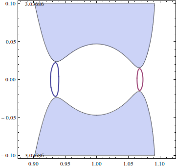
Figure 2: Projection on the plane x-y of the Lyapunov orbits related to the points $L_{1}$ and $L_{2}$, for the value $C=3.03685733643946038606918461928938$ of the Jacobi constant. The shaded area represents a region of the orbit plane which is forbidden for this value of the Jacobi constant.

The Lyapunov orbits are hyperbolic, and transverse intersections of their stable and unstable manifolds–usually called tube manifolds– produce the complicate dynamics related to the heteroclinic chaos. The numerical computation of the tube manifolds has been afforded in several papers, and has important implications also for modern space mission design (see [29], [18]).

In this Section we analyze the FLI method for the detection of the tube manifolds introduced in [24, 15] at the light of the theoretical analysis performed in Section 2, and we show that the method allows for a detection of the manifolds with a number of precision digits which increase linearly with respect to the integration time. Moreover, the modified FLI allows us to compute the manifolds with a precision limited only by the round–off of the numerical computations.

We report here three numerical experiments. In the first one we illustrate the numerical precision of the FLI method in the determination of the stable tube manifold of a Lyapunov periodic orbit around $L_{1}$; in the second one, we provide some snapshots of the stable tube manifold of the Lyapunov periodic orbit around $L_{2}$ and the unstable tube manifold of the Lyapunov periodic orbit around $L_{1}$, obtained by extending the integration time; in the third one we illustrate the numerical precision of the FLI method for the localization of a heteroclinic intersection between these two manifolds. We remark that these computations are particularly critical since the tube manifolds are located in a region of the phase space close to the singularity at $(x,y)=(1-\mu,0)$. In these circumstances, the numerical computation of both equations of motions (23) and their variational equations becomes critical, and several approaches have been introduced (see [32, 23, 3, 15]).

For the computation of the tube manifolds, we find particularly useful to define the variational equation in the space of the variables obtained by regularizing equations (23) with respect to the secondary mass, as in [3, 15]. Precisely, we consider the Levi–Civita regularization defined by the space transformation

$$\left\{\begin{array}[]{lll}x-(1-\mu)&=&u_{1}^{2}-u_{2}^{2}\\ y&=&2u_{1}u_{2}\\ \end{array}\right.$$ (25)

and by the fictitious time $s$ related to $t$ by $dt=r_{2}ds$. The equations of motion in the variables $u_{1},u_{2}$, and fictitious time $s$ are (see for example [30]):

$$\left\{\begin{array}[]{lll}u_{1}^{\prime\prime}&=&{1\over 4}[(a+b)u_{1}+cu_{2}]\\ u_{2}^{\prime\prime}&=&{1\over 4}[(a-b)u_{2}+cu_{1}]\\ \end{array}\right.$$ (26)

with:

$$\left\{\begin{array}[]{lll}a&=&{\frac{2(1-\mu)}{r_{1}}}-C+x^{2}+y^{2}\\ b&=&4y^{\prime}+2r_{2}x-{\frac{2(1-\mu)r_{2}(x-1+\mu)}{r_{1}^{3}}}\\ c&=&2r_{2}y-4x^{\prime}-{\frac{2(1-\mu)r_{2}y}{r_{1}^{3}}}\end{array}\right.$$ (27)

where $C$ denotes the value of the Jacobi constant, and the primed derivatives denote derivatives with respect the fictitious time $s$. To define the FLI, we first write (26) as a system of first order differential equations:

$$\left\{\begin{array}[]{lll}u^{\prime}_{1}&=&v_{1}\\ u^{\prime}_{2}&=&v_{2}\\ v_{1}^{\prime}&=&{1\over 4}[(a+b)u_{1}+cu_{2}]\\ v_{2}^{\prime}&=&{1\over 4}[(a-b)u_{2}+cu_{1}]\\ \end{array}\right.$$ (28)

and we introduce its compact form:

$$\xi^{\prime}=F(\xi)\\$$ (29)

with $\xi=(u_{1},u_{2},v_{1},v_{2})$. The variational equations of (29) are therefore:

$$\left\{\begin{array}[]{lcr}&\xi^{\prime}=F(\xi)&\cr&w^{\prime}={\partial F\over\partial\xi}(\xi)w&,\end{array}\right.$$ (30)

where $w\in\mathbb{R}^{4}$ represents a tangent vector. Following [15], we here consider the regularized FLI indicator defined by

$$FLI(\xi(0),w(0),T)=\log\left\|w({s(T)})\right\|$$ (31)

where $\xi(s),w(s)$ denotes the solution of the variational equations (30) with initial condition $\xi(0),w(0)$ and $s(T)$ is the fictitious time which corresponds to the physical time $T$ for that orbit. The indicator (31) will be computed also for negative times $T<0$.

FLI detection of the tube manifolds. In order to test the precision of the FLI method in the localization of the tube manifolds, we consider a point $z_{s}=(x_{s},y_{s},\dot{x}_{s},\dot{y}_{s})\in W^{s}_{L_{1}}$ in the stable tube manifold of the Lyapunov orbit around $L_{1}$ (see Figure 3), and we compute the traditional and modified FLIs for a set of many initial conditions. with $(x(0),y(0))=(x_{s},\dot{x}_{s})$ (see Fig.3), $\log\left|y(0)-y_{s}\right|$ in the interval $[-25,-1]$ and $y(0)$ obtained from the value of the Jacobi constant $C=3.03685733643946038606918461928938$. The integration times are respectively $T=15$ and $T=25$. We appreciate a localization of the manifold determined by a linear decrement of the FLI with respect to $\log\left|y(0)-y_{s}\right|$. The time $T=15$ allows us to localize the manifold with a precision of order $10^{-15}$, which is greatly improved by using $T=25$. We obtain a good localization of the manifold already with the traditional FLI, see Figure 4, although the irregularities in the FLI curve limit the precision of the localization to $10^{-22}$, higher than the numerical round–off precision.

Then, we considered a modified FLI defined by equations (8) with function $u(z)$ which is a test function of a neighbourhood of the Lyapunov orbit $\gamma_{1}$ around $L_{1}$. Precisely, we use a test function defined by:

$$u(z)=\left\{\begin{array}[]{lcr}&1&\ {\rm if}\ \ \left|z-\gamma_{1}\right|\leq{r_{1}\over 2}\\ &{1\over 2}[{\cos(({\left|z-\gamma_{1}\right|\over r_{1}}-{1\over 2})\pi)+1}]&{\rm if}\ \ {r_{1}\over 2}<\left|z-\gamma_{1}\right|\leq{3r_{1}\over 2}\\ &0&\ {\rm if}\ \ \left|z-\gamma_{1}\right|>{3r_{1}\over 2}\end{array}\right.$$ (32)

where $\left|z-\gamma_{1}\right|$ denotes the distance between $z$ and the Lyapunov orbit $\gamma_{1}$ (we set $r_{1}=10^{-3}$ in the following computations). Also in this case the time $T=15$ allows us to localize the manifold with a precision of order $10^{-15}$, while the time $T=25$ allows us to localize the manifold more precisely than $10^{-25}$. The use of the modified FLI has eliminated the irregularities in the curves of Figure 4, and improved the precision of the localization. As a matter of fact, the precision of the localization is reduced to the round–off used for the numerical computation.

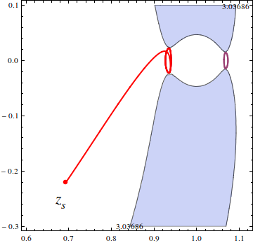
Figure 3: Projection on the plane $(x,y)$ of an orbit with initial condition $z_{s}=(x_{s},y_{s},\dot{x}_{s},\dot{y}_{s})\in W^{s}_{L_{1}}$, with $x^{s}=0.687020836763335598413507147121355$, $y^{s}=-0.227669455733293321520979535995733$, $\dot{x}^{s}=0.331597964276881596512604348842892$, and $\dot{y}^{s}$ obtained from the Jacobi constant $C=3.03685733643946038606918461928938$. The shaded area represents a region of the orbit plane which is forbidden for the value $C$ of the Jacobi constant.

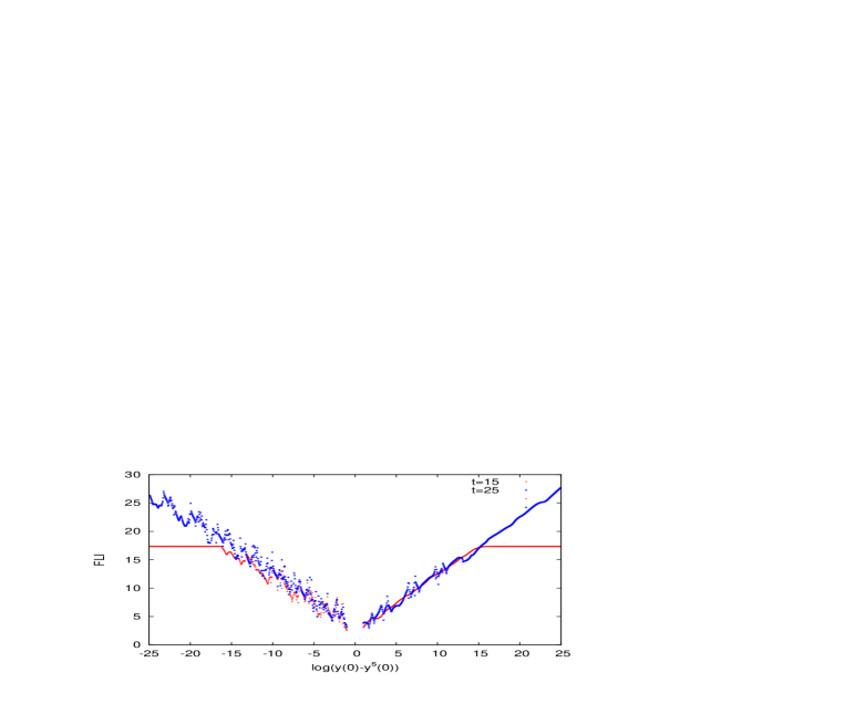
Figure 4: Values of the traditional FLI computed on a set of 960 initial conditions with $(x(0),y(0))=(x_{s},\dot{x}_{s})$ (see Fig.3), $\log\left|y(0)-y_{s}\right|$ in the interval $[-25,-1]$ and $\dot{y}(0)$ obtained from the Jacobi constant $C=3.03685733643946038606918461928938$. The integration times are respectively $T=15$ and $T=25$, (the negative values correspond to initial conditions with $y(0)<y^{s}$). We appreciate a localization of the manifold determined by a linear decrement of the FLI with respect to $\log\left|y(0)-y_{s}\right|$. The time $T=15$ allows us to localize the manifold with a precision of order $10^{-15}$, while the time $T=25$ allows us to localize the manifold more precisely than $10^{-22}$.

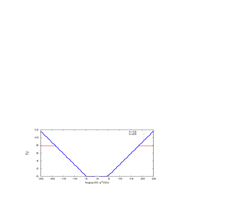
Figure 5: Values of the modified FLI defined by equations (8) with function $u(z)$ which is a test function of a neighbourhood of the Lyapunov orbit around $L_{1}$. The initial conditions are the same 960 initial conditions considered in Figure 4, that is $(x(0),y(0))=(x_{s},\dot{x}_{s})$ (see Fig.3), $\log\left|y(0)-y_{s}\right|$ in the interval $[-25,-1]$ and $y(0)$ obtained from the Jacobi constant $C=3.03685733643946038606918461928938$. The integration times are respectively $T=15$ and $T=25$, (the negative values correspond to initial conditions with $y(0)<y_{s}$). We appreciate a localization of the manifold determined by a linear decrement of the FLI with respect to $\log\left|y(0)-y_{s}\right|$. The time $T=15$ allows us to localize the manifold with a precision of order $10^{-15}$, while the time $T=25$ allows us to localize the manifold more precisely than $10^{-25}$. The use of the modified FLI has eliminated the irregularities in the curves of Figure 4, and improved he precision of the localization. As a matter of fact, the precision of the localization is reduced to the round–off used for the numerical computation.

Snapshots of tube manifolds of $W^{u}_{L_{1}}$ and $W^{s}_{L_{2}}$. Motivated by these results, we obtained sharp representations of the intersections

$$W^{s}_{L_{2}}\cap\Sigma\ \ ,\ \ W^{u}_{L_{1}}\cap\Sigma$$

of the stable tube manifold $W^{s}_{L_{2}}$ of the Lyapunov orbit $\gamma_{2}$ around $L_{2}$ and of the unstable tube manifold $W^{u}_{L_{1}}$ of the Lyapunov orbit $\gamma_{1}$ around $L_{1}$ with the two–dimensional section of the phase–space defined by

$$\Sigma=\{(x,y,\dot{x},\dot{y}):\ \ y=0\ \ ,\ \ \dot{y}\geq 0:\ \ {\cal C}(x,0,\dot{x},\dot{y})=C\}.$$ (33)

Any point $z\in\Sigma$ is parameterized and identified by its two components $(x,\dot{x})$. The representation of the manifolds are obtained by computing the modified FLIs on refined grids of initial conditions $(x,\dot{x})$ on $\Sigma$ for different integration times $T$. The stable manifold $W^{s}_{L_{2}}$ is obtained by computing the modified FLI on a time $T_{2}$, using a test function defined by

$$u(z)=\left\{\begin{array}[]{lcr}&1&\ {\rm if}\ \ \left|z-\gamma_{2}\right|\leq{r_{2}\over 2}\\ &{1\over 2}[{\cos(({\left|z-\gamma_{2}\right|\over r_{2}}-{1\over 2})\pi)+1}]&{\rm if}\ \ {r_{2}\over 2}<\left|z-\gamma_{2}\right|\leq{3r_{2}\over 2}\\ &0&\ {\rm if}\ \ \left|z-\gamma_{2}\right|>{3r_{2}\over 2}\end{array}\right.$$ (34)

where $\left|z-\gamma_{2}\right|$ denotes the distance between $z$ and the Lyapunov orbit $\gamma_{2}$ and $r_{2}=5\,10^{-4}$. The unstable manifold $W^{u}_{L_{1}}$ is obtained by computing the modified FLI on a negative time $-T_{1}$, using a test function defined by

$$u(z)=\left\{\begin{array}[]{lcr}&1&\ {\rm if}\ \ \left|z-\gamma_{1}\right|\leq{r_{1}\over 2}\\ &{1\over 2}[{\cos(({\left|z-\gamma_{1}\right|\over r_{1}}-{1\over 2})\pi)+1}]&{\rm if}\ \ {r_{1}\over 2}<\left|z-\gamma_{1}\right|\leq{3r_{1}\over 2}\\ &0&\ {\rm if}\ \ \left|z-\gamma_{1}\right|>{3r_{1}\over 2}\end{array}\right.$$ (35)

where $\left|z-\gamma_{1}\right|$ denotes the distance between $z$ and the Lyapunov orbit $\gamma_{1}$ and $r_{1}=10^{-3}$. In such a way, for any $x,\dot{x}$ we compute the modified FLIs: FLI₁, FLI₂. The representation of both manifolds on the same picture is obtained by representing with a color scale a weighted average of the two indicators:

$${w{\rm FLI}_{1}+{\rm FLI}_{2}\over(w+1)}.$$ (36)

The results are represented in Figures 6 and 7 for $T=5$ and $T=100$ respectively. We clearly appreciate different lobes of both manifolds already for the shorter integration time $T=5$. The longer time $T=100$ allows us to appreciate additional lobes, which contain initial condition approaching the manifolds only after several revolution periods of Jupiter.

Figure 6: Representation of the modified FLIs computed on a grid of $4000\times 4000$ initial conditions regularly spaced on $(x,\dot{x})$ (the axes on the picture–the other initial conditions are $y=0$ and $\dot{y}$ is computed from the Jacobi constant $C=3.0368573364394607$), computed with integration time $T=5$. In order to represent both manifolds on the same picture, we represent with a color scale the weighted average (36) of the two indicators ${\rm FLI}_{1}$, ${\rm FLI}_{2}$ with weight $w=100$. The yellow curves on the picture correspond to different lobes of the manifolds.

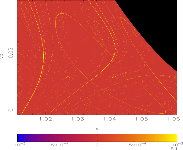
Figure 7: Representation of the modified FLIs computed on a grid of $4000\times 4000$ initial conditions regularly spaced on $(x,\dot{x})$ (the axes on the picture–the other initial conditions are $y=0$ and $\dot{y}$ is computed from the Jacobi constant $C=3.0368573364394607$), computed with an integration time $T=100$. In order to represent both manifolds on the same picture, we represent with a color scale the weighted average (36) of the two indicators ${\rm FLI}_{1}$, ${\rm FLI}_{2}$ with weight $w=500$. The yellow curves on the picture correspond to different lobes of the manifolds. Due to the integration time which is much longer than the time used in Figure 6, many additional lobes of the tube manifolds of both $\gamma_{1}$ and $\gamma_{2}$ appear on this figure. Their corresponding initial conditions approach the manifolds only after several revolution periods of Jupiter.

Localization of heteroclinic intersections. The detection of both manifolds $W^{u}_{L_{1}}$ and $W^{s}_{L_{2}}$ on the same picture (see Figure 6 and Figure 7) allows us to obtain a precise localization of the heteroclinic intersections points, which we denote by $z_{he}$. Precisely, the intersection between the two yellow curves in the box of Fig.6 corresponds to an intersection point $z_{he}$. Of course, accordingly to the resolution of the computation, at first we are only able to determine a point $z_{he,1}$ in the box which is close $z_{he}$. To improve the localization of $z_{he}$ we compute again the modified FLIs on a refined grid of points in the box of Fig.6, and we obtain a new point $z_{he,2}$ (the point with the maximum value of the averaged FLI (36)) closer to the intersection point. The procedure is iterated by computing again the FLIs on zoomed out grids of initial conditions centered on $z_{he,j}$ with $j=2,...15$, with increasing integration times to increase the number of precision digits in the localization of the heteroclinic point.

In Fig.8 we plot the FLI values computed on a grid of $500\times 500$ initial conditions centered on the point $z_{he,15}$, using the integration time $T=18$. The maximum value of the FLI in this picture provides a new refined initial condition that we used to compute the heteroclinic orbit shown in Fig.9. The convergence of the forward (backward) integration towards the Lyapunov orbit related to $L_{2}$ ($L_{1}$) clearly shows the validity of the method for the precise localization of heteroclinic orbits.

Figure 8: Computation of the averaged FLI (36) on a grid of $500\times 500$ initial conditions centered on the point $z_{he,15}$ of coordinates: $x_{he,15}=1.041239777351473900$, $y_{he,15}=0$, $\dot{x}_{he,15}=0.0460865533656582000$. The velocity $\dot{y}_{he,15}$ is obtained from the Jacobi constant $C=3.0368573364394607$. The integration time is $T=18$. The values of the FLI are provided as the average between FLI₁ and FLI₂. A sharp detection of both manifolds appears thanks to the differentiation of the FLI values on this refined grid. The maximum value of the FLI in this picture provides a new refined initial condition for the orbit plotted in Fig.9.

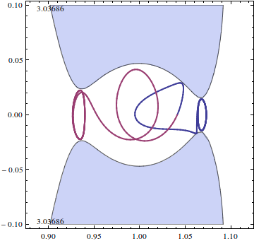
Figure 9: Projection on the plane $(x,y)$ of the heteroclinic orbit found through the maximum of the FLI (see text). The conditions are : $x_{he}(0)=1.041239777351473912$, $y_{he}(0)=0$, $\dot{x}_{he}(0)=0.046086553365658360$ and $\dot{y}_{he}(0)$ obtained from the Jacobi constant $C=3.0368573364394607$. Blue points: forward integration, the orbit converges to the Lyapunov orbit related to $L_{2}$. Red points: backward integration, the orbit converges to the Lyapunov orbit related to $L_{1}$.

4 Proofs

Proof of Proposition 1. We first remark that (15) implies $\varepsilon_{0}\leq\varepsilon_{1}$, and condition (16) implies

$$\varepsilon_{0}\leq{\delta_{0}^{2}\over\max(1,\eta)(1+\lambda_{w})\lambda^{T_{s}}T^{2}}.$$

The proof of Proposition 1 is a consequence of the following:

Lemma 4.1

For any $\varepsilon,\delta$ satisfying

$$\max(1,\eta)(1+\lambda_{w})\lambda^{T_{s}}\varepsilon\leq\delta^{2}$$ (37)

$$\delta\leq\min\left({1\over 2}\ ,\ {r_{*}\over 2}\ ,\ {1\over\eta}\ ,\ {1\over 4e^{2}\lambda_{u}\eta}\Big{(}1-{1\over\lambda_{u}}\Big{)}\ ,\ {1\over 2e^{3}\lambda_{u}^{2}\eta}{1\over T_{\varepsilon}}\right)$$ (38)

we have:

$$\delta-\eta\Delta_{\varepsilon}\leq\left|\Phi^{T_{s}+T_{\varepsilon}}_{1}(z_{\varepsilon})\right|\leq e^{2}\lambda_{u}\delta+\eta\Delta_{\varepsilon}$$ (39)

$$\left|\Phi^{T_{s}+T_{\varepsilon}}_{2}(z_{\varepsilon})\right|\leq e^{2}\lambda_{u}\delta+2\eta\Delta_{\varepsilon}$$ (40)

$$\left|\Phi^{T_{s}+T_{\varepsilon}}_{2}(z_{\varepsilon})-(\zeta_{\varepsilon})_{2}\right|\leq{1\over\lambda_{u}^{T_{\varepsilon}}}4e^{3}\lambda_{u}\delta$$ , (41)

and the tangent vector $D\Phi^{T_{s}+T_{\varepsilon}}_{z_{\varepsilon}}v$ satisfies

$$\left\|D\Phi^{T_{s}+T_{\varepsilon}}_{z_{\varepsilon}}v-A^{T_{\varepsilon}}(w_{u}+w_{s})\right\|\leq\lambda_{u}^{T_{\varepsilon}}\delta\left(\eta\max(e,\eta){4e^{2}\lambda_{u}^{2}\over\lambda_{u}-1}+1\right)\left\|w_{u}\right\|.$$ (42)

First, as we anticipated in Section 2, the time $T_{\varepsilon}$ can be identified as the time required by the orbit with initial condition $\Phi^{T_{s}}(z_{\varepsilon})$ to exit from $B(\delta)$ and to arrive at the small distance $(4e^{3}\lambda_{u}\delta)/\lambda_{u}^{T_{\varepsilon}}$ from the local unstable manifold. If $T_{\varepsilon}\geq T-T_{s}$, we can repeat the proof of Lemma 4.1 by limiting all the estimates to the time interval $[0,T]$, and obtaining

$$\left\|D\Phi^{T}_{z_{\varepsilon}}v-A^{T-T_{s}}w\right\|\leq\lambda_{u}^{T-T_{s}}\delta\left(\eta\max(e,\eta){4e^{2}\lambda_{u}^{2}\over\lambda_{u}-1}+1\right)\left\|w_{u}\right\|,$$ (43)

so that (19) is proved. If $T_{\varepsilon}<T-T_{s}$, we need an estimate of the growth of the tangent vectors in the remaining time interval $[T_{s}+T_{\varepsilon},T]$, and we obtain it by comparison with the growth of the tangent vectors of the orbits with initial condition in the point $\zeta_{\varepsilon}$ on the unstable manifold. We will provide estimates of the FLI for $T_{\varepsilon}$ in the interval:

$$(T-T_{s}(\delta)){\ln\lambda\over\ln\lambda+\ln\lambda_{u}}\leq T_{\varepsilon}<T-T_{s}(\delta).$$ (44)

Let us consider $j=T-T_{s}-T_{\varepsilon}\in\{1,(T-T_{s}(\delta)){\ln\lambda_{u}\over\ln\lambda+\ln\lambda_{u}}\}$. First, we have

$$\left\|D\Phi^{T}_{z_{\varepsilon}}v-D\Phi^{j}_{\zeta_{\varepsilon}}D\Phi^{T_{s}+T_{\varepsilon}}_{z_{\varepsilon}}v\right\|\leq 4e^{3}\lambda_{u}{\lambda^{j}\over\lambda_{u}^{T_{\varepsilon}}}\delta\left\|D\Phi^{j}_{\zeta_{\varepsilon}}D\Phi^{T_{s}+T_{\varepsilon}}_{z_{\varepsilon}}v\right\|,$$ (45)

In fact, since

$$D\Phi^{T}_{z_{\varepsilon}}v=D\Phi^{j}_{\Phi^{T_{s}+T_{\varepsilon}}(z_{\varepsilon})}D\Phi^{T_{s}+T_{\varepsilon}}_{z_{\varepsilon}}v=D\Phi^{j}_{\zeta_{\varepsilon}}D\Phi^{T_{s}+T_{\varepsilon}}_{z_{\varepsilon}}v+\Big{(}D\Phi^{j}_{\Phi^{T_{s}+T_{\varepsilon}}(z_{\varepsilon})}-D\Phi^{j}_{\zeta_{\varepsilon}}\Big{)}D\Phi^{T_{s}+T_{\varepsilon}}_{z_{\varepsilon}}v,$$

using Lemmas 4.1 and 5.2 we obtain

$$\left\|D\Phi^{T}_{z_{\varepsilon}}v-D\Phi^{j}_{\zeta_{\varepsilon}}D\Phi^{T_{s}+T_{\varepsilon}}_{z_{\varepsilon}}v\right\|\leq\lambda^{j}\left\|\Phi^{T_{s}+T_{\varepsilon}}_{z_{\varepsilon}}-\zeta_{\varepsilon}\right\|\left\|D\Phi^{j}_{\zeta_{\varepsilon}}D\Phi^{T_{s}+T_{\varepsilon}}_{z_{\varepsilon}}v\right\|\leq 4e^{3}\lambda_{u}{\lambda^{j}\over\lambda_{u}^{T_{\varepsilon}}}\delta\left\|D\Phi^{j}_{\zeta_{\varepsilon}}D\Phi^{T_{s}+T_{\varepsilon}}_{z_{\varepsilon}}v\right\|.$$

Therefore, we have

$$\left\|D\Phi^{T}_{z_{\varepsilon}}v\right\|\leq\left\|D\Phi^{j}_{\zeta_{\varepsilon}}D\Phi^{T_{s}+T_{\varepsilon}}_{z_{\varepsilon}}v\right\|\left(1+4e^{3}\lambda_{u}{\lambda^{j}\over\lambda_{u}^{T_{\varepsilon}}}\delta\right).$$

We now analyze and compare the FLI for initial conditions at different distances from the stable manifold. We have

$${\left\|D\Phi^{T}_{z_{\varepsilon}}v\right\|\over\left\|D\Phi^{T}_{z_{s}}v\right\|}\leq{\left\|D\Phi^{j}_{\zeta_{\varepsilon}}D\Phi^{T_{s}+T_{\varepsilon}}_{z_{\varepsilon}}v\right\|\over\left\|D\Phi^{T}_{z_{s}}v\right\|}\left(1+4e^{3}\lambda_{u}{\lambda^{j}\over\lambda_{u}^{T_{\varepsilon}}}\delta\right).$$

Using inequalities (43) and (42), we obtain

$${\left\|D\Phi^{T}_{z_{\varepsilon}}v\right\|\over\left\|D\Phi^{T}_{z_{s}}v\right\|}\leq{\left\|D\Phi^{j}_{\zeta_{\varepsilon}}\right\|\over\lambda_{u}^{j}}\ {1+\delta\left(\eta\max(e,\eta){4e^{2}\lambda_{u}^{2}\over\lambda_{u}-1}+1\right)\over 1-\delta\left(\eta\max(e,\eta){4e^{2}\lambda_{u}^{2}\over\lambda_{u}-1}+1\right)}\left(1+4e^{3}\lambda_{u}{\lambda^{j}\over\lambda_{u}^{T_{\varepsilon}}}\delta\right).$$ (46)

In fact, from (43) and $\left\|A^{T-T_{s}}(w_{u}+w_{s})\right\|=\lambda_{u}^{T-T_{s}}\left\|w_{u}\right\|$, we obtain that for all $\varepsilon$ with $T_{\varepsilon}\geq T-T_{s}$, including $z_{0}=z_{s}$, we have

$$\left\|D\Phi^{T}_{z_{\varepsilon}}v\right\|\geq\lambda_{u}^{T-T_{s}}\left(1-\delta\left(\eta\max(e,\eta){4e^{2}\lambda_{u}^{2}\over\lambda_{u}-1}+1\right)\right)\left\|w_{u}\right\|.$$ (47)

From (42), for all $\varepsilon$ with $T_{\varepsilon}\leq T-T_{s}$, we have:

$$\left\|D\Phi^{j}_{\zeta_{\varepsilon}}D\Phi^{T_{s}+T_{\varepsilon}}_{z_{\varepsilon}}v\right\|\leq\left\|D\Phi^{j}_{\zeta_{\varepsilon}}\right\|\left\|D\Phi^{T_{s}+T_{\varepsilon}}_{z_{\varepsilon}}v\right\|$$

$$\leq\left\|D\Phi^{j}_{\zeta_{\varepsilon}}\right\|\left(\left\|A^{T_{\varepsilon}}w\right\|+\lambda_{u}^{T_{\varepsilon}}\delta\left(\eta\max(e,\eta){4e^{2}\lambda_{u}^{2}\over\lambda_{u}-1}+1\right)\left\|w\right\|\right)$$

$$\leq\left\|D\Phi^{j}_{\zeta_{\varepsilon}}\right\|\lambda_{u}^{T_{\varepsilon}}\left\|w_{u}\right\|\left(1+\delta\left(\eta\max(e,\eta){4e^{2}\lambda_{u}^{2}\over\lambda_{u}-1}+1\right)\right).$$ (48)

Since for all $\varepsilon$ with

$$T_{\varepsilon}\geq(T-T_{s}){\ln\lambda\over\ln\lambda+\ln\lambda_{u}},$$

we have

$${\lambda^{j}\over\lambda_{u}^{T_{\varepsilon}}}={\lambda^{T-T_{s}-T_{\varepsilon}}\over\lambda_{u}^{T_{\varepsilon}}}\leq 1,$$

using also

$$\delta\left(\eta\max(e,\eta){4e^{2}\lambda_{u}^{2}\over\lambda_{u}-1}+1\right)\leq{1\over 2eT}\ ,\ 4e^{3}\lambda_{u}\delta<{1\over 4T}$$

we have

$${1+\delta\left(\eta\max(e,\eta){4e^{2}\lambda_{u}^{2}\over\lambda_{u}-1}+1\right)\over 1-\delta\left(\eta\max(e,\eta){4e^{2}\lambda_{u}^{2}\over\lambda_{u}-1}+1\right)}\left(1+4e^{3}\lambda_{u}{\lambda^{j}\over\lambda_{u}^{T_{\varepsilon}}}\delta\right)\leq\left(1+{1\over T}\right),$$

so that, from (46), we immediately obtain (20).

Proof of (13). We have:

$$\Delta_{\varepsilon}=\left|\Phi^{T_{s}}_{1}(z_{\varepsilon})-w_{s}(\Phi^{T_{s}}_{2}(z_{\varepsilon}))\right|\leq\left|\Phi^{T_{s}}_{1}(z_{\varepsilon})-\Phi^{T_{s}}_{1}(z_{s})\right|+\left|w_{s}(\Phi^{T_{s}}_{2}(z_{s}))-w_{s}(\Phi^{T_{s}}_{2}(z_{\varepsilon}))\right|$$

$$\leq\lambda_{\Phi}^{T_{s}}\varepsilon+\lambda_{w}\lambda_{\Phi}^{T_{s}}\varepsilon\leq(1+\lambda_{w})\lambda_{\Phi}^{T_{s}}\varepsilon.$$

Proof of Lemma 4.1. We consider the segments which join $\Phi^{k}(\pi_{\varepsilon})$ and $\Phi^{k}(\Phi^{T_{s}}(z_{\varepsilon}))$, and define

$$\Delta^{k}_{1}=\left|\Phi^{k}_{1}(\Phi^{T_{s}}(z_{\varepsilon}))-\Phi^{k}_{1}(\pi_{\varepsilon})\right|$$

$$\Delta^{k}_{2}=\left|\Phi^{k}_{2}(\Phi^{T_{s}}(z_{\varepsilon}))-\Phi^{k}_{2}(\pi_{\varepsilon})\right|.$$

We prove that, for all the $k$ such that $\Phi^{k}(\pi_{\varepsilon}),\Phi^{k}(\Phi^{T_{s}}(z_{\varepsilon}))\leq B(A\delta)$, for $A>1$, we have

$$\Delta^{k}_{2}<\Delta^{k}_{1}.$$

In fact, we have $\Delta^{0}_{1}=\Delta_{\varepsilon}$, $\Delta^{0}_{2}=0$; then, if $\Delta^{k-1}_{2}<\Delta^{k-1}_{1}$, we have

$$\Delta^{k}_{2}=\left|\Phi^{k}_{2}(\Phi^{T_{s}}(z_{\varepsilon}))-\Phi^{k}_{2}(\pi_{\varepsilon})\right|=\left|\Phi_{2}(\Phi^{k-1}(\Phi^{T_{s}}(z_{\varepsilon})))-\Phi_{2}(\Phi^{k-1}(\pi_{\varepsilon}))\right|$$

$$\leq{1\over\lambda_{u}}\Delta^{k-1}_{2}+\left|f_{2}(\Phi^{k-1}(\Phi^{T_{s}}(z_{\varepsilon})))-f_{2}(\Phi^{k-1}(\pi_{\varepsilon}))\right|$$

$$\leq{1\over\lambda_{u}}\Delta^{k-1}_{2}+A\eta\delta(\Delta^{k-1}_{1}+\Delta^{k-1}_{2})\leq\Big{(}{1\over\lambda_{u}}+2A\eta\delta\Big{)}\Delta^{k-1}_{1}<\Delta^{k-1}_{1}$$

as soon as

$${1\over\lambda_{u}}+2A\eta\delta<1.$$

Therefore, we have

$$\Delta^{k}_{1}=\left|\Phi^{k}_{1}(\Phi^{T_{s}}(z_{\varepsilon}))-\Phi^{k}_{1}(\pi_{\varepsilon})\right|\leq\lambda_{u}\Delta^{k-1}_{1}+A\eta\delta(\Delta^{k-1}_{1}+\Delta^{k-1}_{2})$$

$$\leq(\lambda_{u}+2\eta A\delta)\Delta^{k-1}_{1}\leq(\lambda_{u}+2\eta A\delta)^{k}\Delta^{0}_{1}=\lambda_{u}^{k}\Big{(}1+{2\eta A\delta\over\lambda_{u}}\Big{)}^{k}\Delta_{\varepsilon}\leq e\lambda_{u}^{k}\Delta_{\varepsilon}$$

and

$$\Delta^{k}_{1}\geq\lambda_{u}\Delta^{k-1}_{1}-A\eta(\Delta^{k-1}_{1}+\Delta^{k-1}_{2})\geq(\lambda_{u}-2A\eta\delta)\Delta^{k-1}_{1}$$

$$\geq\lambda_{u}^{k}\Big{(}1-{2\eta A\delta\over\lambda_{u}}\Big{)}^{k}\Delta_{\varepsilon}\geq{1\over e}\lambda_{u}^{k}\Delta_{\varepsilon}$$

as soon as $k\leq T$ and

$${2\eta A\delta\over\lambda_{u}}\leq{1\over 2k}.$$

We obtained

$${1\over e}\lambda_{u}^{k}\Delta_{\varepsilon}\leq\Delta^{k}_{1}\leq e\lambda_{u}^{k}\Delta_{\varepsilon}.$$

We now provide an estimate of $\Phi^{k}_{1}(\pi_{\varepsilon})$ and $\Phi^{k}_{2}(\pi_{\varepsilon})$. We consider the segment which joins the origin $(0,0)$ and $\Phi^{k}(\pi_{\varepsilon})$ and define

$$\delta_{1}^{k}=\left|\Phi^{k}_{1}(\pi_{\varepsilon})\right|\ \ ,\ \ \delta_{2}^{k}=\left|\Phi^{k}_{2}(\pi_{\varepsilon})\right|.$$

We have $\delta_{1}^{k}<\delta_{2}^{k}$ for any $k$. In fact, since $\pi_{\varepsilon}\in B(\delta)$ and $\pi_{\varepsilon}\in W^{l}_{s}$, then $\Phi^{k}(\pi_{\varepsilon})\in B(\delta)$ for any $k$ and we have

$$\delta_{1}^{k}=\left|\Phi^{k}_{1}(\pi_{\varepsilon})\right|=\left|w_{s}(\Phi^{k}_{2}(\pi_{\varepsilon}))\right|\leq\eta\left|\Phi^{k}_{2}(\pi_{\varepsilon})\right|^{2}\leq\eta\delta\delta^{k}_{2}<\delta^{k}_{2}$$

as soon as

$$\eta\delta<1.$$

For $k=0$ we have

$$\delta_{1}^{0}=\left|(\pi_{\varepsilon})_{1}\right|=\left|w_{s}((\pi_{\varepsilon})_{2})\right|\leq\eta\left|\Phi^{T_{s}}_{2}(z_{s})\right|^{2}\leq\eta\delta\left|\Phi^{T_{s}}_{2}(z_{s})\right|\leq\eta\delta^{2}\ \ ,\ \ \delta_{2}^{0}=\left|\Phi^{T_{s}}_{2}(z_{s})\right|\leq\delta$$

Then, we have

$$\delta_{2}^{k}=\left|\Phi^{k}_{2}(\pi_{\varepsilon})\right|=\left|\Phi_{2}(\Phi^{k-1}(\pi_{\varepsilon}))\right|\leq{1\over\lambda_{u}}\left|\Phi^{k-1}_{2}(\pi_{\varepsilon})\right|+\eta\left\|\Phi^{k-1}(\pi_{\varepsilon})\right\|^{2}\leq{1\over\lambda_{u}}\delta_{2}^{k-1}+\eta(\delta_{2}^{k-1})^{2}$$

$$\leq\Big{(}{1\over\lambda_{u}}+\eta\delta\Big{)}\delta_{2}^{k-1}\leq\Big{(}{1\over\lambda_{u}}+\eta\delta\Big{)}^{k}\delta_{2}^{0}\leq{1\over\lambda_{u}^{k}}\Big{(}1+\eta\lambda_{u}\delta\Big{)}^{k}\delta\leq{1\over\lambda_{u}^{k}}e\delta$$

as soon as

$$\eta\lambda_{u}\delta\leq{1\over ek},$$

and

$$\delta_{1}^{k}=\left|w_{s}(\Phi^{k}_{2}(\pi_{\varepsilon})\right|\leq\eta\left|\Phi^{k}_{2}(\pi_{\varepsilon})\right|^{2}=\eta(\delta_{2}^{k})^{2}\leq\eta e{1\over\lambda_{u}^{k}}\delta.$$

Therefore, from

$${1\over e}\lambda_{u}^{k}\Delta_{\varepsilon}\leq\left|\Phi^{k}_{1}(\Phi^{T_{s}}(z_{\varepsilon}))-\Phi^{k}_{1}(\pi_{\varepsilon})\right|\leq e\lambda_{u}^{k}\Delta_{\varepsilon}$$

we have

$${1\over e}\lambda_{u}^{k}\Delta_{\varepsilon}-\eta e{1\over\lambda_{u}^{k}}\delta\leq\left|\Phi^{k}_{1}(\Phi^{T_{s}}(z_{\varepsilon}))\right|\leq e\lambda_{u}^{k}\Delta_{\varepsilon}+\eta e{1\over\lambda_{u}^{k}}\delta.$$

Finally, from $\Delta^{k}_{2}<\Delta^{k}_{1}$ we have

$$\left|\Phi^{k}_{2}(\Phi^{T_{s}}(z_{\varepsilon}))\right|\leq\Delta^{k}_{1}+\left|\Phi^{k}_{2}(\pi_{\varepsilon})\right|\leq e\lambda_{u}^{k}\Delta_{\varepsilon}+{1\over\lambda_{u}^{k}}e\delta.$$

From the definition of $T_{\varepsilon}$, we have

$${e\delta\over\Delta_{\varepsilon}}\leq\lambda_{u}^{T_{\varepsilon}}<{\lambda_{u}e\delta\over\Delta_{\varepsilon}},$$

and therefore we have

$$\delta-\eta\Delta_{\varepsilon}\leq\delta-\eta e{\delta\over\lambda_{u}^{T_{\varepsilon}}}\leq\left|\Phi^{k}_{1}(\Phi^{T_{s}}(z_{\varepsilon}))\right|\leq e^{2}\lambda_{u}\delta+\eta\Delta_{\varepsilon}$$

$$\left|\Phi^{k}_{2}(\Phi^{T_{s}}(z_{\varepsilon}))\right|\leq e^{2}\lambda_{u}\delta+2\eta\Delta_{\varepsilon}.$$

Therefore, since $\Delta_{\varepsilon}\leq(1+\lambda_{w})\lambda_{\Phi}^{T_{s}}\varepsilon$, as soon as

$$\max(1,\eta)(1+\lambda_{w})\lambda^{T_{s}}\varepsilon<\delta^{2}$$

we have

$$\left\|\Phi^{k}(\Phi^{T_{s}}(z_{\varepsilon}))\right\|\leq e^{2}\lambda_{u}\delta+2\eta\Delta_{\varepsilon}\leq e^{2}\lambda_{u}\delta+2\eta(1+\lambda_{w})\lambda_{\Phi}^{T_{s}}\varepsilon<e^{2}\lambda_{u}\delta+\delta^{2}<2e^{2}\lambda_{u}\delta=A\delta$$

for $A=2e^{2}\lambda_{u}$. The thresholds conditions on $\delta$ become

$$\delta\leq{1\over 4e^{2}\lambda_{u}\eta}\Big{(}1-{1\over\lambda_{u}}\Big{)}\ \ ,\ \ \delta\leq{1\over 8e^{2}\eta}{1\over T_{\varepsilon}}\ \ ,\ \ \delta\leq{1\over 2e^{3}\lambda_{u}^{2}\eta}{1\over T_{\varepsilon}}.$$

We now consider the point

$$\zeta_{\varepsilon}=\Big{(}\Phi^{T_{s}+T_{\varepsilon}}_{1}(z_{\varepsilon}),w_{u}(\Phi^{T_{s}+T_{\varepsilon}}_{1}(z_{\varepsilon}))\Big{)}$$

and the segments which join $\Phi^{-k}(\zeta_{\varepsilon})$ and $\Phi^{-k}(\Phi^{T_{s}+T_{\varepsilon}}(z_{\varepsilon}))$, for $k\leq T_{\varepsilon}$. We already know that $\Phi^{-k}(\Phi^{T_{s}+T_{\varepsilon}}(z_{\varepsilon}))\in B(A\delta)$, and

$$\left\|\zeta_{\varepsilon}\right\|=\left\|\Big{(}\Phi^{T_{s}+T_{\varepsilon}}(z_{\varepsilon}),w_{u}(\Phi^{T_{s}+T_{\varepsilon}}(z_{\varepsilon}))\Big{)}\right\|\leq\max(A\delta,\eta A\delta^{2})\leq A\delta$$

as soon as $\eta\delta\leq 1$. By definition of local unstable manifold, we have $\Phi^{-k}(\zeta_{\varepsilon})\in B(A\delta)$. We define

$$\Delta^{-k}_{1}=\left|\Phi^{-k+T_{s}+T_{\varepsilon}}_{1}(z_{\varepsilon})-\Phi^{-k}_{1}(\zeta_{\varepsilon})\right|$$

$$\Delta^{-k}_{2}=\left|\Phi^{-k+T_{s}+T_{\varepsilon}}_{2}(z_{\varepsilon}))-\Phi^{-k}_{2}(\zeta_{\varepsilon})\right|,$$

in particular we have

$$\Delta^{0}_{1}=0\ \ ,\ \ \Delta^{0}_{2}:=\Delta^{\varepsilon}.$$

By repeating the above arguments using the inverse map $\Phi^{-1}(x)$, we have $\Delta^{-k}_{1}<\Delta^{-k}_{2}$ for any $k$ and:

$${1\over e}\lambda_{u}^{k}\Delta^{\varepsilon}\leq\Delta_{2}^{-k}\leq e\lambda_{u}^{k}\Delta^{\varepsilon}$$

$$\Delta^{\varepsilon}=\left|\Phi^{T_{s}+T_{\varepsilon}}_{2}(z_{\varepsilon})-(\zeta_{\varepsilon})_{2}\right|\leq{e\over\lambda_{u}^{T_{\varepsilon}}}\Delta_{2}^{-T_{\varepsilon}}\leq{e\over\lambda_{u}^{T_{\varepsilon}}}2A\delta.$$

It remains to prove (42). For any $k\leq T_{\varepsilon}$, we have:

$$\left\|\Phi^{k}(\Phi^{T_{s}}(z_{\varepsilon}))\right\|\leq e\lambda_{u}^{k}\Delta_{\varepsilon}+\max(1,\eta)e{1\over\lambda_{u}^{k}}\delta\leq e^{2}{\lambda_{u}\over\lambda_{u}^{T_{\varepsilon}-k}}\delta+\max(1,\eta)e{1\over\lambda_{u}^{k}}\delta$$

and

$$\sum_{k=0}^{T_{\varepsilon}-1}\left\|\Phi^{k}(\Phi^{T_{s}}(z_{\varepsilon}))\right\|\leq\sum_{k=0}^{T_{\varepsilon}-1}\left(e^{2}{\lambda_{u}\over\lambda_{u}^{T_{\varepsilon}-k}}+\max(1,\eta)e{1\over\lambda_{u}^{k}}\right)\delta$$

$$\leq 2e\lambda_{u}\max(e,\eta)\delta\sum_{k=0}^{T_{\varepsilon}}{1\over\lambda_{u}^{k}}\leq 2e\lambda_{u}\max(e,\eta){\lambda_{u}\over\lambda_{u}-1}\delta.$$

so that, by using also lemma 5.1, we have:

$$\left\|D\Phi^{T_{\varepsilon}}_{\Phi^{T_{s}}(z_{\varepsilon})}D\Phi^{T_{s}}_{z_{\varepsilon}}v-A^{T_{\varepsilon}}D\Phi^{T_{s}}_{z_{\varepsilon}}v\right\|\leq\left\|D\Phi^{T_{\varepsilon}}_{\Phi^{T_{s}}(z_{\varepsilon})}-A^{T_{\varepsilon}}\right\|\left\|D\Phi^{T_{s}}_{z_{\varepsilon}}v\right\|$$

$$\leq\eta\lambda_{u}^{T_{\varepsilon}}\left(1+2\eta e^{2}\delta\right)^{T_{\varepsilon}-1}\sum_{k=0}^{T_{\varepsilon}-1}\left\|\Phi^{k}(\Phi^{T_{s}}(z_{\varepsilon}))\right\|\left\|D\Phi^{T_{s}}_{z_{\varepsilon}}v\right\|$$

$$\leq\eta\max(e,\eta){2e^{2}\lambda_{u}^{2}\over\lambda_{u}-1}\ \lambda_{u}^{T_{\varepsilon}}\delta\left\|D\Phi^{T_{s}}_{z_{\varepsilon}}v\right\|.$$

We have

$$\left\|D\Phi^{T_{s}+T_{\varepsilon}}_{z_{\varepsilon}}v-A^{T_{\varepsilon}}w\right\|\leq\left\|D\Phi^{T_{\varepsilon}}_{\Phi^{T_{s}}(z_{\varepsilon})}D\Phi^{T_{s}}_{z_{\varepsilon}}v-A^{T_{\varepsilon}}D\Phi^{T_{s}}_{z_{\varepsilon}}v\right\|+\left\|A^{T_{\varepsilon}}(D\Phi^{T_{s}}_{z_{\varepsilon}}v-w)\right\|$$

$$\leq\eta\max(e,\eta){2e^{2}\lambda_{u}^{2}\over\lambda_{u}-1}\ \lambda_{u}^{T_{\varepsilon}}\delta\left\|D\Phi^{T_{s}}_{z_{\varepsilon}}v\right\|+\left\|A\right\|^{T_{\varepsilon}}\left\|D\Phi^{T_{s}}_{z_{\varepsilon}}v-w\right\|$$

$$\leq\eta\max(e,\eta){2e^{2}\lambda_{u}^{2}\over\lambda_{u}-1}\ \lambda_{u}^{T_{\varepsilon}}\delta\Big{(}\left\|w\right\|+\left\|D\Phi^{T_{s}}_{z_{\varepsilon}}v-w\right\|\Big{)}+{\lambda_{u}}^{T_{\varepsilon}}\left\|D\Phi^{T_{s}}_{z_{\varepsilon}}v-w\right\|$$

and using (12) and $\left\|w\right\|=\left\|w_{u}\right\|$ we obtain

$$\left\|D\Phi^{T_{s}+T_{\varepsilon}}_{z_{\varepsilon}}v-A^{T_{\varepsilon}}w\right\|\leq\lambda_{u}^{T_{\varepsilon}}\left(\eta\max(e,\eta){2e^{2}\lambda_{u}^{2}\over\lambda_{u}-1}\ \delta(1+\lambda^{T_{s}}\varepsilon)+\lambda^{T_{s}}\varepsilon\right)\left\|w_{u}\right\|$$

and, since $\lambda^{T_{s}}\varepsilon\leq\delta^{2}\leq\delta\leq 1$:

$$\left\|D\Phi^{T_{s}+T_{\varepsilon}}_{z_{\varepsilon}}v-A^{T_{\varepsilon}}(w_{u}+w_{s})\right\|\leq\lambda_{u}^{T_{\varepsilon}}\delta\left(\eta\max(e,\eta){4e^{2}\lambda_{u}^{2}\over\lambda_{u}-1}+1\right)\left\|w_{u}\right\|.$$ (49)

5 Two Technical Lemmas

In this Section we prove two technical Lemmas which we obtain by using Lipschitz inequalities for $\Phi$ and $D\Phi$.

Lemma 5.1

Let $U\subseteq{\mathbb{R}}^{n}$ be a neighbourhood of $0$, and $\Phi:U\rightarrow{\mathbb{R}}^{n}$ be a smooth map:

$$\Phi(z)=Az+f(z)$$

with $f_{i}(0,\ldots,0)=0$, ${\partial f_{i}\over\partial z_{j}}(0,\ldots,0)=0$ for any $i,j$ and, for any $z\in B(R)$, satisfying

$$\left\|f(z)\right\|\leq\eta\left\|z\right\|^{2}\ \ ,\ \ \left\|Df_{z}\right\|\leq\eta\left\|z\right\|\ \ ,\ \ \left\|D\Phi_{z}\right\|\leq l.$$

Then, for any $z,K$ such that $\Phi^{k}(z)\in B(R)$ for any $k=0,\ldots,K$, we have

$$\left\|D\Phi^{k}_{z}-A^{k}\right\|\leq\eta\sum_{j=0}^{k-1}\lambda_{u}^{j}\left\|\Phi^{j}(z)\right\|\left(\lambda_{u}+\eta\left\|\Phi^{j+1}(z)\right\|\right)\ldots\left(\lambda_{u}+\eta\left\|\Phi^{k-1}(z)\right\|\right)$$ (50)

and

$$\left\|D\Phi^{k}_{z}-A^{k}\right\|\leq\eta\Big{(}\lambda_{u}+\eta\max_{j\leq k-1}\left\|\Phi^{j}(z)\right\|\Big{)}^{k-1}\sum_{j=0}^{k-1}\left\|\Phi^{j}(z)\right\|.$$ (51)

Proof of Lemma 5.1. For $k=1$ we have $\left\|D\Phi_{z}-A\right\|=\left\|Df_{z}\right\|\leq\eta\left\|z\right\|$. For generic $k\leq K$, since $\left\|A\right\|=\lambda_{u}$, we have

$$\left\|D\Phi^{k}_{z}-A^{k}\right\|\leq\left\|D\Phi_{\Phi^{k-1}(z)}D\Phi^{k-1}_{z}-A^{k}\right\|=\left\|D\Phi_{\Phi^{k-1}(z)}(D\Phi^{k-1}_{z}-A^{k-1})+(D\Phi_{\Phi^{k-1}(z)}-A)A^{k-1}\right\|$$

$$\leq\left\|D\Phi_{\Phi^{k-1}(z)}\right\|\left\|D\Phi^{k-1}_{z}-A^{k-1}\right\|+\left\|D\Phi_{\Phi^{k-1}(z)}-A\right\|\left\|A\right\|^{k-1}$$

$$=\left\|A+Df_{\Phi^{k-1}(z)}\right\|\left\|D\Phi^{k-1}_{z}-A^{k-1}\right\|+\left\|D\Phi_{\Phi^{k-1}(z)}-A\right\|\left\|A\right\|^{k-1}$$

$$\leq\left(\lambda_{u}+\eta\left\|\Phi^{k-1}(z)\right\|\right)\left\|D\Phi^{k-1}_{z}-A^{k-1}\right\|+\eta\left\|\Phi^{k-1}(z)\right\|\lambda_{u}^{k-1}.$$

Assuming that (50) is valid for $k-1$, we have

$$\left\|D\Phi^{k}_{z}-A^{k}\right\|\leq\left(\lambda_{u}+\eta\left\|\Phi^{k-1}(z)\right\|\right)\eta\sum_{j=0}^{k-2}\lambda_{u}^{j}\left\|\Phi^{j}(z)\right\|\left(\lambda_{u}+\eta\left\|\Phi^{j+1}(z)\right\|\right)\ldots\left(\lambda_{u}+\eta\left\|\Phi^{k-2}(z)\right\|\right)$$

$$+\eta\left\|\Phi^{k-1}(z)\right\|\lambda_{u}^{k-1}=\eta\sum_{j=0}^{k-2}\lambda_{u}^{j}\left\|\Phi^{j}(z)\right\|\left(\lambda_{u}+\eta\left\|\Phi^{j+1}(z)\right\|\right)\ldots\left(\lambda_{u}+\eta\left\|\Phi^{k-1}(z)\right\|\right)+\eta\left\|\Phi^{k-1}(z)\right\|\lambda_{u}^{k-1}$$

$$=\eta\sum_{j=0}^{k-1}\lambda_{u}^{j}\left\|\Phi^{j}(z)\right\|\left(\lambda_{u}+\eta\left\|\Phi^{j+1}(z)\right\|\right)\ldots\left(\lambda_{u}+\eta\left\|\Phi^{k-1}(z)\right\|\right).$$

From (50) we immediately obtain (51).

Lemma 5.2

Let $U\subseteq{\mathbb{R}}^{n}$ be a neighbourhood of $0$, and $\Phi:U\rightarrow{\mathbb{R}}^{n}$ be a smooth map with finite Lipschitz constants $\lambda_{\Phi}$, $\lambda_{D\Phi}$ for $\Phi$ and $D\Phi$ respectively. For any initial conditions $z^{\prime}_{0},z^{\prime\prime}_{0}$, their time–evolutions $z^{\prime}_{k}=\Phi^{k}(z^{\prime}_{0})$, $z^{\prime\prime}_{k}=\Phi^{k}(z^{\prime\prime}_{0})$ satisfy

$$\left\|z^{\prime}_{T}-z^{\prime\prime}_{T}\right\|\leq\lambda_{\Phi}^{T}\left\|z^{\prime}_{0}-z^{\prime\prime}_{0}\right\|$$ (52)

and for any $v\neq 0$, the time–evolution of the tangent vectors

$$v^{\prime}_{T}=D\Phi^{T}_{z^{\prime}_{0}}v\ \ ,\ \ v^{\prime\prime}_{T}=D\Phi^{T}_{z^{\prime\prime}_{0}}v$$

satisfies

$${\left\|v^{\prime}_{T}-v^{\prime\prime}_{T}\right\|\over\left\|v^{\prime\prime}_{T}\right\|}\leq\lambda^{T}\left\|z^{\prime}_{0}-z^{\prime\prime}_{0}\right\|.$$ (53)

with

$$\lambda=\max\left(\lambda_{\Phi},{\left\|D\Phi\right\|+\lambda_{D\Phi}\over\sigma}\right)$$

where $\sigma=\min_{z\in U}\min_{\left\|v\right\|=1}\left\|D\Phi_{z}v\right\|$.

Proof of Lemma 5.2. We prove (52) by induction on $T$. If $T=1$ we have

$$\left\|z^{\prime}_{1}-z^{\prime\prime}_{1}\right\|=\left\|\Phi(z^{\prime}_{0})-\Phi(z^{\prime\prime}_{0})\right\|\leq\lambda_{\Phi}\left\|z^{\prime}_{0}-z^{\prime\prime}_{0}\right\|.$$

Le us assume

$$\left\|z^{\prime}_{T-1}-z^{\prime\prime}_{T-1}\right\|\leq\lambda_{\Phi}^{T-1}\left\|z^{\prime}_{0}-z^{\prime\prime}_{0}\right\|.$$

Then, we have

$$\left\|z^{\prime}_{T}-z^{\prime\prime}_{T}\right\|=\left\|\Phi(z^{\prime}_{T-1})-\Phi(z^{\prime\prime}_{T-1})\right\|\leq\lambda_{\Phi}\left\|z^{\prime}_{T-1}-z^{\prime\prime}_{T-1}\right\|\leq\lambda_{\Phi}^{T}\left\|z^{\prime}_{0}-z^{\prime\prime}_{0}\right\|.$$

Then, let us prove (53) by induction on $T$. If $T=1$, we have

$${\left\|v^{\prime}_{1}-v^{\prime\prime}_{1}\right\|\over\left\|v^{\prime\prime}_{1}\right\|}={\left\|(D\Phi_{z^{\prime}_{0}}-D\Phi_{z^{\prime\prime}_{0}})v\right\|\over\left\|v^{\prime\prime}_{1}\right\|}={\left\|(D\Phi_{z^{\prime}_{0}}-D\Phi_{z^{\prime\prime}_{0}})v\right\|\over\left\|v\right\|}{\left\|v\right\|\over\left\|v^{\prime\prime}_{1}\right\|}={\left\|(D\Phi_{z^{\prime}_{0}}-D\Phi_{z^{\prime\prime}_{0}})v\right\|\over\left\|v\right\|}{\left\|v\right\|\over\left\|D\Phi_{z^{\prime\prime}_{0}}v\right\|}.$$

By Lipschitz estimate and inequality (10) we have:

$${\left\|(D\Phi_{z^{\prime}_{0}}-D\Phi_{z^{\prime\prime}_{0}})v\right\|\over\left\|v\right\|}\leq\left\|D\Phi_{z^{\prime}_{0}}-D\Phi_{z^{\prime\prime}_{0}}\right\|\leq\lambda_{D\Phi}\left\|z^{\prime}_{0}-z^{\prime\prime}_{0}\right\|$$

$${\left\|D\Phi_{z^{\prime\prime}_{0}}v\right\|\over\left\|v\right\|}\geq\min_{\left\|v\right\|=1}\left\|D\Phi_{z^{\prime\prime}_{0}}v\right\|=\sigma>0,$$

and therefore we obtain

$${\left\|v^{\prime}_{1}-v^{\prime\prime}_{1}\right\|\over\left\|v^{\prime\prime}_{1}\right\|}\leq{\lambda_{D\Phi}\over\sigma}\left\|z^{\prime}_{0}-z^{\prime\prime}_{0}\right\|\leq\lambda\left\|z^{\prime}_{0}-z^{\prime\prime}_{0}\right\|.$$

We now assume that (53) is satisfied for $T-1$, that is:

$${\left\|v^{\prime}_{T-1}-v^{\prime\prime}_{T-1}\right\|\over\left\|v^{\prime\prime}_{T-1}\right\|}\leq\lambda^{T-1}\left\|z^{\prime}_{0}-z^{\prime\prime}_{0}\right\|.$$ (54)

Then, let us consider

$${\left\|v^{\prime}_{T}-v^{\prime\prime}_{T}\right\|\over\left\|v^{\prime\prime}_{T}\right\|}={\left\|D\Phi_{z^{\prime}_{T-1}}v^{\prime}_{T-1}-D\Phi_{z^{\prime\prime}_{T-1}}v^{\prime\prime}_{T-1}\right\|\over\left\|v^{\prime\prime}_{T}\right\|}$$

$$\leq{\left\|D\Phi_{z^{\prime}_{T-1}}(v^{\prime}_{T-1}-v^{\prime\prime}_{T-1})\right\|\over\left\|v^{\prime\prime}_{T}\right\|}+{\left\|(D\Phi_{z^{\prime}_{T-1}}-D\Phi_{z^{\prime\prime}_{T-1}})v^{\prime\prime}_{T-1}\right\|\over\left\|v^{\prime\prime}_{T}\right\|}$$

$$\leq\Big{(}\sup_{z}\left\|D\Phi_{z}\right\|\Big{)}{\left\|v^{\prime}_{T-1}-v^{\prime\prime}_{T-1}\right\|\over\left\|v^{\prime\prime}_{T}\right\|}+\left\|D\Phi_{z^{\prime}_{T-1}}-D\Phi_{z^{\prime\prime}_{T-1}}\right\|{\left\|v^{\prime\prime}_{T-1}\right\|\over\left\|v^{\prime\prime}_{T}\right\|}$$

$$=\Big{(}\sup_{z}\left\|D\Phi_{z}\right\|\Big{)}{\left\|v^{\prime}_{T-1}-v^{\prime\prime}_{T-1}\right\|\over\left\|v^{\prime\prime}_{T-1}\right\|}{\left\|v^{\prime\prime}_{T-1}\right\|\over\left\|v^{\prime\prime}_{T}\right\|}+\lambda_{D\Phi}\left\|z^{\prime}_{T-1}-z^{\prime\prime}_{T-1}\right\|{\left\|v^{\prime\prime}_{T-1}\right\|\over\left\|v^{\prime\prime}_{T}\right\|}.$$

Using (10):

$${\left\|v^{\prime\prime}_{T-1}\right\|\over\left\|v^{\prime\prime}_{T}\right\|}={\left\|v^{\prime\prime}_{T-1}\right\|\over\left\|D\Phi_{z^{\prime\prime}_{T-1}}v^{\prime\prime}_{T-1}\right\|}\leq{1\over\sigma}$$

and (52), (54), we obtain

$${\left\|v^{\prime}_{T}-v^{\prime\prime}_{T}\right\|\over\left\|v^{\prime\prime}_{T}\right\|}\leq{\Big{(}\sup_{z}\left\|D\Phi_{z}\right\|\Big{)}\over\sigma}\lambda^{T-1}\left\|z^{\prime}_{0}-z^{\prime\prime}_{0}\right\|+{\lambda_{D\Phi}\over\sigma}\lambda_{\Phi}^{T-1}\left\|z^{\prime}_{0}-z^{\prime\prime}_{0}\right\|$$

$$={\Big{(}\sup_{z}\left\|D\Phi_{z}\right\|\Big{)}\lambda^{T-1}+\lambda_{D\Phi}\lambda_{\Phi}^{T-1}\over\sigma}\left\|z^{\prime}_{0}-z^{\prime\prime}_{0}\right\|\leq\lambda^{T}\left\|z^{\prime}_{0}-z^{\prime\prime}_{0}\right\|.$$

$\Box$

6 Conclusions

In this paper we have explained why the FLI indicators, suitably modified by the introduction of test functions, may be used for high precision computations of the stable and unstable manifolds of dynamical systems, including the critical computations of the so called tube manifolds of the restricted three–body problem. An advantage of the FLI method is that it does not requires a preliminary high precision localization of the hyperbolic fixed points or periodic orbits to provide high precision computations of their stable and unstable manifolds. This is particularly useful for practical applications, since additional perturbations can be easily included in the numerical computations.

References

[1]
V.I. Arnold,
Instability of dynamical systems with several degrees of freedom.
Sov. Math. Dokl., 6: 581–585, (1964).
[2]
Benettin G. Galgani L. and Strelcyn J.M.
Kolmogorov entropy and numerical experiments.
Physical Review A, Vol. 14, n. 6, 2338–2345, 1976.
[3]
Celletti A., Lega E., Stefanelli L. and Froeschlé C.
Some results on the global dynamics of the regularized
restricted three–body problem with dissipation.
Cel. Mech. and Dyn. Astr., 109, 265-284, 2011.
[4]
P. Cincotta, C. Simó,
Simple tools to study global dynamics in non-axisymmetric galactic potentials - I.
Astron. Astrophys. Sup. 147, 205 (2000).
[5]
C. Froeschlé, M. Guzzo and E. Lega,
Graphical Evolution of the Arnold Web: From Order to Chaos.
Science, 289, n. 5487: 2108-2110 (2000) .
[6]
C. Froeschlé, M. Guzzo and E. Lega,
Local and global diffusion along resonant lines in discrete
quasi–integrable dynamical systems.
Cel. Mech. and Dyn. Astron., 92, 1-3: 243-255, 2005.
[7]
C. Froeschlé, E. Lega, and R. Gonczi.
Fast Lyapunov indicators. Application to asteroidal motion.
Celest. Mech. and Dynam. Astron., 67: 41–62, (1997).
[8]
M. Guzzo,
The web of three–planets resonances in the outer Solar System.
Icarus, vol. 174, n. 1., 273-284, 2005.
[9]
M. Guzzo M.,
The web of three-planet resonances in the outer solar system II: a source of orbital instability for Uranus and Neptune.
Icarus, 181, 475-485, 2006.
[10]
Guzzo M.,
Chaos and diffusion in dynamical systems through stable–unstable
manifolds, in ”Space Manifolds Dynamics: Novel Spaceways for Science and
Exploration”, proceedings of the conference: ”Novel spaceways for scientific
and exploration missions, a dynamical systems approach to affordable and
sustainable space applications” held in Fucino Space Centre (Avezzano) 15–17
October 2007. Editors: Perozzi and Ferraz Mello. Springer. 2010.
[11]
M. Guzzo, E. Lega and C. Froeschlé,
On the numerical detection of the effective stability of chaotic
motions in quasi-integrable systems.
Physica D, 163, 1-2: 1-25 (2002).
[12]
M. Guzzo, E. Lega and C. Froeschlé,
First Numerical Evidence of Arnold diffusion in quasi–integrable
systems. DCDS B, 5, 3: 687-698 (2005).
[13]
Guzzo M., Lega E. and Froeschlé C.,
A numerical study of the topology of normally hyperbolic invariant
manifolds supporting Arnold diffusion in quasi-integrable systems.
Physica D, 182 , 1797–1807, 2009.
[14]
M. Guzzo M., E. Lega and C. Froeschlé,
First numerical investigation of a conjecture by N.N. Nekhoroshev about
stability in quasi-integrable systems.
Chaos, 21, Issue 3 (2011).
[15]
M. Guzzo M., E. Lega,
On the identification of multiple close-encounters in the planar circular restricted three body problem. Monthly Notices of the Royal Astronomical Society,
428, 2688-2694, 2013.
[16]
M. Guzzo M., E. Lega,
The numerical detection of the Arnold web and its use for long-term diffusion studies in conservative and weakly dissipative systems, Chaos, vol. 23,
023124, 2013.
[17]
Hénon M. and Heiles C.:
The Applicability of the Third Integral of Motion: Some
Numerical Experiments.
The Astronomical Journal, 69, p. 73–79, (1964).
[18]
Koon W.S., Lo M.W., Marsden J.E. and Ross S.D.
Dynamical Systems, the three body problem and space mission design.
Marsden Books. ISBN 978-0-615-24095-4, 2008.
[19]
J. Laskar.
The chaotic motion of the Solar System. A numerical estimate of the
size of the chaotic zones.
Icarus, 88:266–291, (1990).
[20]
J. Laskar, C. Froeschlé, and A. Celletti.
The measure of chaos by the numerical analysis of the fundamental
frequencies. Application to the standard mapping.
Physica D, 56:253, (1992).
[21]
J. Laskar.
Frequency analysis for multi-dimensional systems. Global dynamics and
diffusion.
Physica D, 67:257–281, (1993).
[22]
E. Lega, M. Guzzo and C. Froeschlé,
Detection of Arnold diffusion in
Hamiltonian systems.
Physica D, 182: 179-187 (2003).
[23]
E. Lega, M. Guzzo and C. Froeschlé,
A numerical study of the hyperbolic manifolds in a priori unstable systems. A
comparison with Melnikov approximations. , Cel. Mech. and Dyn. Astron., 107,
115-127, 2010.
[24]
E. Lega, M. Guzzo and C. Froeschlé,
Detection of close encounters and resonances in three-body problems
through Levi-Civita regularization, Monthly Notices of the Royal
Astronomical Society, 418, 107-113, 2011.
[25]
T.A Mitchenko and S. Ferraz–Mello,
Resonant structure of the outer
solar system in the neighbourhood of the planets.
A.J. 122, 474–481, 2001.
[26]
P. Robutel,
Frequency map analysis and
quasiperiodic decompositions, in ”Hamiltonian systems and Fourier
analysis”, Editor: Benest et al.,
in Hamiltonian systems and Fourier analysis, 179–198,
Adv. Astron. Astrophys., Camb. Sci. Publ., Cambridge (2005).
[27]
P. Robutel and J. Laskar,
Frequency map and global dynamics in the Solar System I.
Icarus, 152 (2001).
[28]
P. Robutel and F. Gabern,
The resonant structure of Jupiter’s Trojan asteroids I. Long term stability
and diffusion.
Monthly Notices of the Royal Astronomical Society., 372 (2006).
[29]
C. Simó, Dynamical systems methods for space missions on a vicinity of
collinear libration points, in Simó, C., editor, Hamiltonian Systems
with Three or More Degrees of Freedom (S’Agaró, 1995), volume 533 of
NATO Adv. Sci. Inst. Ser. C Math. Phys. Sci., pages 223–241, Dordrecht.
Kluwer Acad. Publ., (1999).
[30]
Szebehely V.
Theory of orbits.
Academic Press, New York, 1967.
[31]
X.Z. Tang and A.H. Boozer, Finite time Lyapunov exponent and
advection-diffusion equation. Phys. D, 95, 3-4, 283-305 (1996).
[32]
Villac B.F.,
Using FLI maps for preliminary spacecraft trajectory design in multi-body environments. Cel. Mech. and Dyn. Astron., 102, 29-48, 2008.
[33]
B.H. Wayne, A.V. Malykh and C.M. Danforth,
The interplay of chaos between
the terrestrial and giant planets.
Monthly Notices of the Royal Astronomical Society
Volume 407, Issue 3, September 2010, Pages: 1859-1865.