Search for a habitable terrestrial planet transiting the nearby red dwarf GJ 1214

High-precision eclipse spectrophotometry of transiting terrestrial exoplanets represents a promising path for the first atmospheric characterizations of habitable worlds and the search for life outside our solar system. The detection of terrestrial planets transiting nearby late-type M-dwarfs could make this approach applicable within the next decade, with soon-to-come general facilities. In this context, we previously identified GJ 1214 as a high-priority target for a transit search, as the transit probability of a habitable planet orbiting this nearby M4.5 dwarf would be significantly enhanced by the transiting nature of GJ 1214 b, the super-Earth already known to orbit the star. Based on this observation, we have set up an ambitious high-precision photometric monitoring of GJ 1214 with the Spitzer Space Telescope to probe the inner part of its habitable zone in search of a transiting planet as small as Mars. We present here the results of this transit search. Unfortunately, we did not detect any other transiting planets. Assuming that GJ 1214 hosts a habitable planet larger than Mars that has an orbital period smaller than 20.9 days, our global analysis of the whole Spitzer dataset leads to an a posteriori no-transit probability of $\sim 98$%. Our analysis allows us to significantly improve the characterization of GJ 1214 b, to measure its occultation depth to be 70$\pm$35 ppm at 4.5 $\mu$m, and to constrain it to be smaller than 205 ppm (3-$\sigma$ upper limit) at 3.6 $\mu$m. In agreement with the many transmission measurements published so far for GJ 1214 b, these emission measurements are consistent with both a metal-rich and a cloudy hydrogen-rich atmosphere.

1 Introduction

A transiting terrestrial planet orbiting in the habitable zone (HZ; Kasting et al. 1993) of a nearby late-type red dwarf would represent a unique opportunity for the quest for life outside our solar system. It could be suitable for the detection of atmospheric biosignatures by eclipse spectroscopy with future facilities like the James Webb Space Telescope (Deming et al. 2009, Seager et al. 2009, Kaltenegger & Traub 2009) or the European Extremely Large Telescope (Snellen et al. 2013), thanks to a planet-to-star contrast and eclipse frequency that would be much more favorable than for an Earth-Sun system.

As we outlined in a previous paper (Gillon et al. 2011a, hereafter G11), the M4.5 dwarf GJ 1214 represents an interesting target for attempting this detection. The MEarth ground-based transit survey revealed that GJ 1214 is transited every 1.58d by a $\sim$2.7 $R_{\oplus}$ super-Earth, GJ 1214 b (Charbonneau et al. 2009, hereafter C09). The exact nature of GJ 1214 b is still unknown. With a mass of $\sim$6.5 $M_{\oplus}$, its large radius suggests a significant gaseous envelope that could be mainly composed of primordial hydrogen, making the planet a kind of mini-Neptune, or that could originate from the outgassing of the rocky/icy surface material of a terrestrial planet (Rogers & Seager 2010). Transit transmission spectrophotometric measurements for GJ 1214 b rule out a cloud-free atmosphere composed primarily of hydrogen, and can equally be explained by a metal-rich composition or by a hydrogen-rich atmosphere surrounded by clouds (e.g., Bean et al. 2010, 2011, Désert et al. 2011, Berta et al. 2012, Fraine et al. 2013, de Mooij et al. 2013)

Zsom et al. (2013) have recently presented revised values for the inner edge of the HZ of main-sequence stars based on the extensive exploration of a large grid of atmospheric and planetary parameters. Based on their Eq. 12, the inner edge of the HZ of GJ 1214 ($L\sim 0.0045L_{\odot}$) is $\sim$0.04 au. With an orbital distance of only 0.015 au, GJ 1214 b is not expected to be a habitable planet, but its only existence increases the chance that a putative second planet orbiting in the HZ of the host star transits it too. The members of a planetary system are supposed to form within a disk (e.g., Papaloizou & Terquem 2006), so they should share nearly the same orbital plane, at least without any dramatic dynamical event. This assumption is not only supported by the small scatter of the orbital inclinations of the eight planets in the solar system and of the regular satellites of its four giant planets, but also by the large numbers of multiple transiting systems detected by the $Kepler$ mission (Lissauer et al. 2011, Fabrycky et al. 2012).

In G11, we computed that the average transit probability for a putative habitable GJ 1214 c was improved by one order of magnitude thanks to the transiting configuration of GJ 1214 b, and we outlined that Warm Spitzer (Stauffer et al. 2007) was the best observatory to search for this transit, thanks to the high photometric precision of its IRAC infrared detector (Fazio et al. 2004, Demory et al. 2011, 2012), and its heliocentric orbit making possible the continuous observation of most of the stars during weeks or months. The continuous observation of GJ 1214 over three weeks would probe the entire HZ of the star assuming an outer limit of 1.37 au for the HZ of the Sun (Kasting et al. 1993) and using an inverse-square law in luminosity to extrapolate the outer limit for GJ 1214 ($0.0033L_{\odot}$, C09) to be $\sim$0.08 au. A survey of this kind should be sensitive to planets as small as Mars for a single transit, or even smaller for multiple planets. This was the main concept of our Warm Spitzer program 70049 for which we present here the results of the transit search. We also present the results of the global modeling of the entire GJ 1214 Spitzer dataset supplemented by ground-based data. This extensive dataset includes 21 transits and 18 occultations of GJ 1214 b, allowing us to derive strong constraints on the planet’s radius and emission at 3.6 $\mu$m and 4.5 $\mu$m, and on the periodicity of its transits. Our detailed study of the Warm Spitzer transits of GJ 1214 b, and its implications for the transmission spectrum of the planet were presented in a separate paper (Fraine et al. 2013; hereafter F13).

Our data and their reduction are described in Sect. 2. Our global analysis is presented in Sect. 3, and our search for a second planet is described in Sect. 4. We discuss our results in Sect. 5 and give our conclusions in Sect. 6

2 Data description and reduction

2.1 Spitzer photometry

In the context of our program 70049, Spitzer monitored GJ 1214 continuously from 2011 April 29 03h36 UT to 2011 May 20 01h27 UT, corresponding to 20.9 days (502 hr) of monitoring and to the outer limit of the star’s HZ (G11). Practically, the program was divided into Astronomical Observation Requests (AORs) of 24 hr at most, some of them being separated by a repointing exposure. As mentioned in F13, some of the data were irretrievably lost during downlink to Earth because of a Deep Space Network (DSN) ground anomaly. These lost data correspond to 42 hr of observations acquired between 12 and 14 May. The surviving data consist of 12383 sets of 64 individual subarray images divided in 20 AORs gathered by the IRAC detector at 4.5 $\mu$m with an integration time of 2 s, and calibrated by the Spitzer pipeline version S18.18.0.

In compensation for the lost observations, we were granted 42 new hours of observation that took place from 2011 November 06 11h54 UT to 2011 November 08 5h47 UT. We chose to perform these new observations in the 3.6 $\mu$m channel, mostly to assess the dependance of the transit depth on the wavelength. These data were grouped into two AORs and consist of 1166 sets of 64 individual subarray images obtained here too with an integration time of 2 s, and calibrated by the Spitzer pipeline version S19.1.0. Our Spitzer data are available on the Spitzer Heritage Archive database.

We complemented our data set with all the other Spitzer data publicly available on the Spitzer Heritage Archive database for GJ 1214 b, including two transits observed respectively at 3.6 $\mu$m and 4.5 $\mu$m in the program 542 (PI Désert, Désert et al. 2011), and six occultations (three at 3.6 $\mu$m and three at 4.5 $\mu$m) observed in the program 70148 (PI Madhusudhan). The logs of our photometric data set are given in Table 1.

We used the following reduction strategy for all the Spitzer data. We first converted fluxes from the Spitzer units of specific intensity (MJy/sr) to photon counts, and then we performed aperture photometry on each subarray image with the IRAF/DAOPHOT software (Stetson, 1987). We tested different aperture radii and background annuli, obtaining better results with an aperture radius of 2.5 pixels and a background annulus extending from 11 to 15.5 pixels from the point-spread function (PSF) center. For the first two 3.6 $\mu$m AORs taken in program 70148, we obtained a better result with an aperture of 2.75 pixels. We measured the center and width of the PSF by fitting a 2D-Gaussian profile on each image. We then looked at the $x$-$y$ distribution of the measurements, and we discarded the few measurements having a visually discrepant position relative to the bulk of the data. For each block of 64 subarray images, we then discarded the discrepant values for the measurements of flux, background, $x$ and $y$ positions, and PSF widths in the $x$- and $y$-direction, using a 10-$\sigma$ median clipping for the six parameters. We averaged the remaining values, taking the errors on the average flux measurements as photometric errors. At this stage, we used a moving median filter in flux on the resulting light curve to discard outlier measurements due to cosmic hits, for example. Finally, we discarded from the second 3.6 $\mu$m AOR of our program 70049 two blocks of $\sim$1 hr duration corresponding to sharp flux increases of $\sim$500 ppm followed by smooth decreases to the normal level. We attribute these structures to the effect of cosmic hits on the detector. In the end, $\sim$ 5% and 0.5% of the measurements were discarded at 3.6 $\mu$m and 4.5 $\mu$m, respectively.

2.2 TRAPPIST transit photometry

In 2011, we observed seven transits of GJ 1214 b from Chile with the 60 cm robotic telescope TRAPPIST ($TRA$nsiting $P$lanets and $P$lanetes$I$mals $S$mall $T$elescope; Gillon et al. 2011b, Jehin et al. 2011) located at ESO La Silla Observatory. TRAPPIST is equipped with a thermoelectrically-cooled 2k $\times$ 2k CCD camera. Its field of view is 22’ $\times$ 22’. We monitored all the transits with the telescope slightly defocused and in the $I+z$ filter that has a transmittance $>90$ % from 750 nm to beyond 1100 nm. We used an exposure time of 25 s for all integrations, the read-out + overhead time being $\sim$5 s. Three of the transits observed by Spitzer were also observed by TRAPPIST.

After a standard pre-reduction (bias, dark, flat-field correction), we extracted the stellar fluxes from the TRAPPIST images using IRAF/DAOPHOT. We tested several sets of reduction parameters, and we kept the one giving the most precise photometry for the star of similar brightness to GJ 1214. After a careful selection of 13 reference stars, differential photometry was then obtained. Table 2 provides the logs of these TRAPPIST data.

2.3 TRAPPIST variability photometry

In addition to the seven transits mentioned above, TRAPPIST monitored GJ 1214 regularly from 2011 April 19 to 2011 May 19. These observations consisted of blocks of a few exposures taken in the $Ic$ filter, their goal being to assess the global variability of the star during the Spitzer survey. The resulting photometry was not used as input data in our global analysis described in the next section. The reduction procedure was similar to the one used for the transits. Six comparison stars were carefully selected on the basis of their stability during the covered month. For each comparison star, we determined a red noise value on a timescale of 24 hr by following the procedure described in Gillon et al. (2006), as was done by Berta et al. (2011) in their study of the variability of GJ 1214. Averaging the values of all the comparison stars, we obtained a mean red noise value of 0.1 % that we added quadratically to the errors on the average flux measured on GJ 1214 for each night. The resulting light curve for GJ 1214 is visible in Fig. 1. It shows no obvious flux variation, its $rms$ being $\sim$0.15 %, equal to the mean error. We conclude from this light curve that the star was quiet at the 1-2 mmag level in the $Ic$ filter during the $\it Spitzer$ run. As the photometric variability of GJ 1214 is driven by spots rotating with its surface (Berta et al. 2011), its amplitude must decrease with increasing wavelength. Assuming spots 300-500 K cooler than the mean photosphere leads to the conclusion that the star was stable at the 0.5-1 mmag level in the 4.5 $\mu$m channel during our main Spitzer run of three weeks.

Figure 1: Variability light curve data gathered between 2011 April 19 and 2011 May 19 in the $Ic$ filter with the TRAPPIST telescope.

Program	AOR	Start	IRAC band	$N_{p}$	Baseline	BLISS	BLISS	$\beta_{w}$	$\beta_{r}$
ID	ID	date	($\mu$m)		model	$N_{x}$	$N_{y}$
542	39218176	2010 Apr 26	3.6	101	$p([xy]^{3}+w_{x}^{1})$	0	0	0.92	1.06
542	39217920	2010 Apr 27	4.5	103	$p([xy]^{2}+l^{2})$	0	0	0.85	1.20
70148	40216832	2010 Oct 16	3.6	110	$p([xy]^{2}+w_{y}^{3}+l^{2})$	0	0	0.93	1.56
70148	40217088	2010 Oct 17	4.5	109	$p([xy]^{2}+w_{x}^{1})$	0	0	0.85	1.33
70148	40217344	2010 Oct 25	3.6	109	$p([xy]^{2}+w_{x}^{1}+w_{y}^{1})$	0	0	0.66	1.15
70148	40217600	2010 Oct 27	4.5	109	$p([xy]^{2}+w_{x}^{1})$	0	0	1.04	1.05
70148	40217856	2010 Oct 28	3.6	110	$p([xy]^{2}+l^{2})$	0	0	0.93	1.00
70148	40211882	2010 Oct 31	4.5	109	$p([xy]^{2}+w_{x}^{2})$	0	0	0.96	1.59
70049	42045952	2011 Apr 29	4.5	666	$p([xy]^{2}+w_{x}^{1}+w_{y}^{2})$	10	11	0.93	1.17
70049	42046208	2011 Apr 30	4.5	667	$p([xy]^{2}+w_{y}^{2})$	11	10	0.99	1.20
70049	42046464	2011 May 1	4.5	597	$p([xy]^{2}+w_{x}^{1})$	9	9	0.98	1.37
70049	42046720	2011 May 2	4.5	663	$p([xy]^{2}+w_{y}^{2})$	9	10	0.99	1.15
70049	42046976	2011 May 3	4.5	667	$p([xy]^{2}+w_{x}^{1}+w_{y}^{2})$	10	9	0.96	1.40
70049	42047232	2011 May 4	4.5	610	$p([xy]^{2}+w_{x}^{2})$	10	9	0.94	1.19
70049	42047488	2011 May 5	4.5	665	$p([xy]^{2}+w_{x}^{2}+w_{y}^{1})$	9	10	0.92	1.17
70049	42047744	2011 May 6	4.5	667	$p([xy]^{2}+w_{x}^{2}+w_{y}^{1})$	9	9	0.87	1.07
70049	42048000	2011 May 7	4.5	472	$p([xy]^{2}+w_{y}^{1})$	8	8	0.93	1.74
70049	42048256	2011 May 8	4.5	667	$p([xy]^{2})$	10	9	0.94	1.03
70049	42048512	2011 May 9	4.5	666	$p([xy]^{2}+w_{x}^{1})$	10	9	0.98	1.21
70049	42048768	2011 May 10	4.5	667	$p([xy]^{2}+w_{x}^{1})$	10	10	0.98	1.81
70049	42049280	2011 May 11	4.5	666	$p([xy]^{2}+w_{x}^{1}+w_{y}^{1})$	9	9	0.89	1.18
70049	42049536	2010 May 12	4.5	112	$p([xy]^{2}+w_{x}^{1}+w_{y}^{1})$	0	0	0.91	1.16
70049	42050048	2011 May 14	4.5	655	$p([xy]^{2}+w_{y}^{3})$	10	9	0.98	1.77
70049	42050304	2011 May 15	4.5	667	$p([xy]^{2}+w_{x}^{1}+w_{y}^{1})$	10	10	0.95	1.16
70049	42050560	2011 May 16	4.5	583	$p([xy]^{2}+w_{x}^{1}+w_{y}^{1})$	10	9	0.83	1.27
70049	42050816	2011 May 17	4.5	667	$p([xy]^{2}+w_{y}^{2})$	11	10	0.90	1.45
70049	42051072	2011 May 18	4.5	667	$p([xy]^{2}+w_{y}^{2})$	10	10	0.89	1.12
70049	42051328	2011 May 19	4.5	639	$p([xy]^{2}+w_{x}^{1})$	10	9	0.89	1.67
70049	44591872	2011 Nov 6	3.6	660	$p([xy]^{2}+w_{x}^{1}+w_{y}^{3}+l^{1})$	11	10	0.89	1.54
70049	44592128	2011 Nov 7	3.6	443	$p([xy]^{2}+w_{x}^{1}+w_{y}^{3})$	7	8	0.82	1.29

Table 1: Spitzer light curves used in this work. Each light curve corresponds to a specific Spitzer observing block (AOR). For each of them, the table gives the ID of the Spitzer program and of the AOR, the start date, the IRAC channel used, the number of measurements, the baseline function selected for our global modeling (see Sect. 3), the number of divisions in the $x$- and $y$-directions used for the BLISS pixel mapping (see Sect. 3), and the $\beta_{w}$ and $\beta_{r}$ error rescaling factors (see Sect. 3). For the baseline function, $p(\epsilon^{N})$ denotes, respectively, a $N$-order polynomial function of the logarithm of time ($\epsilon=l$), of the PSF $x$- and $y$-positions ($\epsilon=[xy]$), and widths ($\epsilon=w_{x}$ & $w_{y}$).

Date	Filter	$N_{p}$	Baseline	$\beta_{w}$	$\beta_{r}$
			model
2011 Mar 11	$I+z$	195	$p(t^{2})$	0.76	1.19
2011 Mar 30	$I+z$	248	$p(t^{2})$	0.83	1.79
2011 Apr 18	$I+z$	234	$p(t^{2})$	0.71	1.02
2011 Apr 26	$I+z$	169	$p(t^{2})$	0.93	1.09
2011 Apr 29	$I+z$	286	$p(t^{2})$	0.99	1.54
2011 May 15	$I+z$	224	$p(t^{2})$	0.84	1.29
2011 May 18	$I+z$	303	$p(t^{2})$	0.85	1.00

Table 2: TRAPPIST transit light curves used in this work. For each light curve, this table gives the date, the filter used, the number of measurements, the baseline function used in our global modeling, and the $\beta_{w}$ and $\beta_{r}$ error rescaling factors (see Sect. 3). For the baseline function, $p(t^{2})$ denotes a second-order polynomial function of time.

3 Global data analysis

We performed a global analysis of our extensive photometric dataset, and used the resulting residuals of the best-fit model as input data for our transit search (Sect. 4). We describe here the global analysis.

3.1 Method and model

Our data analysis was based on the most recent version of our adaptive Markov Chain Monte-Carlo (MCMC) algorithm described in detail in Gillon et al. (2012). The assumed model consisted in using the eclipse model of Mandel & Agol (2002) to represent the transits and occultations of GJ 1214 b, multiplied by a phase curve model for both Spitzer channels, and multiplied for each light curve by a baseline model aiming to represent the other astrophysical and instrumental mechanisms able to produce photometric variations. We assumed a quadratic limb-darkening law for the transits. For each light curve corresponding to a specific AOR, we based the selection of the baseline model on the minimization of the Bayesian information criterion (BIC; Schwarz 1974) as described in Gillon et al. (2012). Tables 1 and 2 present the baseline function elected for each light curve.

For the Spitzer photometry, our baseline models included three types of low-order polynomials:

• one representing the dependance of the fluxes to the $x$- and $y$-positions of the PSF center. This model represents the well-documented pixel phase effect on the IRAC InSb arrays (e.g., Knutson et al. 2008).

• one representing a dependance of the fluxes to the PSF widths in the $x$- and/or $y$-direction. Modeling this dependance was required for most light curves. Considering the under-sampling of the PSF (full-width at half maximum $\sim$ 1.5 pixels) and the significant inhomogeneity of the response within each pixel, variations of the measured PSF width correlated with the wobble of its center are to be expected. Still, the need for a model relating the fluxes and the PSF widths suggests an actual variability of the PSF, otherwise its measured width and position should be totally correlated and the effects of the PSF width variations would be corrected by the pixel phase model.

• one representing a sharp increase of the detector response at the start of some AORs and modeled with a polynomial of the logarithm of time. This model was required only for four AORs, three taken at 3.6 $\mu$m and one at 4.5 $\mu$m. This ramp effect is also well-documented (e.g., Knutson et al. 2008) and is attributed to a charge-trapping mechanism resulting in a dependance of the pixels’ gain on their illumination history. The effect was much stronger for the SiAs IRAC arrays (5.8 $\mu$m and 8 $\mu$m); it also affects the InSb arrays, but to a lesser extent.

For the shorter AORs taken in programs 542 and 70148, the pixel phase effect was well represented by a low-order polynomial of the $x$ and $y$ PSF center positions. For the AORs taken in our program 70049 with a typical duration of 24 h, the excursions of the PSF center were larger and better results were obtained by complementing the position polynomial model with the Bi-Linearly-Interpolated Sub-pixel Sensitivity (BLISS) mapping method presented by Stevenson et al. (2012). This method uses the data themselves to map the intra-pixel sensitivity at high resolution at each step of the MCMC. In our implementation of the method, the detector area probed by the PSF center for a given AOR is divided into $N_{x}$ and $N_{y}$ slices along the $x$- and $y$-directions, respectively. The values $N_{x}$ and $N_{y}$ are selected so that ten measurements on average fall within the same sub-pixel box. This last criterion was chosen empirically to model properly the higher frequencies of the sensitivity map while avoiding overfitting the data with too few measurements per sub-pixel box (i.e., too many degrees of freedom). All the other aspects of our implementation of the method are similar to the ones presented by Stevenson et al. (2012) and we refer the reader to their paper for more details. Table 1 gives the number of divisions in the $x$- and $y$-directions used for the BLISS-mapping for each Spitzer light curve.

It can be noticed from Table 1 that our baseline models represent only Spitzer systematic effects, and do not contain any term representing a possible stellar variability (e.g., a linear trend). For each light curve, we systematically tested more complex baseline models with time dependance, but the resulting model marginal likelihoods as estimated from the BIC were poorer in all cases. This indicates a very low level of variability for GJ 1214, in excellent agreement with our $Ic$ light curve obtained with TRAPPIST (Sect. 2.3, Fig. 1).

For each Spitzer channel, the assumed phase curve model was the sinus function

$$F_{phase,i}=1-A_{i}\cos\bigg{(}\frac{2\pi(t-T_{0})}{P}-O_{i}\bigg{)},$$ (1)

where $i$ is 3.6 $\mu$m or 4.5 $\mu$m, $t$ is the time, $T_{0}$ and $P$ are the time of inferior conjunction and the orbital period of GJ 1214 b, and the parameters $A_{i}$ and $O_{i}$ are the semi-amplitude and phase offset of the phase curve. As no phase effect could be detected with this simple function (see below), we did not test more sophisticated phase curve models.

After election of the baseline model for each light curve, we performed a preliminary global MCMC analysis of our extensive data set, following the procedure described in Gillon et al. (2012). A circular orbit was assumed for GJ 1214 b. The parameters that were randomly perturbed at each step of the Markov chains (called jump parameters) were

• the stellar mass $M_{\ast}$, assuming a normal prior distribution corresponding to $0.176\pm 0.009M_{\odot}$, the value and error recently presented by Anglada-Escudé et al. (2013, hereafter AE13) from infrared apparent magnitudes and their updated parallax of the star combined with empirical relations between $JHK$ absolute magnitudes and stellar mass (Delfosse et al. 2000);

• the stellar effective temperature $T_{eff}$ and metallicity [Fe/H], assuming the normal prior distributions corresponding to $T_{eff}=3250\pm 100$ K and [Fe/H] = $0.1\pm 0.1$ based on the results of AE13;

• the planet/star area ratio $dF_{i}=(R_{p}/R_{\star})^{2}$ for the three probed channels ($I+z$, 3.6 $\mu$m and 4.5 $\mu$m), $R_{p}$ and $R_{\star}$ being, respectively, the radius of the planet and the star;

• the occultation depths $dF_{occ,i}$ at 3.6 $\mu$m and 4.5 $\mu$m;

• the parameter $b^{\prime}=a\cos{i_{p}}/R_{\star}$, which is the transit impact parameter in the case of a circular orbit, $a$ and $i_{p}$ being, respectively, the semi-major axis and inclination of the orbit;

• the orbital period $P$;

• the time of inferior conjunction $T_{0}$;

• the transit width (from first to last contact) $W$;

• the phase curve parameters $A_{i}$ and $O_{i}$ for the 3.6 $\mu$m and 4.5 $\mu$m Spitzer channels. For each channel, the phase curve semi-amplitude was forced to be equal to or smaller than half of the occultation depth $dF_{occ}$.

For each bandpass, the two quadratic limb-darkening coefficients $u_{1}$ and $u_{2}$ were also let free, using as jump parameters not these coefficients themselves but the combinations $c_{1}=2\times u_{1}+u_{2}$ and $c_{2}=u_{1}-2\times u_{2}$ to minimize the correlation of the obtained uncertainties. Normal prior distributions were assumed for $u_{1}$ and $u_{2}$; the corresponding expectations and standard deviations were interpolated from the tables of Claret & Bloemen (2011) for the corresponding bandpasses and for $T_{eff}=3250\pm 100$ K, $\log{g}=5.0\pm 0.1$, and [Fe/H] = $0.1\pm 0.1$ (AE13).

This preliminary global MCMC analysis allowed us to assess the need for rescaling the photometric errors. The $rms$ of the residuals was compared to the mean photometric errors, and the resulting factor $\beta_{w}$ were stored; $\beta_{w}$ represents the under- or overestimation of the white noise of each measurement. The red noise present in the light curve (i.e., the inability of our model to represent the data perfectly) was taken into account as described by Gillon et al. (2010), in other words, a scaling factor $\beta_{r}$ was determined from the $rms$ of the binned and unbinned residuals for different binning intervals ranging from 5 to 90 minutes, the largest values being kept as $\beta_{r}$. In the end, the error bars were multiplied by the correction factor $CF=\beta_{r}\times\beta_{w}$. The values of $\beta_{w}$ and $\beta_{r}$ derived for each light curve are given in Tables 1 and 2.

One can notice that most $\beta_{w}$ are smaller than 1. For Spitzer, each of our measurements is the mean of 64 individual measurements, and our selected photometric errors are the errors on this mean. It is normal that this procedure slightly overestimates the actual photometric error, as the wobbles of the telescope pointing have frequencies high enough to lead to significant PSF position variations during a block of 64 measurements ($64\times 2$ s = 128 s), increasing the scatter of the individual measurements because of the phase pixel effect. For TRAPPIST, the $\beta_{w}$ smaller than 1 are probably due to an overestimation of the scintillation noise, derived in TRAPPIST pipeline from the usually quoted formula of Young (1967). One can also notice that our derived $\beta_{r}$ are relatively close to 1 (mean values of 1.27, 1.31, and 1.27 for Spitzer at 3.6 $\mu$m and 4.5 $\mu$m, and for TRAPPIST, respectively), revealing low levels of red noise in our residual light curves.

3.2 Analysis assuming a circular orbit

In a first step, a circular orbit was assumed for GJ 1214 b, based on the recent analysis of a set of 61 radial velocities gathered with the HARPS spectrograph (X. Bonfils, in prep.) that resulted in an orbital solution fully consistent with a circular orbit, the eccentricity $e$ being constrained to be smaller than 0.12 with 95% confidence.

Our MCMC analysis consisted of two chains of 100,000 steps. Its convergence was successfully checked through the statistical test of Gelman & Rubin (1992). Its main results are shown in Table 3 (MCMC 1) that gives the deduced values and error bars for the jump and system parameters. Figure 2 shows the photometry acquired in our program 70049 with the best-fit global models superimposed. It also shows the photometry corrected for Spitzer systematic effects. Figure 3 shows the best-fit transit and occultation models superimposed on the period-folded photometry for the three channels probed by our data, after division by the best-fit baseline + phase curve model. Figure 4 shows the folded and detrended Spitzer photometry with the best-fit eclipses + phase curve models.

Several conclusions can be drawn from the results shown in Table 3.

• The transit depths deduced for the three channels are consistent with each other.

• For both Spitzer channels, the phase effect is not detected and we can only put upper limits on its amplitude.

• The occultation of the planet is not detected at 3.6 $\mu$m, and its amplitude is constrained to be $<$205 ppm (3-$\sigma$ upper limit). Assuming for the star spectral energy distribution a spectrum model of Kurucz (1993) with local thermodynamic equilibrium, $T_{eff}=3170$ K, $[Fe/H]=0$, and $\log{g}=5.0$, we derive from this upper limit a maximum brightness temperature of 850 K. At 4.5 $\mu$m, the occultation is detected at the 2-$\sigma$ level, its derived depth value of $70\pm 35$ ppm corresponding to a brightness temperature of $545_{-55}^{+40}$ K.

These results are discussed more thoroughly in Sect. 5.

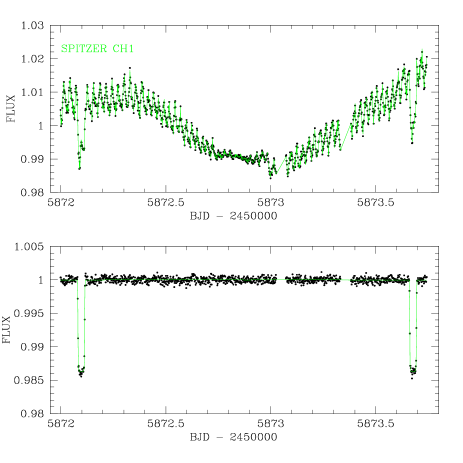
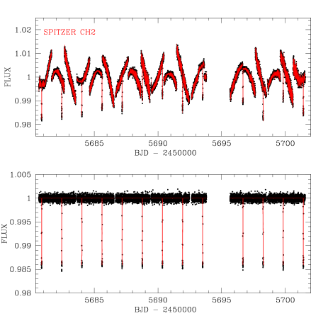
Figure 2: $Top$: 3.6 $\mu$m ($left$) and 4.5 $\mu$m ($right$) light curves obtained in our program 70049 for GJ 1214, with the best-fit global models (Sect. 3.2) for each AOR superimposed. $Bottom$: The same after division by the best-fit instrumental models.

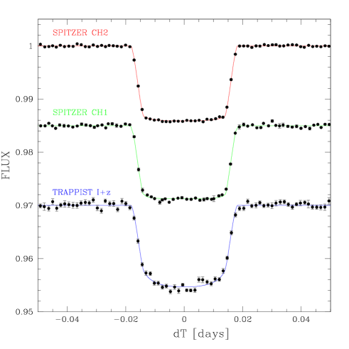
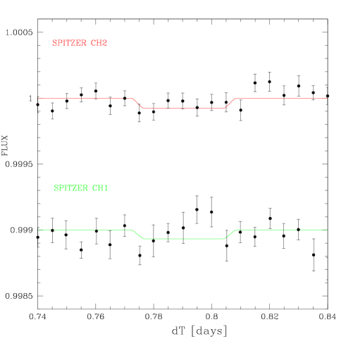
Figure 3: Detrended photometry period-folded on the best-fit transit ephemeris obtained in our global analysis (Sect. 3.2) after zoom on the transit ($left$) and occultation ($right$) phases. For the transit and occultation phases, the measurements were binned per interval of 2 min and 7.2 min, respectively. For both panels, the best-fit eclipse models are superimposed.

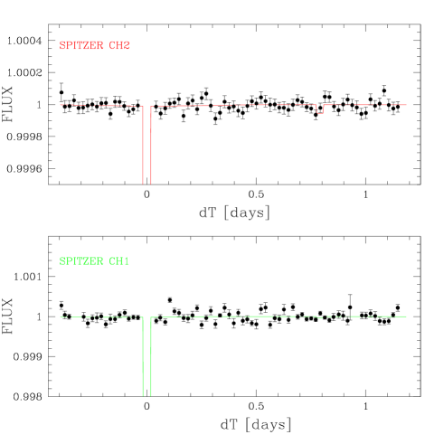
Figure 4: Detrended Spitzer 3.6 $\mu$m ($top$) and 4.5 $\mu$m ($bottom$) photometry folded on the best-fit transit ephemeris obtained in our global analysis (Sect. 3.2), binned per intervals of 30 min. The best-fit eclipse + phase-curve models are superimposed.

3.3 Analysis assuming an eccentric orbit

As outlined by Carter et al. (2011), the circularization timescale of GJ 1214 b could be as long as 10 Gyr for specific compositions, while several transiting Neptune-like planets have significantly eccentric orbits. Even when considering the new HARPS measurements, a small orbital eccentricity is still possible, so based on these considerations it is desirable to assess the influence of the circular orbit assumption on the stellar and planetary size, and on the planet’s thermal emission. To carry out this task, we performed a second MCMC analysis with the orbital eccentricity $e$ and argument of pericenter $\omega$ free, the corresponding jump parameters being $\sqrt{e}\cos\omega$ and $\sqrt{e}\sin\omega$. Gaussian prior probability distributions were assumed for these two jump parameters, based on the values $\sqrt{e}\cos\omega=0\pm 0.12$ and $\sqrt{e}\sin\omega=-0.10\pm 0.17$ deduced from the analysis of the new HARPS dataset. The corresponding distributions for $e\cos\omega$ and $e\sin\omega$ are, respectively, $0.00\pm 0.02$ and $-0.02_{-0.06}^{+0.03}$.

The results of this second analysis are given in Table 3 (MCMC 2). It can be seen that the derived parameters for the system are in good agreement with the ones deduced under the circular orbit assumption, but some are less precise because the uncertainties on $e$ and $\omega$ propagate to the parameters $a/R_{\ast}$, $\rho_{\ast}$, $R_{\ast}$, and $R_{p}$. We note, however, that our adopted results are the ones from the analysis assuming a circular orbit, based on the absence of observational evidence for a significant eccentricity ($\Delta$BIC = -20 in favor of the circular model).

3.4 Analysis with a uniform prior distribution on the limb-darkening coefficients

We explored the influence of our selected priors on the limb-darkening by performing a MCMC analysis assuming for all channels uniform prior distributions on the quadratic limb-darkening coefficients $u_{1}$ and $u_{2}$. Its results are presented in Table 3 (MCMC 3). While some derived values are slightly less precise than the ones obtained in our adopted analysis, they are in excellent agreement ($<1\sigma$) with them, including for the parameters defining the transit shape ($dF$, $b^{\prime}$, $W$, $\rho_{\ast}$, $a/R_{\ast}$, $i$). We thus conclude that the results of our adopted analysis are not influenced by our selected priors on the limb-darkening coefficients.

3.5 Analysis allowing for transit timing variations

In a final MCMC analysis, we let the timings of the transits present in our Spitzer + TRAPPIST dataset be jump parameters. Our goal was to benefit from the strong constraints brought by the global analysis on the transit shape and depth to reach the highest possible sensitivity on possible transit timing variations (TTVs, Holman & Murray 2005, Agol et al. 2005) due to another unknown object in the system. In this analysis, we assumed a circular orbit for GJ 1214 b, and normal prior distributions based on the results of our adopted analysis (Table 3, MCMC 1) for the jump parameters $P$ and $T_{0}$.

Table 4 presents the derived transit timings. A linear regression using these timings and their epochs as input led to the following transit ephemeris: $2454980.748996(\pm 0.000084)+N\times 1.58040418(\pm 0.00000019)$ BJD_TDB, $N$ being the epoch. This ephemeris agrees well with the MCMC result (Table 3).

Figure 5 shows the resulting TTVs as a function of the epochs of the transits. As can be seen in this figure, we could not detect any significant TTV, which is consistent with the results that we independently obtained in F13 from the same data.

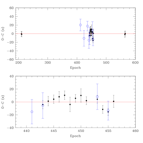
Figure 5: $Top$: transit timing variations deduced from our global analysis for the Spitzer and TRAPPIST transits (see Sec. 3.4). $Bottom$: zoom on the consecutive transits observed by Spitzer in April and May 2011. Three of these transits were also observed by TRAPPIST.

	MCMC 1	MCMC 2	MCMC 3
	$e=0$	$e\geq 0$	$e=0$, LD free
Jump parameters
$M_{\ast}$ [$M_{\odot}$]	$0.176\pm 0.009$ $(p)$	$0.176\pm 0.009$ $(p)$	$0.176\pm 0.009$ $(p)$
$T_{eff}$ [K]	$3250\pm 100$ $(p)$	$3250\pm 100$ $(p)$	$3250\pm 100$ $(p)$
$[Fe/H]$ [dex]	$0.1\pm 0.1$ $(p)$	$0.1\pm 0.1$ $(p)$	$0.1\pm 0.1$ $(p)$
$dF_{3.6\mu m}$ [%]	$1.3545\pm 0.0085$	$1.3521\pm 0.0083$	$1.342\pm 0.015$
$dF_{4.5\mu m}$ [%]	$1.3676\pm 0.0039$	$1.3673\pm 0.0039$	$1.365\pm 0.011$
$dF_{I+z}$ [%]	$1.377\pm 0.020$	$1.376\pm 0.021$	$1.385\pm 0.026$
$dF_{occ,3.6\mu m}$ [ppm]	$45_{-30}^{+44}$	$74_{-51}^{+96}$	$44_{-29}^{+44}$
	$<205$ (99.7% confidence)	$<585$ (99.7% confidence)	$<184$ (99.7% confidence)
$dF_{occ,4.5\mu m}$ [ppm]	$70\pm 35$	$37_{-28}^{+41}$	$67\pm 35$
	$<190$ (99.7% confidence)	$<158$ (99.7% confidence)	$<177$ (99.7% confidence)
$A_{3.6\mu m}$ [ppm]	$11_{-8}^{+15}$	$16_{-12}^{+27}$	$11_{-8}^{+16}$
	$<68$ (99.7% confidence)	$<166$ (99.7% confidence)	$<78$ (99.7% confidence)
$O_{3.6\mu m}$ [deg]	$350_{-110}^{+120}$	$10_{-130}^{+100}$	$0_{-110}^{+120}$
$A_{4.5\mu m}$ [ppm]	$16_{-12}^{+18}$	$11_{-8}^{+16}$	$18_{-13}^{+18}$
	$<68$ (99.7% confidence)	$<68$ (99.7% confidence)	$<73$ (99.7% confidence)
$O_{4.5\mu m}$ [deg]	$325_{-110}^{+160}$	$335_{-110}^{+170}$	$320_{-110}^{+180}$
$b^{\prime}$ [$R_{\ast}$]	$0.385\pm 0.022$	$0.371_{-0.030}^{+0.017}$	$0.367\pm 0.032$
$W$ [min]	$52.52\pm 0.14$	$52.52\pm 0.13$	$52.45\pm 0.15$
$T_{0}$ [BJDTDB]	$2454980.74900\pm 0.00010$	$2454980.74901\pm 0.00010$	$2454980.74898\pm 0.00008$
$P$ [d]	$1.58040417\pm 0.00000022$	$1.58040415\pm 0.00000020$	$1.58040421\pm 0.00000018$
$\sqrt{e}\cos\omega$	0 (fixed)	$-0.05\pm 0.10$	0 (fixed)
$\sqrt{e}\sin\omega$	0 (fixed)	$-0.13\pm 0.21$	0 (fixed)
$c_{1}(3.6{\mu}m)$	$0.143\pm 0.010$	$0.143\pm 0.010$	$0.204_{-0.087}^{+0.082}$
$c_{2}(3.6{\mu}m)$	$-0.392\pm 0.010$	$-0.391\pm 0.010$	$-0.77\pm 0.54$
$c_{1}(4.5{\mu}m)$	$0.189\pm 0.010$	$0.189\pm 0.010$	$0.258\pm 0.039$
$c_{2}(4.5{\mu}m)$	$-0.3999\pm 0.0070$	$-0.3995\pm 0.0070$	$-0.12_{-0.47}^{+0.34}$
$c_{1}(I+z)$	$0.749\pm 0.063$	$0.753\pm 0.068$	$0.87\pm 0.11$
$c_{2}(I+z)$	$-0.53\pm 0.14$	$-0.54\pm 0.15$	$0.45_{-0.66}^{+0.63}$
Stellar parameters
$R_{\ast}$ [$R_{\odot}$]	$0.2213\pm 0.0043$	$0.217_{-0.015}^{+0.010}$	$0.2198\pm 0.0045$
Luminosity $L_{\ast}$ [$R_{\odot}$]	$0.00488_{-0.00060}^{+0.00068}$	$0.00465_{-0.00079}^{+0.00082}$	$0.00484_{-0.00059}^{+0.00064}$
Density $\rho_{\ast}$ [$\rho_{\odot}$]	$16.25\pm 0.46$	$17.1_{-1.6}^{+3.9}$	$16.53\pm 0.57$
Surface gravity $\log{g}_{\ast}$ [cgs]	$4.994\pm 0.012$	$5.010_{-0.035}^{+0.061}$	$4.999\pm 0.014$
$u_{1}(3.6{\mu}m)$	$-0.0210\pm 0.0052$ $(p)$	$-0.0209\pm 0.0053$ $(p)$	$-0.08_{-0.11}^{+0.14}$
$u_{2}(3.6{\mu}m)$	$0.1852\pm 0.0050$ $(p)$	$0.1852\pm 0.0045$ $(p)$	$0.34_{-0.20}^{+0.22}$
$u_{1}(4.5{\mu}m)$	$-0.0046\pm 0.0050$ $(p)$	$-0.0044\pm 0.0048$ $(p)$	$0.08_{-0.10}^{+0.08}$
$u_{2}(4.5{\mu}m)$	$0.1976\pm 0.0030$ $(p)$	$0.1975\pm 0.0029$ $(p)$	$0.10_{-0.13}^{+0.19}$
$u_{1}(I+z)$	$0.193\pm 0.049$ $(p)$	$0.194\pm 0.049$ $(p)$	$0.44_{-0.17}^{+0.16}$
$u_{2}(I+z)$	$0.363\pm 0.063$ $(p)$	$0.366\pm 0.060$ $(p)$	$0\pm 0.26$
Planet parameters
$(R_{p}/R_{\ast})_{3.6\mu m}$	$0.11638\pm 0.00037$	$0.11638\pm 0.00035$	$0.11587_{-0.00067}^{+0.00058}$
$(R_{p}/R_{\ast})_{4.5\mu m}$	$0.11694\pm 0.00017$	$0.11693\pm 0.00017$	$0.11685_{-0.00052}^{+0.00043}$
$(R_{p}/R_{\ast})_{I+z}$	$0.11735\pm 0.00086$	$0.11732\pm 0.00090$	$0.1177\pm 0.0011$
$a/R_{\ast}$	$14.45\pm 0.15$	$14.7_{-0.5}^{+1.0}$	$14.54_{-0.16}^{+0.18}$
$a$ [au]	$0.01488\pm 0.00025$	$0.01489\pm 0.00025$	$0.01486\pm 0.00025$
$i$ [deg]	$88.47\pm 0.10$	$88.56_{-0.16}^{+0.18}$	$88.55\pm 0.14$
$e$	0 (fixed)	$0.054_{-0.044}^{+0.087}$	0 (fixed)
$\omega$ [deg]	-	$249_{-100}^{+47}$	-
$e\cos\omega$	0 (fixed)	$-0.007_{-0.023}^{+0.032}$	0 (fixed)
$e\sin\omega$	0 (fixed)	$-0.026_{-0.065}^{+0.035}$	0 (fixed)
$T_{eq}$ [K]a	$604\pm 19$	$596_{-26}^{+24}$	$603\pm 19$
$R_{p,3.6\mu m}$ [$R_{\oplus}$]	$2.805\pm 0.056$	$2.75_{-0.19}^{+0.11}$	$2.776\pm 0.061$
$R_{p,4.5\mu m}$ [$R_{\oplus}$]	$2.821\pm 0.056$	$2.77_{-0.19}^{+0.11}$	$2.799\pm 0.061$
$R_{p,I+z}$ [$R_{\oplus}$]	$2.830\pm 0.062$	$2.78_{-0.19}^{+0.12}$	$2.823\pm 0.069$

Table 3: Median and 1-$\sigma$ limits of the marginalized a posteriori probability distributions for the jump and system parameters from our global MCMC analysis of Spitzer and TRAPPIST photometry (Sect. 3). The analysis we adopted is MCMC 1. $(p)$: a normal prior distribution was assumed (see text for details). ^aAssuming a null Bond albedo and a homogeneous heat distribution between both hemispheres.

Observatory	Channel	Epocha	Mid-transit time
			($BJD_{TDB}$)
Spitzer	$S1$	210	$5312.633866\pm 0.000069$
Spitzer	$S2$	211	$5314.214261\pm 0.000069$
TRAPPIST	$I+z$	412	$5631.87575\pm 0.00016$
TRAPPIST	$I+z$	424	$5650.84024\pm 0.00021$
TRAPPIST	$I+z$	436	$5669.80542\pm 0.00013$
TRAPPIST	$I+z$	441	$5677.70706\pm 0.00022$
Spitzer	$S2$	443	$5680.867997\pm 0.000074$
TRAPPIST	$I+z$	443	$5680.86798\pm 0.00023$
Spitzer	$S2$	444	$5682.448463\pm 0.000085$
Spitzer	$S2$	445	$5684.028902\pm 0.000076$
Spitzer	$S2$	446	$5685.609349\pm 0.000095$
Spitzer	$S2$	447	$5687.189781\pm 0.000077$
Spitzer	$S2$	448	$5688.77002\pm 0.00013$
Spitzer	$S2$	449	$5690.350535\pm 0.000070$
Spitzer	$S2$	450	$5691.93099\pm 0.00012$
Spitzer	$S2$	451	$5693.511301\pm 0.000071$
Spitzer	$S2$	453	$5696.672135\pm 0.000069$
TRAPPIST	$I+z$	453	$5696.67218\pm 0.00023$
Spitzer	$S2$	454	$5698.252357\pm 0.000071$
Spitzer	$S2$	455	$5699.832716\pm 0.000064$
TRAPPIST	$I+z$	455	$5699.83274\pm 0.00017$
Spitzer	$S2$	456	$5701.41331\pm 0.00011$
Spitzer	$S1$	564	$5872.096930\pm 0.000085$
Spitzer	$S1$	565	$5873.677356\pm 0.000072$

Table 4: Transit mid-times and 1$\sigma$ errors for the Spitzer and TRAPPIST transits from our global analysis (Sect. 3.4). $S1$ and $S2$ denote, respectively, the 3.6 $\mu$m and 4.5 $\mu$m channels of Spitzer/IRAC. ^aThe epoch is relative to the transit ephemeris shown in Table 3.

4 Search for a second transiting planet

We used the best-fit residuals Spitzer light curve obtained from our adopted global analysis to perform a search for the transit(s) of a possible second planet. We did not use the TRAPPIST residuals as their photometric precision is significantly weaker. Our residuals light curve contains 14,293 photometric measurements. For each measurement, the error bar was multiplied by the corresponding $\beta_{w}$ factor (see Table 1) to take into account the actual white noise budget of the data. For each of the three channels, we also multiplied the error bars by the mean $\beta_{r}$ for this channel. We did not use for each light curve its derived $\beta_{r}$ shown in Table 1, as a larger $\beta_{r}$ could be due to a transit.

Our procedure was based on a search for periodic transit-like signals over a grid of periods, phases, impact parameters, and depths. The probed periods ranged from 0.1day to 20.9 days, the period step being 0.0001days (8.6 s). For each period step, transit models centered at 100 evenly separated phases were compared to the period-folded light curve, assuming a circular orbit, $M_{\ast}=0.176$ $M_{\odot}$, and $R_{\ast}=0.221$ $R_{\odot}$. For each phase, transit models with impact parameters of 0 and 0.5, and depths ranging from 100 ppm to 1000 ppm, were tested. For each period, the chi-square $\chi^{2}$ corresponding to the best-fitting transit profile in terms of phase, depth, and impact parameter was registered and compared to the chi-square assuming no transit.

Figure 6 presents the resulting transit periodogram. The strongest power peak corresponds to $P$=0.4157 days, the improvement of the $\chi^{2}$ being 15.8. The corresponding folded light curve is also shown in Fig. 6. With 14293 measurements and 4 more degrees of freedom for the transit model, a $\Delta\chi^{2}=-15.8$ corresponds to a $\Delta BIC=-15.8+4\log(14293)=+22.5$. Using the BIC as a proxy for the model marginal likelihood, this $\Delta BIC$ results in a Bayes factor of $e^{\Delta BIC/2}=77000$ in favor of the no-transit model, translating into a false alarm probability (FAP) of $\sim$99.999%. This power peak in the periodogram has not yet represented a significant signal. A simple computation shows that a $\chi^{2}$ improvement of $\sim$ -50 would be required to result in a transit model one hundred times more likely than the no-transit model (FAP $\sim$ 1 %).

To better investigate the significance of the highest peak of our transit periodogram, we performed two MCMC global analyses similar to the ones described in Sect. 3, each composed of two chains of 100,000 steps. The first MCMC model included only GJ 1214 b, assuming for it a circular orbit, no TTV, no transit depth chromaticity, no phase curve, and no occultation. In the second MCMC, we added a second transit planet in circular orbit with $P\sim 0.4157$ day. From the two resulting BICs, a Bayes factor was again computed. The advantage of this procedure is that it does not use the best-fit residual light curves for which a shallow transit signal could have been partially erased by the baselines detrending. Furthermore, all the free parameters of the models have their a posteriori probability distributions probed in the same process, ensuring a proper error propagation. Compared to the model without a second transiting planet, the two-planet model is shown to be $\sim$650 times less likely, confirming thus that the strongest peak in the periodogram shown in Fig. 6 does not correspond to a significant transit signal.

To ensure that no periodic transit-like signal was missed by our algorithm, we also analyzed our Spitzer residuals light curve with the BLS algorithm (Kovács et al. 2002) available on the NASA Exoplanet Archive website. Here, BLS found several power excesses at short periods, the most significant corresponding to 2.2025 days, its derived false alarm probability (FAP) being $\sim 1$ %. Once folded with this period, the residuals light curve shows a tiny transit-like signal with an amplitude of $\sim$ 100 ppm (Fig. 7). Still, its duration is $\sim$ 5 hr, which is $\sim$ 5 times longer than expected for the central transit of a planet in a 2.2-day circular orbit around GJ 1214. This explains why our transit search algorithm did not detect this possible signal. Nevertheless, we decided to better assess its reality by performing the same MCMC procedure described above. Here too, the result is that the putative transit signal is not significant, the resulting Bayes factor being $10^{24}$ in favor of the model without a second transiting planet.

We also noticed that several among the strongest BLS peaks corresponded to flux increases instead of drops, suggesting that the forest of peaks at short periods is due to red noise of instrumental or astrophysical origin. From the injection of simulated periodic transits of different periods and depths in the raw photometry and their analysis using the same procedure as described above (global modeling GJ 1214 b + systematics, transit search in the resulting residuals, short MCMC for the most significant detected signals), we concluded that only transits deeper than $\sim 200$ ppm (for periods $<$1 day) to $\sim 500$ ppm (for unique transits) could be firmly detected in our Spitzer GJ 1214 data; this limitation comes from the combination of the photon noise ($\sim 90$ ppm per hour) and the $50-100$ ppm red noise present in the light curves. These limits correspond to a range in planetary radii of 0.35 - 0.5 $R_{\oplus}$.

For the sake of completeness, we also performed a visual search for transit-like structures in the residual light curves, but failed to detect anything convincing. We thus conclude that there is an absence of evidence for a second transiting planet around GJ 1214 in the Warm Spitzer photometry, while we would have clearly detected any transit of a Mars-size or larger planet.

Figure 6: $Top$: Transit search periodogram obtained from the analysis of the photometric residuals (Sect. 4). $Bottom$: Spitzer residuals folded on the ephemeris of the most significant transit signal found by our transit search algorithm ($P$=0.4157 day), and binned per intervals of 15 mins.

Figure 7: $Top$: BLS periodogram obtained from the analysis of the Spitzer residuals light curve (Sect. 4). $Bottom$: Spitzer residuals folded on the ephemeris of the most significant transit signal found by the BLS algorithm ($P$=2.2025 days), and binned per intervals of 30 mins.

5 Discussion

5.1 The accuracy of our derived parameters

The values deduced in our adopted analysis (MCMC 1 in Table 2) for the physical parameters $a/R_{*}$ and $i$ that define the transit shape (see, e.g., Winn 2011) are in good agreement with the values reported in the GJ 1214 b detection paper (C09), but disagree with several values reported afterwards and based on high-precision photometry from the ground (Berta et al. 2011) or from space (Berta et al. 2012). Notably, the agreement with our own results presented in F13 is rather poor, while both analyses were based on the same dataset. This is illustrated in Fig. 8 ($left$). This figure shows a clear correlation between $a/R_{*}$ (and thus the stellar density) and the orbital inclination $i$. The simplest explanation to this correlation is that some of the shown measurements are affected by systematic errors. For a given orbital period, the same transit duration can be obtained from a larger star combined with a smaller inclination, leading to a degeneracy between $a/R_{*}$ and $i$ that can be broken only by a very accurate determination of the transit shape. This is generally a difficult exercise because the red noise of the photometric time-series and the limb-darkening profile of the star alter the original trapezoidal profile of the transit. Depending on the data quality and the details of the analysis, the derived values for $a/R_{*}$ and $i$ can easily be affected by small systematic errors that are difficult to identify. In F13, we recognized the possibility of systematic errors in our analysis of the Spitzer data, so we forcibly varied $a/R_{*}$ to evaluate the effect on $R_{p}/R_{*}$ (which was the most important parameter for that analysis). These systematics in F13 could be due to the two-step approach used in our analysis that started with the decorrelation of the raw photometry followed by the analysis of the detrended light curves. This strategy is not the best one to use for an accurate determination of transit parameters, as the initial decorrelation phase can slightly distort the transit shape and represents a source of error that is not explicitly propagated to the fitted transit parameters. The strategy used here that consists in the global modeling of the planetary and instrumental signals is better able to accurately determine the transit parameters. Nevertheless, we note that our main goal in F13 was the accurate measurement of the transmission spectrum of the planet. This goal was clearly achieved, as demonstrated not only by the agreement between the transit depths measured in F13 for each channel with three different methods, but also by their excellent agreement with our independent measurements presented here (see Table 6).

Our multi-band global analysis strategy should be the best choice for breaking the degeneracy between $a/R_{*}$ and $i$, notably by averaging the influence of the instrumental systematics present in the different channels and by minimizing the impact of the limb-darkening uncertainties and the assumed model. Notably, this is supported by the results of our MCMC 3 analysis that did not assume any prior distribution on the limb-darkening coefficients and still led to system parameters in excellent agreement ($<1-\sigma$) with the ones derived in our adopted MCMC 1 analysis (see Table 2). To test further the reliability of our derived parameters, for the three channels probed by our data we modeled the transits of a 2.8 $R_{\oplus}$ planet in front of a 0.176 $M_{\odot}$ - 0.221 $R_{\odot}$ star, assuming an orbital period and inclination of $P$=1.58040417 d and $i=88.5^{\circ}$, respectively, and quadratic limb-darkening coefficients drawn from the Claret & Bloemen (2011) tables for $T_{eff}=3250$ K, $\log{g}=5.0$, and [Fe/H] = $0.1$. We injected the corresponding transit profiles into our original light curves after dividing them by the best-fit transit models selected by our MCMC 1 analysis. We then performed a new MCMC analysis similar to MCMC 1 in every way that resulted in parameter values fully consistent with the ones of MCMC 1. Notably, we obtained $a/R_{\ast}=14.52\pm 0.15$ and $i=88.44\pm 0.10$ deg, in excellent agreement ($<1\sigma$) with our input values. This test suggests that our results for the transit shape parameters are accurate and do not suffer from strong systematic errors related to the details of our data analysis.

An actual chromatic variability of the transit shape could also explain the pattern visible in Fig. 8. It could be due to an inhomogeneous opacity of the planet limb at transit. To test this hypothesis, we performed separate MCMC analyses of the Spitzer 3.6 $\mu$m, 4.5 $\mu$m, and TRAPPIST $I+z$ photometry. The results are shown in Fig. 8 ($right$) and in Table 5. The parameters derived for the three channels are in excellent agreement with each other and with the results of our global MCMC 1 analysis. From this consistency, we conclude that systematic errors are the most plausible explanation for the correlation between the measurements for $a/R_{*}$ and $i$ shown in Fig. 8 ($left$).

	$I+z$	3.6 $\mu$m	4.5 $\mu$m
$a/R_{\ast}$	$14.64_{-0.67}^{+0.76}$	$14.62_{-0.33}^{+0.35}$	$14.48_{-0.15}^{+0.17}$
$i$ [deg]	$88.76_{-0.52}^{+0.70}$	$88.57_{-0.23}^{+0.28}$	$88.50\pm 0.12$
$R_{p}/R_{\ast}$	$0.1160\pm 0.0017$	$0.11629\pm 0.00040$	$0.11688\pm 0.00018$

Table 5: Median and 1-$\sigma$ limits of the marginalized a posteriori probability distributions for the parameters $a/R_{\ast}$, $i$, and $R_{p}/R_{\ast}$ derived from the separate analyses of the Spitzer 3.6 $\mu$m, 4.5 $\mu$m, and TRAPPIST $I+z$ photometry (Sect. 5.1).

	This work	F13a	F13b	F13c
$(R_{p}/R_{\ast})_{I+z}$	$0.11735\pm 0.00086$	$0.1187\pm 0.0011$	$0.1179\pm 0.0018$	$0.11803\pm 0.00079$
$(R_{p}/R_{\ast})_{3.6\mu m}$	$0.11638\pm 0.00037$	$0.11607\pm 0.00030$	$0.11616\pm 0.00019$	$0.11602\pm 0.00055$
$(R_{p}/R_{\ast})_{4.5\mu m}$	$0.11694\pm 0.00017$	$0.11710\pm 0.00017$	$0.11699\pm 0.00026$	$0.11709\pm 0.00022$

Table 6: Comparison of the planet-to-star radius ratio derived in this work and in F13 from the same data. F13a = simultaneous analysis for each channel; F13b = average of the results of individual analyses for each channel; F13c = analysis of the phase & binned light curve for each channel.

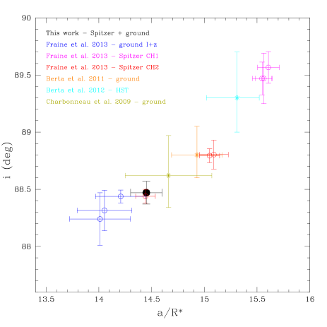
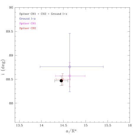
Figure 8: Diagram of orbital inclination $i$ $vs.$ $a/R_{\ast}$ scale ratio. Our measurement is shown as a filled black circle. $Left$: comparison with the measurements presented by F13, C09 (ground), Berta et al. (2011) (ground), and Berta et al. (2012) (HST). $Right$: comparison of our measurement obtained from the global analysis of Spitzer and TRAPPIST data to the measurements that we obtained from separate analyses of the Spitzer 3.6 $\mu$m, 4.5 $\mu$m, and TRAPPIST data alone.

5.2 The presence of a habitable planet transiting GJ 1214

The main motivation for our ambitious Spitzer program was to explore the HZ of GJ 1214 in search of a transiting planet, with a sensitivity high enough to detect any Mars-sized or larger planet. In practice, we did not probe the whole HZ, as new estimates of its limits by Kopparapu et al. (2013) predict an outer edge of 0.13 au for GJ 1214, corresponding to a period of 44 days. In full generality, probing the entire HZ is in fact impossible, as the actual HZ outer limit depends strongly on atmospheric composition (e.g., planets with hydrogen-dominated atmospheres could be habitable out to 1-2 au, Pierrehumbert & Gaidos 2011), and possibly on the internal heat of the planets (Stevenson 1999). We thus probed only the inner part of the HZ, defined here as $P<20.9$ d.

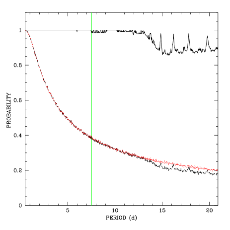
Figure 9: Black solid line: probability for the transit of a second putative planet occurring at least once during the Spitzer observations as a function of the orbital period, for periods up to 20.9 d. Black dots: transit probability for a second planet, taking into account the transiting nature of GJ 1214 b (see Sect. 5.2 for details). The red line shows the product of the two probabilities. The green vertical line shows the inner limit of the HZ as computed from eq. 12 of Zsom et al. (2013).

We were able to reach the desired sensitivity, but unfortunately we did not detect a second planet transiting the red dwarf. Because we could not continuously monitor GJ 1214 during the 20.9 days, there is a small chance that we missed the transit of a second planet orbiting in the inner part of the HZ, especially if it is a planet with a longer period. To estimate this probability as a function of the orbital period, we used the timings of the Spitzer data and determined for each orbital period the fraction of orbital phases for which a mid-latitude transit would have happened at least once inside our observation window. The resulting probabilities are shown in Fig. 9. For the inner part of the HZ, the mean probability to have observed at least one transit is 94%, meaning that there is a 6% chance that we missed the transit(s). So we cannot firmly reject (at 3-$\sigma$ or better) that we missed the transit of a planet orbiting in the inner part of the HZ, but the corresponding probability is certainly too low to justify additional monitoring of the system with a space telescope. For orbits closer than the HZ ($P<7.5$ d, using eq. 12 of Zsom et al. 2013 and our derived stellar luminosity $\sim 0.0049$ $L_{\odot}$), the mean probability to have observed at least one transit is 99.999%, so we can firmly reject the presence of a second Mars-sized transiting planet for orbits closer than the HZ.

Using a similar Monte-Carlo simulation procedure to the one described in G11, we derived the transit probability for a putative second planet taking into account the transiting nature of GJ 1214 b, using our new derived parameters for the stellar size and for the orbital inclination of GJ 1214 b, and drawing values out of the normal distribution $N(0,2.2^{2})$ deg for the difference in inclination between both planets, 2.2 deg being the $rms$ of the inclinations of the solar system planets. This value is consistent with the spread in inclinations observed for Kepler multi-planetary systems (Fabrycky et al. 2012). The resulting probabilities are presented in Fig. 9 as a function of the orbital periods. The mean value for the inner part of the HZ is 27%, and 61% for the zone closer than the HZ. Multiplying this geometric probability by the window probability derived above, and averaging for the whole inner part of the HZ, we estimate that our a priori chance of success of detecting a habitable planet of Mars-size or above was 25%, assuming GJ 1214 does harbor such a planet with $P<20.9$ d. Under this assumption, and taking into account our non-detection, the a posteriori probability that the planet does not transit is $\sim 98$%, while the a posteriori probability that it does transit and that we missed its transit is thus $\sim 2$%.

5.3 The atmospheric properties of GJ 1214 b

The atmosphere of GJ 1214 b has been the subject of intense scrutiny in the recent past. Previous studies of the atmosphere of GJ 1214 b have been based on observations of transmission spectra, which probe the regions near the day-night terminator of the planet. The sum total of existing data with multiple instruments over a wide spectral baseline ($\sim 0.8-5\mu$m) indicate a flat transmission spectrum (Bean et al. 2010 & 2011; Désert et al. 2011; Berta et al. 2011; de Mooij et al. 2012 & 2013; Teske et al. 2013; but cf Croll et al. 2011). This spectrum is indicative of either a cloudy atmosphere with unknown composition (potentially H₂-rich) or an atmosphere with a high mean molecular weight ($\mu$), for example, an H₂O-rich atmosphere (Bean et al. 2010; Désert et al. 2011; Kempton et al. 2012; Benneke & Seager 2012; Howe & Burrows 2012; Morley et al. 2013). Constraining the atmospheric $\mu$ of GJ 1214 b is important to address the fundamental question of whether super-Earths represent scaled-down Neptunes or scaled-up terrestrial planets. While a cloudy H₂-rich atmosphere would indicate a Neptune-like atmosphere for the planet, a high-$\mu$ atmosphere would suggest a terrestrial-like atmosphere. Current observations of the planetary atmosphere are unable to break the degeneracy between the two scenarios and so are inconclusive regarding the true composition of GJ 1214 b.

Our observations of the secondary eclipses of GJ 1214b place constraints on the dayside atmosphere of the planet, a region not accessible to transmission observations. We use two photometric observations of the planet-star flux ratios in the 3.6 $\mu$m and 4.5 $\mu$m bandpasses of Spitzer. We model the planetary thermal emission at secondary eclipse using the exoplanetary atmospheres modeling and retrieval method of Madhusudhan & Seager (2009). The model computes line-by-line radiative transfer in a 1D plane-parallel atmosphere, with constraints of local thermodynamic equilibrium, hydrostatic equilibrium, and global energy balance. The pressure-temperature ($P-T$) profile and the molecular composition are free parameters of the model, allowing exploration of models with a wide range of temperature profiles (e.g., with and without temperature inversions) and chemical compositions (varied $\mu$, C/O ratios, etc.). However, given that we have only two photometric data points, compared to $\sim$10 free parameters depending on the specific model in question, the model space is presently under-constrained. We, therefore, consider canonical models of the dayside atmosphere of GJ 1214 b and investigate their potential in explaining the current data. We consider (1) H₂-rich solar composition models, (2) H₂O-rich models (called water worlds), and (3) cloudy models parametrized by an optically thick cloud deck at a parametric pressure level.

Our results rule out a cloud-free solar abundance H₂-rich composition in the dayside atmosphere of GJ 1214 b. In the temperature regime of GJ 1214 b, as shown in the inset in Fig. 10, a solar abundance composition in chemical equilibrium predicts methane (CH₄) and water vapor (H₂O) to be the most dominant molecules bearing carbon and oxygen, respectively; CO₂ to be present at the $\sim$1 ppm level; and CO to be negligible (Madhusudhan & Seager 2011; Madhusudhan 2012). The molecules CH₄ and H₂O have strong absorption in the 3.6 $\mu$m Spitzer channel, whereas CO and CO₂ have strong absorption features in the 4.5 $\mu$m Spitzer channel. Therefore, given their relative abundances, the corresponding model spectrum shows strong absorption in the 3.6 $\mu$m Spitzer channel and less absorption in the 4.5 $\mu$m channel, as shown in Fig 10. While this model spectrum explains the low planet-star flux contrast observed in the 3.6 $\mu$m, it predicts significantly higher contrast than is observed in the 4.5 $\mu$m channel.

On the other hand, our observations are consistent with both a metal-rich atmosphere and a cloudy H₂-rich atmosphere. Model atmospheres with a wide range of metal-rich compositions can explain the data. As shown in Fig 10, a water-world atmosphere (e.g., Miller-Ricci et al. 2009), with 99% water vapor by volume fits both data within the 1-$\sigma$ uncertainties. The high mean-molecular weight of such an atmosphere causes a short atmospheric scale height, which together with the strong absorption features of water vapor cause low planet-star flux ratios across the near- to mid-infrared spectrum. This spectrum is consistent with the low planet-star flux ratios we observe in both the Spitzer channels at 3.6 $\mu$m and 4.5 $\mu$m. We also find that both the photometric data are consistent with a featureless blackbody spectrum of the planet with a temperature of $\sim$500-600 K, similar to a H₂-rich atmosphere with a gray-opacity cloud deck at pressures below $\sim$50 mbar. In this regard, our constraints on the composition of the dayside atmosphere of GJ 1214b are similar to the constraints on the atmospheric composition at the day-night terminator of the planet obtained from transmission spectra in the recent past (e.g., Bean et al. 2010, 2011; Désert et al. 2011; Berta et al. 2012).

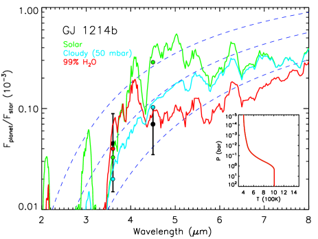
Figure 10: Observations and model spectra of thermal emission from GJ 1214b. The black circles with error bars show the planet-star flux ratios observed in the Spitzer IRAC bandpasses at 3.6 $\mu$m and 4.5 $\mu$m. The green and red solid curves in the main panel show model spectra of an atmosphere with a solar abundance H₂-rich composition and one with a water-rich composition, respectively. The inset shows the temperature profiles for both models. The blue dashed curves show blackbody spectra of the planet with temperatures of 500 K, 600 K, and 700 K.

6 Conclusions

In G11, we had identified GJ 1214 as a high-priority target for a transit search, as a habitable planet orbiting this nearby M4.5 dwarf should have its transit probability strongly enhanced by the transiting nature of GJ 1214 b. In this context, we set up an ambitious high-precision photometric monitoring of GJ 1214 with the Spitzer Space Telescope to probe the inner part of its HZ ($P<20.9$ d) in search of a planet as small as Mars. Because of a DNS failure, we could not probe the entire inner HZ, but still we covered about 94% of it.

After having presented in a first paper (F13) our detailed study of the Spitzer transits of GJ 1214 b, and its implications for the transmission spectrum of the planet, we have reported here the results of our transit search and of our global analysis of a very extensive photometric dataset combining all the Spitzer data acquired for GJ 1214 to new ground-based transit light curves. Unfortunately, we did not detect a second transiting planet. Assuming that GJ 1214 hosts a habitable planet larger than Mars and with $P<20.9$ d, our global analysis of the whole Spitzer dataset leads to an a posteriori no-transit probability $\sim 98$%. Still, our analysis allowed us to significantly improve the characterization of GJ 1214 b, notably by detecting at 2-$\sigma$ its 4.5 $\mu$m thermal emission, and by constraining its 3.6 $\mu$m occultation depth to be smaller than 205ppm (3-$\sigma$ upper limit). These emission measurements is new empirical evidence against a cloud-free hydrogen-rich atmosphere for this intriguing super-Earth.

- (1) Anglada-Escudé, G., Rojas-Ayala, B., Boss, A. P., et al., 2013, A&A, 551, A48
- (2) Agol, E., Steffen, J., Sari, R., & Clarkson W., 2005, MNRAS, 359, 567
- (3) Bean, J. L., Miller-Ricci Kempton, E., & Derek, H. 2010, Nature, 468, 669
- (4) Bean, J. L., Désert, J.-M., Kabath, P., et al., 2011, ApJ, 743, 92
- (5) Benneke, B. & Seager S. 2012, ApJ, 753, 100
- (6) Berta, Z. K., Charbonneau, D., Bean, J., et al. 2011, ApJ, 736, 12
- (7) Berta, Z.K., Charbonneau, D., Désert J.-M., et al. 2012, ApJ, 747, 35
- (8) Carter, J. A., Winn, J. N., Holman, M. J., et al. 2011, ApJ, 730, 82
- (9) Charbonneau, D., Berta, Z. K., Irwin, J., et al. 2009, Nature, 462, 891
- (10) Claret, A. & Bloemen, S. 2011, A&A, 529,, A75
- (11) Croll, B., Albert, L., Jayawardhana, R., et al. 2011, ApJ, 736, 78
- (12) Delfosse, X., Forveille, T., Ségransan, D., et al. 2000, A&A, 364, 217
- (13) de Mooij E. J. W., Brogi, M., de Kok, R. J., et al. 2012, A&A, 538, 46
- (14) de Mooij E. J. W., Brogi, M., de Kok, R. J., et al. 2013, ApJ, 771, 109
- (15) Deming, D., Seager, S., Winn, J., et al. 2009, PASP, 121, 952
- (16) Demory, B.-O., Gillon, M., Deming, D., et al., 2011, A&A, 533, 114
- (17) Demory, B.-O., Gillon, M., Seager, S., et al., 2012, ApJL, 751, 28
- (18) Désert, J.-M., Bean, J., Miller-Ricci Kempton, E., et al. 2011, ApJ, 731, L40
- (19) Fabrycky, D. C., Lissauer, J. J., Ragozzine, D., et al. 2012, ApJ (submitted), arXiv:1202.6328
- (20) Fazio, G. G., Hora, J. L., Allen, L. E., et al. 2004, ApJS, 154, 10
- (21) Fraine, J. D., Deming, D., Gillon, M., et al. 2013, ApJ, 765, 127
- (22) Gelman, A. & Rubin D. 1992, Statist. Sci., 7, 457
- (23) Gillon, M., Pont, F., Moutou, C., et al. 2006, A&A, 459, 249
- (24) Gillon, M., Lanotte, A. A., Barman, T., et al. 2010, A&A, 511, 3
- (25) Gillon, M., Bonfils, X., Demory, B.-O., et al. 2011a, A&A, 525, A32
- (26) Gillon, M., Jehin, E., Magain, P., et al. 2011b, Detection and Dynamics of Transiting Exoplanets, Proceedings of OHP Colloquium (23-27 August 2010), eds. F. Bouchy, R. F. Diaz & C. Moutou, Platypus Press 2011
- (27) Gillon, M., Triaud, A. H. M. J., Fortney, J. J., et al. 2012, A&A, 542, A4
- (28) Holman, M. J., & Murray, N. W. 2005, Science, 307, 1288
- (29) Howe, A. R. & Burrows, A. S. 2012, ApJ, 756, 176
- (30) Jehin, E., Gillon, M., Queloz, D., et al. 2011, The Messenger, 145, 2
- (31) Kasting, J. F., Whitmire, D. P., Reynolds, R. T., 1993, Icarus, 101, 108
- (32) Kaltenegger, L., & Traub, W. A. 2009, ApJ, 698, 519
- (33) Knutson, H. A., Charbonneau, D., Allen, L. A., et al. 2008, ApJ, 673, 526
- (34) Kopparapu, R. K., Ramirez, R., Kasting, J. F., et al. 2013, ApJ, 770, 82
- (35) Kovács, G., Zucker, S., & Mazeh, T. 2002, A&A, 391, 369
- (36) Kreidberg, L., Bean, J. L., Désert, J.-M., et al. 2014, Nature, 505, 69
- (37) Kurucz, R. L. 1993, CD-ROM 13, ATLAS9 Stellar Atmosphere Programs and 2 km/s Grid (Cambridge: Smithsonian Astrophys. Obs.)
- (38) Lissauer, J. J., Ragozzine, D., Fabrycky, D. C., et al. 2011, ApJS, 197, 8
- (39) Madhusudhan, N. & Seager, S. 2009, ApJ, 707, 24
- (40) Madhusudhan, N. & Seager, S. 2011, ApJ, 729, 41
- (41) Madhusudhan, N. 2012, ApJ, 758, 36
- (42) Mandel, J. & Agol. E. 2002, ApJ, 580, 171
- (43) Miller-Ricci, E., Seager, S. & Sasselov D. 2009, ApJ, 690, 1056
- (44) Miller-Ricci Kempton, E., Zahnle, K. & Fortney, J. J. 2012, ApJ, 745, 3
- (45) Morley, C. V., Fortney, J. J., Miller-Ricci Kempton, E., et al. 2013, ApJ, 775, 33
- (46) Papaloizou, J. C. B. & Terquem, C. 2006, Reports on Progress in Physics, 69, 119
- (47) Pierrehumbert, R. & Gaidos, E., 2011, ApJL, 734, L13
- (48) Rogers, L. A., & Seager, S. 2010, ApJ, 716, 1208
- (49) Schwarz, G. E. 1978, Annals of Statistics, 6, 461
- (50) Seager, S., Deming, D., Valenti, J. A. 2009, Astrophysics and Space Science Proceedings, Volume . ISBN 978-1-4020-9456-9. Springer Netherlands, 2009, p. 123
- (51) Snellen, I. A. G., de Kok, R. J., le Poole, R., et al. 2013, ApJ, 764, 182
- (52) Stauffer, J. R., Mannings, V., Levine, D., et al. 2007, The Science Opportunities of the Warm Spitzer mission Workshop, AIP Conference Proceedings, 943, 43
- (53) Stevenson, D. J. 1999, Nature, 400, 32
- (54) Stevenson, K. B., Harrington, J., Fortney, J. J., et al. 2012, ApJ, 754, 136
- (55) Stetson, P.B. 1987, PASP, 99, 111
- (56) Teske, J. K., Turner, J. D., Mueller, M. & Griffith, C. A. 2013, MNRAS, 431, 1669
- (57) Winn, J. N., 2011, Exoplanets, ed. S. Seager, University of Arizona Press, p. 55, arXiv:1001.2010
- (58) Zsom, A., Seager, S., de Witt , J., Stamenković, V. 2013, ApJ (in press)