Iterative Estimation of Solutions to Noisy Nonlinear Operator Equations in Nonparametric Instrumental Regression

Abstract: This paper discusses the solution of nonlinear integral equations with noisy integral kernels as they appear in nonparametric instrumental regression. We propose a regularized Newton-type iteration and establish convergence and convergence rate results. A particular emphasis is on instrumental regression models where the usual conditional mean assumption is replaced by a stronger independence assumption. We demonstrate for the case of a binary instrument that our approach allows the correct estimation of regression functions which are not identifiable with the standard model. This is illustrated in computed examples with simulated data.

MSC: AMS 2000 subject classification. primary 62G08, secondary 62G20
JEL classification: C13, C14, C30, C31, C36
Keywords and phrases: Nonparametric regression, nonlinear inverse problems, iterative regularization, instrumental regression

1 Introduction

In this paper we will propose and analyze an iterative method for estimating the solution of nonlinear integral equations which appear in nonparametric instrumental regression problems. Examples will be discussed below, see eq. (4) and Section 2. Such integral equations can be written as nonlinear operator equations

$$\mathcal{F}(\varphi)=0$$ (1)

where the operator $\mathcal{F}$ is unknown, but where an estimator $\widehat{\mathcal{F}}$ of $\mathcal{F}$ is available. We will assume that $\mathcal{F}:\mathfrak{B}\subset\mathcal{X}\rightarrow\mathcal{Y}$ maps from a convex set $\mathfrak{B}$ in a Banach space $\mathcal{X}$ to a Hilbert space $\mathcal{Y}$. Typically such operator equations are ill-posed in the sense that $\mathcal{F}^{-1}$ is not continuous. In particular this is the case for integral operators with smooth kernels on a compact set. In such cases the straightforward estimator $\widehat{\mathcal{F}}^{-1}(0)$ will not be consistent since it has infinite variance. Regularization techniques must be applied to solve (1) or its empirical version $\widehat{\mathcal{F}}(\hat{\varphi})=0$. We will use a generalized version of the iteratively regularized Gauß-Newton method. In numerical analysis this is one of the most popular computational methods for solving nonlinear ill-posed operator equations. It avoids some problems of nonlinear Tikhonov regularization given by

$$\widehat{\varphi}:=\mathop{\mathrm{argmin}}_{\varphi}\left[\|\widehat{\mathcal{F}}(\varphi)\|_{\mathcal{Y}}^{2}+\alpha\|\varphi-\varphi_{0}\|_{\mathcal{X}}^{2}\right],$$ (2)

where $\varphi_{0}$ is some initial guess of $\varphi$. In practice the iteratively regularized Gauß-Newton method does not suffer from the problem that minima of the functional in (2) need not to be unique and it avoids computational difficulties due to the presence of local minima. We will compare both methods in more details later. Moreover, instead of a quadratic penalty, we allow for a more general penalty term $\mathcal{R}:\mathfrak{B}\to(-\infty,\infty]$ with domain of definition $\mathfrak{B}$. We only assume that $\mathcal{R}$ is a convex, lower semi-continuous functional that is not identically equal to $\infty$. With this choice an iteratively regularized Gauß-Newton method is given by the iterations

$$\widehat{\varphi}_{k}:=\mathop{\mathrm{argmin}}_{\varphi\in\mathcal{B}}\left[\|\widehat{\mathcal{F}}^{\prime}[\widehat{\varphi}_{k-1}](\varphi-\widehat{\varphi}_{k-1})+\widehat{\mathcal{F}}(\widehat{\varphi}_{k-1})\|_{\mathcal{Y}}^{2}+\alpha_{k}\mathcal{R}(\varphi)\right].$$ (3)

In each Newton step a convex optimization problem has to be solved with a sequence of regularization parameters $\alpha_{k}$. We assume that $\alpha_{k}$ tends to $0$ in a way that will be specified in Section 4. In the special case that $\mathcal{X}$ is a Hilbert space, the most common choice for the penalty term is $\mathcal{R}(\varphi)=\|\varphi-\varphi_{0}\|_{\mathcal{X}}^{2}$. Here $\|\cdot\|_{\mathcal{X}}$ is the norm of the Hilbert space $\mathcal{X}$ and $\varphi_{0}$ is the initial guess at which the iteration is started. This is the iteratively regularized Gauß-Newton method as suggested by Bakushinskiĭ (1992) and further analyzed by Blaschke et al. (1997) and Hohage (1997) for low order Hölder or logarithmic source conditions, respectively. We also refer to the monographs by Bakushinskiĭ and Kokurin (2004) and Kaltenbacher et al. (2008) and to further references therein.

The use of more general convex regularization terms in the general case where $\mathcal{X}$ is a Banach space allows for a flexible incorporation of further a-priori information. Common choices are entropy regularization, $l^{1}$ penalties and bounded variation ($\mathrm{BV}$) penalties. Loubes and Pelletier (2008) studied entropy regularization for instrumental variable models but they gave no theoretical results for the rates of convergence of their estimators. If a basis or a frame of $\mathcal{X}$ is given, an $l^{1}$ penalty of the coefficients with respect to this basis or frame enhances sparsity properties of the estimator with respect to this basis or frame. A $\mathrm{BV}$ penalty is particularly appropriate for piecewise constant estimates.

Our main result gives rates of convergence for the estimator where the distance between the estimator and the solution of (1) is measured by the Bregman distance, see Theorem 1. For entropy regularization this directly implies convergence estimates measured by the $L^{1}$-norm. Our scheme allows for the incorporation of structural a-priori information of the form $\varphi\in\mathcal{C}$ where $\mathcal{C}$ is a closed convex set (e.g. a-priori information on non-negativity, monotonicity or convexity/concavity). This can be done by setting $\mathcal{R}(\varphi):=\infty$ if $\varphi\notin\mathcal{C}$.

For convex regularization terms, the analysis differs from the mathematical approaches used for studying quadratic regularization. One has to employ variational methods rather than spectral methods. Recently, a number of papers have appeared on this subject, we only mention Eggermont (1993), Burger and Osher (2004), Resmerita (2005), Hofmann et al. (2007), Scherzer et al. (2009). A first variational convergence rate analysis of Newton-type methods in a deterministic setting without errors in the operator and $\mathcal{R}$ given by Banach norms has recently been done by Kaltenbacher and Hofmann (2010). Our analysis is closest to that of the last reference. However, all the references above only treat perturbations of the right hand side of the operator equation, and hence these results are not applicable to nonparametric instrumental regression. Our treatment of nonlinear ill-posed operator equations with errors in the operator may be of independent interest and relevant for other applications.

For the special case that $\mathcal{X}$ is a Hilbert space convergence rates of the nonlinear Tikhonov regularization were discussed in Engl et al. (1989) in a deterministic setting. Rates for a model with random errors were obtained in Bissantz et al. (2004). In Horowitz and Lee (2007) nonparametric instrumental variables estimation is considered in a quantile regression model. This is one example of a statistical model where the unknown nonparametric function is given as the solution of a nonlinear integral equation. We will describe this model in the next section.

In Horowitz and Lee (2007) it is assumed that the singular values of the Fréchet derivative $\mathcal{F}^{\prime}[\varphi]$ decay polynomially and results are given on the rates of convergence under these assumptions. Horowitz and Lee pointed out that a convergence analysis for exponentially decreasing singular values is an important open problem. We will show that singular values of integral operators with infinitely smooth kernels do in fact decrease super-algebraically and present a convergence analysis without an assumption on the rate of decay of the singular values.

Besides the analysis of the iteratively regularized Gauß-Newton method for noisy operators the second main innovation of this paper is a nonparametric instrumental regression models where the instrument $W$ is independent from the error $U$:

$$Y=\varphi(Z)+U,$$ (4a)

$$U\mathchoice{\mathrel{\hbox to0.0pt{$\displaystyle\perp$\hss}\mkern 2.0mu{\displaystyle\perp}}}{\mathrel{\hbox to0.0pt{$\textstyle\perp$\hss}\mkern 2.0mu{\textstyle\perp}}}{\mathrel{\hbox to0.0pt{$\scriptstyle\perp$\hss}\mkern 2.0mu{\scriptstyle\perp}}}{\mathrel{\hbox to0.0pt{$\scriptscriptstyle\perp$\hss}\mkern 2.0mu{\scriptscriptstyle\perp}}}W,$$ (4b)

$$\mathbb{E}U=0.$$ (4c)

Here, $Y$ is a scalar response variable, $Z$ is an observed random vector of endogeneous explanatory variables. It is shown in Section 2 that this model leads to a nonlinear integral equation of the form (1) with a kernel, that has to be estimated from data.

This model slightly differs from nonparametric instrumental regression with mean independent instruments given by

$$Y=\varphi(Z)+U,$$ (5a)

$$\mathbb{E}[U|W]=0.$$ (5b)

The latter model has been studied intensively in econometrics by a number of authors, see e.g. Florens (2003), Newey and Powell (2003), Hall and Horowitz (2005), Blundell et al. (2007), Chen and Reiss (2010) and Breunig and Johannes (2009). In this model the regression function $\varphi$ is defined as the solution of a linear first kind integral equation

$$\mathcal{T}\varphi=g$$ (6)

where both the kernel of the integral operator $(\mathcal{T}\varphi)(w):=\mathbb{E}[\varphi(Z)|W=w]$ and the right hand side $g(w):=\mathbb{E}[Y|W=w]$ have to be estimated from the data.

Actually, in specific econometric applications, the conditional mean assumption (5b) is typically established by arguing that the stronger independence assumption (4b) holds. Therefore, it is a natural question if one can improve the accuracy of estimation of $\varphi$ by using the stronger condition (4c), (4b) directly. We will give a first partial positive answer to this question: a necessary condition for identifiability in the model (5) is that the instrumental variable $W$ must have at least as many continuously distributed components as the explanatory variable $Z$. This is not necessary in model (4). As an example we will demonstrate that $\varphi$ can be identifiable even if $W$ is binary and $Z$ is one-dimensional and continuously distributed. Hence, the model (4) contains strictly more information on $\varphi$ than the model (5). A more detailed comparison of the two models is very complex because the integral equations obtained from these two models are related only very implicitly.

The plan of this paper is as follows: in the following section we give more details on our motivating examples from instrumental variable regression. Section 3 recalls the definition of source conditions and discusses their relation to smoothness conditions. In particular, we show that for integral equations of the first kind with smooth kernels, Hölder type source conditions are too restrictive, and discuss variational forms of source conditions. In Section 4 we present our main convergence result for the iteratively regularized Gauß-Newton method with noisy operators. Afterwards, we discuss in Section 5 how this result applies to the regression problem (4). Section 6 reports on numerical simulations for an instrumental variable regression model with binary instruments.

2 Examples

2.1 Instrumental quantile regression

In Horowitz and Lee (2007) the following quantile regression model has been studied:

$$Y=\varphi(Z)+U$$ (7a)

$$\mathbb{P}(U\leq 0|W=w)=q\qquad\mbox{for all }w$$ (7b)

Here, $Y$ is a response variable, $Z$ is an endogeneous explanatory variable, $q\in(0,1)$ is a fixed constant, $U$ is an unobserved error variable and $W$ an observable instrument. The quantile is defined conditional on $W$.

We assume from now on that each of the random variables $Y$, $Z$ and $W$ is a vector of continuous or discrete random variables. Further, we assume that a joint density $f_{YZW}$ exists with respect to the Lebesgue measure, the counting measure or a product of both measures respectively. Let $G_{YZW}(y,z,w):=\int_{-\infty}^{y}f_{YZW}(\tilde{y},z,w)\,d\tilde{y}$, and let $f_{W}(w):=\int\int f(y,z,w)\,dy\,dz$ denote the marginal density of $W$. Then $\varphi$ solves a nonlinear operator equation (1) with the operator

$$(\mathcal{F}(\varphi))(w):=\int G_{YZW}(\varphi(z),z,w)\,dz-qf_{W}(w).$$

It is pointed out in Horowitz and Lee (2007), that the model (7) subsumes nonseparable quantile regression models of the form

$$Y=H(Z,V)$$ (8)

as studied in Chernozhukov & Imbens & Newey Chernozhukov et al. (2007), see also Chernozhukov & Hansen Chernozhukov and Hansen (2005). Here $V$ is an unobserved, continuously distributed random variable independent of an instrument $W$, and the function $H$ is strictly increasing in its second argument. Assuming w.l.o.g. that $V\sim U[0,1]$, (8) reduces to (7) with $U:=Y-H(Z,q)$ and $\varphi(z):=H(z,q)$.

2.2 Nonparametric regression with independent instruments

2.2.1 Operator equations

The model (4a), (4b) leads to the nonlinear integral equation

$$\int f_{YZW}(u+\varphi(z),z,w)\,dz-\int f_{YZ}(u+\varphi(z),z)f_{W}(w)\,dz=0,\quad\mbox{for all }u,w,$$ (9a)

where we assume as above that the joint density $$f_{YZW} (Y,Z,W) (Y,Z) W f_{YZ} f_{W} \varphi \varphi+a a\in\mathbb{R}$$ of exists. The marginal densities of and are denoted by and respectively. Note that if is a solution to (9a), then any function with is another solution to (9a). The additive constant can be fixed by taking into account eq. (4c), which may be rewritten as

$$\int\varphi(z)f_{Z}(z)\,dz-\int yf_{Y}(y)\,dy=0$$ (9b)

with the marginal densities $f_{Y}$ and $f_{Z}$ of $Y$ and $Z$.

The system of equations (9a), (9b) can be written as a nonlinear ill-posed operator equation (1) with the operator

$$(\mathcal{F}(\varphi))(u,w)\!:=\!\left(\begin{array}[]{c}\int f_{YZW}(u+\varphi(z),z,w)-f_{YZ}(u+\varphi(z),z)f_{W}(w)\,dz\\ \int\varphi(z)f_{Z}(z)\,dz-\int yf_{Y}(y)\,dy\end{array}\right)\!.$$ (10)

If we assume the existence of the joint density of $(Y,Z)$ unconditional and conditional given $W$, say $f_{Y,Z}$ and $f_{Y,Z|W}$ respectively we can use the equivalent operator

$$(\bar{\mathcal{F}}(\varphi))(u,w):=\left(\begin{array}[]{c}\int f_{YZ|W}(u+\varphi(z),z|w)-f_{YZ}(u+\varphi(z),z)\,dz\\ \int\varphi(z)f_{Z}(z)\,dz-\int yf_{Y}(y)\,dy\end{array}\right).$$ (11)

Alternatively, it may be advantageous to integrate (11) once with respect to $u$. Introducing $G_{YZ|W}(\tilde{y},z|w):=\int_{-\infty}^{\tilde{y}}f_{YZ|W}(y,z|w)\,dy$ and $G_{YZ}(\tilde{y},z):=\int_{-\infty}^{\tilde{y}}f_{YZ}(y,z)\,dy$ yields an other operator formulation of the model (4) with the operator

$$(\tilde{\mathcal{F}}(\varphi))(\tilde{u},w):=\left(\begin{array}[]{c}\int G_{YZ|W}(\tilde{u}+\varphi(z),z|w)-G_{YZ}(\tilde{u}+\varphi(z),z)\,dz\\ \int\varphi(z)f_{Z}(z)\,dz-\int yf_{Y}(y)\,dy\end{array}\right).$$ (12)

Let us set $(\mathcal{G}(\varphi))(u,w):=\int G_{YZ|W}(\tilde{u}+\varphi(z),z|w)-G_{YZ}(\tilde{u}+\varphi(z),z)\,dz$. Then the last operators can be written as

$$\tilde{\mathcal{F}}(\varphi):=\left(\begin{array}[]{c}\mathcal{G}(\varphi)\\ \mathbb{E}(Y-\varphi(Z))\end{array}\right).$$

2.2.2 Identification

In the following we discuss sufficient conditions for the injectivity of the Gateaux derivative $\tilde{\mathcal{F}}^{\prime}[\varphi]$ of $\tilde{\mathcal{F}}$ at the solution $\varphi$. Local identifiability of the nonlinear problem $\mathcal{F}(\varphi)=0$ in an open neighborhood of $\varphi$ is not necessarily implied by injectivity of $\mathcal{F}^{\prime}[\varphi]$. Additional assumptions that guarantee local identifiability are Frechet differentiability and tangential cone conditions, compare (27). For a discussion we refer to Kaltenbacher et al. (2008), Chen et al. (2011) or Florens and Sbaï (2010). The Gateaux derivative of $\tilde{\mathcal{F}}$ at $\varphi$ is given by

$$\tilde{\mathcal{F}}^{\prime}[\varphi]\phi=\begin{pmatrix}\mathcal{G}^{\prime}[\varphi]\phi\\ \mathbb{E}(\phi(Z))\end{pmatrix}$$

where the Gateaux derivative $\mathcal{G}^{\prime}[\varphi]$ of $\mathcal{G}$ at $\varphi$ satisfies

$$(\mathcal{G}^{\prime}[\varphi]\phi)(u,w)=\int\phi(z)\big{(}f_{Y,Z|W}(u+\varphi(z),z|w)-f_{Y,Z}(u+\varphi(z),z)\big{)}\,dz.$$ (13)

Injectivity of $\tilde{\mathcal{F}}^{\prime}[\varphi]$ is equivalent to injectivity of $\mathcal{G}^{\prime}[\varphi]$ on the linear subspace of functions $\phi$ with $\mathbb{E}[\phi(Z)]=0$. We denote by $f_{U}$ the marginal density of $U=Y-\varphi(Z)$. Then by employing the independence of $U$ and $W$ a change of variables allows us to write

$$\mathcal{G}^{\prime}[\varphi]\phi=\bigg{(}\mathbb{E}[\phi(Z)|U,W]-\mathbb{E}[\phi(Z)|U]\bigg{)}f_{U}.$$ (14)

Alternatively, we may consider the linear operator

$$\mathcal{T}\phi:=\mathbb{E}[\phi(Z)|U,W]-\mathbb{E}[\phi(Z)|U]$$ (15)

mapping from a function space of mean zero functions in $Z$ into a function space in $U\times W$. Roughly speaking, injectivity of the operator $\mathcal{T}$ and hence local identification is possible if the dependence between the endogenous regressor $Z$ and the error term $U$ varies sufficiently with respect to the instrument $W$. The next example illustrates this fact.

Example 1.

Let $U$, $V$ and $W$ be real valued independent random variables and let $\rho$ be a function defined on $\mathbb{R}$ and taking values in $[-1,1]$. Define the endogenous regressor

$$Z:=U\,\rho(W)+V\,\sqrt{|1-\rho^{2}(W)|}.$$

If $U$ and $V$ are standard normally distributed, which we assume in this example, then it is easily seen that the conditional distribution of $(U,Z)$ given $W$ is Gaussian:

$$\begin{pmatrix}U\\ Z\end{pmatrix}\bigg{|}W\sim\mathcal{N}\left(\begin{pmatrix}0\\ 0\end{pmatrix},\begin{pmatrix}1&\rho(W)\\ \rho(W)&1\end{pmatrix}\right).$$ (16)

Note that in this situation $U$ and $Z$ are marginally standard normally distributed, both unconditional and conditional on $W$. In other words, $U$ and $W$ as well as $Z$ and $W$ are independent. But obviously, the random vector $(U,Z)$ and the instrument $W$ are dependent. Interestingly, in the commonly studied case of mean independence, that is $\mathbb{E}[U|W]=0$, identification is guaranteed if and only if the conditional distribution of $Z$ given $W$ is complete (cf. Carrasco et al. (2006)) which rules out the independence of $Z$ and $W$ and hence this example. However, in this example the linear operator $\mathcal{T}$ defined in (15) can be injective and thus local identification might be still possible. In order to provide sufficient conditions to ensure injectivity of $\mathcal{T}$, let us recall the eigenvalue decomposition of the conditional expectation operator for normally distributed random variables.

The following development can be found in Carrasco et al. (2006) while it has been shown thoroughly in Letac (1995). Consider random variables $U^{*}$ and $Z^{*}$ satisfying

$$\begin{pmatrix}U^{*}\\ Z^{*}\end{pmatrix}\sim\mathcal{N}\left(\begin{pmatrix}0\\ 0\end{pmatrix},\begin{pmatrix}1&\rho\\ \rho&1\end{pmatrix}\right)$$

for some $\rho\in[-1,1]$. Obviously, $U^{*}$ and $Z^{*}$ are marginally identically distributed with standard normal density $f_{0,1}$ which in turn implies $L^{2}_{U^{*}}=L^{2}_{Z^{*}}=:L^{2}_{f_{0,1}}$. Note, that by an elementary symmetry argument the conditional expectation operator $S\phi:=\mathbb{E}[\phi(Z^{*})|U^{*}]$ of $Z^{*}$ given $U^{*}$ mapping $L^{2}_{f_{0,1}}$ to itself is self-adjoint and hence $S$ permits an eigenvalue decomposition. Moreover, for $j=0,1,2,\dotsc$ let $f^{(j)}_{0,1}$ be the $j$th derivative of $f_{0,1}$ and let $H_{j}:=(-1)^{j}f^{(j)}_{0,1}/f_{0,1}$ denote the $j$th Hermite polynomial. The Hermite polynomials form a complete orthogonal system in $L^{2}_{f_{0,1}}$, see e.g. Problem IV-29 on page 117 in Letac (1995). Furthermore, $\mathbb{E}[H_{j}(Z^{*})|U^{*}]=H_{j}(U^{*})\rho^{j}$ holds true for all $j\in\mathbb{N}_{0}$, see e.g.  Problem IV-30 on page 120 in Letac (1995). From these assertions we readily conclude that the eigenfunctions $\{\psi_{j}\}_{j=0}^{\infty}$ of $S$ are up to multiples given by the Hermite polynomials and that $(\rho^{j})_{j\in\mathbb{N}_{0}}$ is the corresponding sequence of eigenvalues.

Keeping in mind that the distribution of $(U,Z)$ conditional on $W$ given in (16) is Gaussian let us reconsider the operator $\mathcal{T}$ defined in (15). By employing that $U$ and $W$ are independent it is straightforward to conclude that

$$\mathbb{E}[|(\mathcal{T}\phi)(U,W)|^{2}]=\sum_{j=1}^{\infty}\mathop{\rm{\mathbb{V}}ar}\nolimits(\rho^{j}(W))\mathbb{E}[|\phi(Z)\psi_{j}(Z)|^{2}]$$

for all $\phi\in L^{2}_{Z}$ with $\mathbb{E}[\phi(Z)]=0$, where the basis $\{\psi_{j}\}_{j=1}^{\infty}$ are multiples of the Hermite polynomials. Consequently, the operator $\mathcal{T}$ is injective if and only if $\mathop{\rm{\mathbb{V}}ar}\nolimits(\rho^{j}(W))\neq 0$ for all $j\in\mathbb{N}$, (keep in mind Parseval’s identity, i.e. $\mathbb{E}[f(Z)^{2}]=\sum_{j=1}^{\infty}\mathbb{E}[f(Z)\psi_{j}(Z)]^{2}$ for all $f\in L^{2}_{Z}$). This in turn holds if and only if the random variable $|\rho(W)|$ is not constant. Surprisingly, even in case of a binary instrument $W$ taking only two values, say $P(W=0)=w_{0}$ and $P(W=1)=1-w_{0}$ with $0<w_{0}<1$, the condition $|\rho(0)|\neq|\rho(1)|$ is sufficient to ensure the injectivity of the operator $\mathcal{T}$.

Example 2.

We now give another example for injectivity of $\mathcal{T}$. We consider again a binary instrument $W$ and we make the additional assumption that the conditional copula function of $U$ and $Z$, given $W=w$ does not depend on $w$. This assumption has been made by Imbens and Newey (2009) in case of a continuous instrument. Under this assumption it holds that $(U,V)$ is independent of $W$ where $V=F_{Z|W}(Z|W)$ for the conditional distribution function $F_{Z|W}(z|w)$ of $Z$ given $W=w$. Note that in the case of a binary instrument injectivity of $\mathcal{T}$ is equivalent to the injectivity of the map

$$\phi\mapsto\mathbb{E}[\phi(Z)|U,W=1]-\mathbb{E}[\phi(Z)|U,W=0]$$

on the space of all functions $\phi$ with $\mathbb{E}[\phi(Z)]=0$. We use that

$$0 = \mathbb{E}[\phi(Z)|U,W=1]-\mathbb{E}[\phi(Z)|U,W=0]$$

$$= \mathbb{E}[\phi(F^{-1}_{V|W}(V|1))|U,W=1]-\mathbb{E}[\phi(F^{-1}_{V|W}(V|0))|U,W=0]$$

$$= \mathbb{E}[\phi(F^{-1}_{V|W}(V|1))|U]-\mathbb{E}[\phi(F^{-1}_{V|W}(V|0))|U]$$

$$= \mathbb{E}[\phi(F^{-1}_{V|W}(V|1))-\phi(F^{-1}_{V|W}(V|0))|U],$$

because of independence of $(U,V)$ and $W$. If the family of conditional densities of $V$ given $U$ is complete this equation implies that $\phi(F^{-1}_{V|W}(v|1))=\phi(F^{-1}_{V|W}(v|0))$ almost surely. The latter equation can be used to get that under some additional assumptions on $F_{Z|W}$ the function $\phi$ is almost surely constant, see the arguments used in Torgovitsky (2012) and D’Haultfœuille and Février (2011). Because of $\mathbb{E}[\phi(Z)]=0$ we get that $\phi(z)=0$ a.s. Thus $\mathcal{T}$ is invertible. Note that our discussion differs from the results in Imbens and Newey (2009), Torgovitsky (2012) and D’Haultfœuille and Février (2011). We make the assumption on the conditional copula function only for the underlying distribution and argue that - under additional conditions - local identifiability holds for a neighborhood of distributions for which this assumption may not apply whereas in the latter papers the conditional copula assumption is used as a model assumption for all distributions of the statistical model. This heuristic discussion can be generalized to more general instruments with discrete and/or continuous components.

We will continue the discussion of binary instruments in the next subsection. Section 6 contains further numerical evidence of identifiability in a particular case.

2.2.3 Binary instruments

We consider the above mentioned special case that the instrument $W$ is binary and it only takes the values $0$ and $1$. Furthermore, the explanatory variable $Z$ is a scalar. Then the marginal density $f_{W}$ (w.r.t. the counting measure) has the two values

$$f_{W}(0)=w_{0}\qquad\text{ and }\qquad f_{W}(1)=w_{1}=1-w_{0}\,.$$

Equation (9a) is equivalent to the system of equations

$$\begin{array}[]{l}\int f_{YZW}(u+\varphi(z),z,0)dz=w_{0}\int f_{YZ}(u+\varphi(z),z)\,dz\\[2.15277pt] \int f_{YZW}(u+\varphi(z),z,1)dz=w_{1}\int f_{YZ}(u+\varphi(z),z)\,dz\end{array}\qquad\text{for all }u\,.$$

It follows from the identity $f_{YZ}(y,z)=f_{YZW}(y,z,0)+f_{YZW}(y,z,1)$ that these two equations are linearly dependent and can be rewritten as

$$\int w_{1}f_{YZW}(u+\varphi(z),z,0)-w_{0}f_{YZW}(u+\varphi(z),z,1)\,dz=0\quad\text{for all }u\,.$$ (17)

So $\varphi$ is a root of the nonlinear ill-posed operator

$$(\mathcal{F}(\varphi))(u)\!:=\!\left(\begin{array}[]{c}\int w_{1}f_{YZW}(u+\varphi(z),z,0)-w_{0}f_{YZW}(u+\varphi(z),z,1)\,dz\\ \int\varphi(z)f_{Z}(z)\,dz-\int yf_{Y}(y)\,dy\end{array}\right)\!.$$ (18)

In analogy to (12), the equation ${\mathcal{F}}(\varphi)=0$ can equivalently be rewritten as $\tilde{\mathcal{F}}(\varphi)=0$ with

$$(\tilde{\mathcal{F}}(\varphi))(u):=\left(\!\begin{array}[]{c}\int w_{1}G_{YZW}(u+\varphi(z),z,0)-w_{0}G_{YZW}(u+\varphi(z),z,1)\,dz\\ \int\varphi(z)f_{Z}(z)\,dz-\int yf_{Y}(y)\,dy\end{array}\!\right)\!.$$ (19)

We emphasize that $Z$ does not have to be discrete for identifiability, as it is the case when the conditional mean assumption (5b) is used instead of the independence assumption (4c). We will return to this point in Section 6.

3 Smoothness in terms of source conditions

In this section we collect some material on source conditions that will be needed in the next section to state our main result. We are primarily interested in source conditions in Banach spaces. However, we start with a motivation for $L^{2}$ spaces and present in a first step a definition of source conditions in the special case of Hilbert spaces. For the sake of simplicity we discuss the relevance of source conditions for nonparametric instrumental regression problems in this special case. Afterward, we introduce source conditions for the general case of Banach spaces.

3.1 Source conditions in Hilbert spaces

Let us recall the relationship between the smoothness of a kernel $k$ of a compact linear integral operator $\mathcal{T}:L^{2}([0,1]^{d_{1}})\to L^{2}([0,1]^{d_{2}})$,

$$(\mathcal{T}\varphi)(x):=\int_{[0,1]^{d_{1}}}k(x,y)\varphi(y)\,dy,\qquad x\in[0,1]^{d_{2}}$$

and the decay of its singular values $\sigma_{j}$. If $\{(u_{j},v_{j},\sigma_{j}):j\in\mathbb{N}_{0}\}$ is a singular system of $\mathcal{T}$, then according to the Courant-Fischer characterization (see e.g. Kress (1999)) of the singular values the operator $\mathcal{T}_{j}$ with kernel $k_{j}(x,y):=\sum_{l=0}^{j-1}\sigma_{l}v_{l}(x)u_{l}(y)$ satisfies

$$\sigma_{j}=\|\mathcal{T}-\mathcal{T}_{j}\|=\inf\{\|\mathcal{T}-\tilde{\mathcal{T}}\|:\mathrm{rank}\,\tilde{\mathcal{T}}\leq j\}.$$

In particular, if there exist functions $\tilde{u}_{l}\in L^{2}([0,1]^{d_{1}})$, $\tilde{v}_{l}\in L^{2}([0,1]^{d_{2}})$, and numbers $\tilde{\sigma}_{l}$ for all $l\in\mathbb{N}_{0}$ such that $\int_{[0,1]^{d_{1}}}\int_{[0,1]^{d_{2}}}|k(x,y)-\sum_{l=0}^{j-1}\tilde{u}_{l}(x)\tilde{v}_{l}(y)|^{2}\,dx\,dy\leq\tilde{\sigma}_{l}$, then $\sigma_{j}\leq\tilde{\sigma}_{j}$ since $\|\mathcal{T}-\mathcal{T}_{j}\|\leq\|k-k_{j}\|_{L^{2}([0,1]^{d_{1}+d_{2}})}$. It follows from standard results in approximation theory (see e.g. Prössdorf and Silbermann (1991)) that for smooth bounded domains the singular values $\sigma_{j}$ decay at least polynomially if $k$ belongs to a Sobolev space, super-algebraically if $k\in C^{\infty}([0,1]^{d_{1}+d_{2}})$, and at least exponentially if $k$ is analytic.

In regularization theory, smoothness of the solution $\varphi^{\dagger}$ to an inverse problem is usually formulated in terms of source conditions, which describe smoothness relative to the smoothing properties of the operator. For a linear operator $\mathcal{T}:\mathcal{X}\to\mathcal{Y}$ between Hilbert spaces $\mathcal{X}$ and $\mathcal{Y}$, such source conditions have the form

$$\varphi^{\dagger}-\varphi_{0}=\Lambda(\mathcal{T}^{*}\mathcal{T})\psi\,.$$ (20)

Here $\psi\in\mathcal{X}$, $\varphi_{0}$ is an initial guess (typically $\varphi_{0}=0$ in the linear case), $\mathcal{T}^{*}$ is the adjoint operator of $\mathcal{T}$ with respect to the scalar product of the Hilbert space, and $\Lambda:[0,\infty)\to[0,\infty)$ is a continuous, strictly monotonically increasing function with $\Lambda(0)=0$. $\Lambda(\mathcal{T}^{*}\mathcal{T})$ is defined by using the spectral calculus. So with the notations above $\Lambda(\mathcal{T}^{*}\mathcal{T})\psi=\sum_{l=0}^{\infty}\Lambda(\sigma_{l}^{2})\langle\psi,u_{l}\rangle u_{l}$. For a nonlinear operator between Hilbert spaces $\mathcal{F}:\mathcal{X}\to\mathcal{Y}$ the Gateaux derivative $\mathcal{T}=\mathcal{F}^{\prime}[\varphi^{\dagger}]$ at $\varphi^{\dagger}$ is used.

If we choose a fixed $\Lambda$ the source condition is the more restrictive the faster the singular values decay. I.e. for integral operators it is the more restrictive the smoother the kernel. For the most common choice $\Lambda(t)=t^{\mu}$ for some $\mu>0$ these condition are called Hölder-type source conditions. We refer to the monographs Engl et al. (1996); Bakushinskiĭ and Kokurin (2004); Kaltenbacher et al. (2008) for further information.

3.2 Impact on nonparametric instrumental regression

Let us discuss source conditions in the context of nonparametric instrumental variable models. The kernel of the integral operator in (13) is composed of probability densities. For the derivatives of the alternative operators (10) and (11) it is composed of partial derivatives of densities. Many typical probability density functions are analytic, i.e. the density of the normal. Hence, in applications it will frequently occur that the kernel of the operator in the source condition is infinitely smooth or even analytic.

Let us have a closer look at these cases. The singular values of the operator in (13) will decay super-algebraically or even exponentially. As a consequence, Hölder-type source conditions are extremely restrictive smoothness conditions, since the eigenvalues $\lambda_{j}((\mathcal{T}^{*}\mathcal{T})^{\nu})=\sigma_{j}^{2\nu}$ will decay super-algebraically or exponentially, too. Hence, Hölder-type source conditions imply that the Fourier coefficients with respect to $\{u_{j}:j\in\mathbb{N}_{0}\}$ of the difference between initial guess and regression function $\varphi^{\dagger}-\varphi_{0}$ decay super-algebraically or exponentially. For standard Fourier coefficients this entails that $\varphi^{\dagger}-\varphi_{0}$ has to be infinitely smooth or even analytic. Hence, the initial guess must be very good and already capture some features of the unknown function $\varphi^{\dagger}$. In applications, one would typically expect only polynomial decay of the Fourier coefficients of $\varphi^{\dagger}-\varphi_{0}$ which corresponds to finite Sobolev smoothness instead of infinite smoothness. Therefore, it is desirable to consider also functions $\Lambda$ which decay to $0$ more slowly than $t\mapsto t^{\nu}$. For exponentially decaying singular values the logarithmic functions

$$\Lambda(t)=(-\ln t)^{-p}$$

with a parameter $p>0$ are a natural choice corresponding to a polynomial decay of the Fourier coefficients of $\varphi^{\dagger}-\varphi_{0}$. (Here we always assume that the operator is scaled such that $\|\mathcal{T}^{*}\mathcal{T}\|\leq\exp(-1)$ or alternatively use a dilated version of the above function $\Lambda$.) The importance of logarithmic source conditions for nonparametric instrumental regression is also pointed out in Blundell et al. (2007) and Horowitz and Lee (2007).

3.3 Variational source conditions for Banach spaces

In our analysis we will not restrict ourselves to Hilbert spaces, but study the more general situation where $\mathcal{X}$ is a Banach space, which we assume in the following. Note that in this case the operator $\mathcal{T}^{*}\mathcal{T}$ maps from $\mathcal{X}$ to the dual space $\mathcal{X}^{\prime}$, so even integer powers of $\mathcal{T}^{*}\mathcal{T}$ are not well-defined. Therefore, spectral source conditions as introduced above must be generalized. For this purpose we use variational methods which have been explored in regularization theory recently in a number of papers. We will prove convergence results with these methods in terms of the Bregman distance in $\mathcal{X}$ with respect to the convex functional $\mathcal{R}$.

Let $\varphi^{\dagger}_{*}\in\partial\mathcal{R}(\varphi^{\dagger})$ be a fixed element of the subdifferential of $\mathcal{R}$ at $\varphi^{\dagger}$ (i.e. $\varphi^{\dagger}_{*}=\mathcal{R}^{\prime}[\varphi^{\dagger}]$, if $\mathcal{R}$ is differentiable at $\varphi^{\dagger}$). Then the Bregman distance with respect to $\mathcal{R}$ and $\varphi^{\dagger}_{*}$ is defined as

$$\Delta(\varphi,\varphi^{\dagger}):=\mathcal{R}(\varphi)-\mathcal{R}(\varphi^{\dagger})-\left\langle\varphi^{\dagger}_{*},\varphi-\varphi^{\dagger}\right\rangle.$$ (21)

Here $\left\langle\cdot,\cdot\right\rangle$ denotes the classical dual paring $\left\langle\mathcal{X}^{\prime},\mathcal{X}\right\rangle$, i.e. $\left\langle\varphi^{\dagger}_{*},\varphi-\varphi^{\dagger}\right\rangle$ is the evaluation of the functional $\varphi^{\dagger}_{*}$ at $\varphi-\varphi^{\dagger}$. Hence, the Bregman distance measures how much the linearization of $\mathcal{R}$ at $\varphi^{\dagger}$ and $\mathcal{R}$ differ at the point $\varphi$. This is illustrated in Figure 1. For strictly convex $\mathcal{R}$ we have $\Delta(\varphi,\varphi^{\dagger})=0$ if and only if $\varphi=\varphi^{\dagger}$. The Bregman distance $\Delta$ is nonnegative and convex in the first argument, but it does not define a metric since it is neither symmetric nor does it satisfy the triangle inequality in general. However, Bregman distances provide a generalization of the simpler case, where $\mathcal{X}$ is a Hilbert space and $\mathcal{R}(\varphi)=\|\varphi-\varphi_{0}\|_{\mathcal{X}}^{2}$ for some $\varphi_{0}\in\mathcal{X}$. Because, in this situation

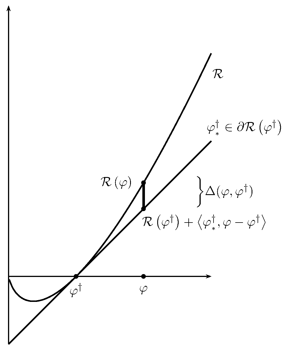
Figure 1: Bregman distance

$$\Delta(\varphi,\varphi^{\dagger})=\|\varphi-\varphi^{\dagger}\|_{\mathcal{X}}^{2}.$$

Although, Bregman distances are in general not metrics they have meaningful interpretations in some Banach space settings. If $\mathcal{X}=L^{1}(D)$ and $\mathcal{R}(\varphi)=\int_{D}\varphi(x)\ln(\varphi(x))\,dx$ (entropy regularization), then $\Delta(\varphi,\varphi^{\dagger})$ can be bounded from below by $\|\varphi-\varphi^{\dagger}\|_{L^{1}}^{2}$ (see e.g.Resmerita (2005)), i.e. the error bounds formulated in the next theorem can be interpreted as bounds with respect to the squared $L^{1}$ norm. Our framework also allows the incorporation of convex constraints by setting $\mathcal{R}(\varphi):=\infty$ if $\varphi$ does not belong to some convex set $\mathcal{C}$. Obviously, this does not change $\Delta$ in $\mathcal{C}$.

Following Kaltenbacher and Hofmann (2010) we formulate the source condition as a variational inequality

$$\left\langle\varphi^{\dagger}_{*},\varphi^{\dagger}-\varphi\right\rangle\leq\beta\Delta(\varphi,\varphi^{\dagger})^{1/2}\Lambda\left(\frac{\|\mathcal{F}^{\prime}[\varphi^{\dagger}](\varphi-\varphi^{\dagger})\|^{2}}{\Delta(\varphi,\varphi^{\dagger})}\right)\qquad\mbox{for all }\varphi\in\mathfrak{B}.$$ (22)

Again, this is a generalization of the Hilbert space case. It is shown in Kaltenbacher and Hofmann (2010) that if $\mathcal{X}$ is a Hilbert space, $\mathcal{R}(\varphi)=\|\varphi-\varphi_{0}\|^{2}$ and $(\Lambda^{2})^{-1}$ is convex, the classical source condition (20) implies the variational one (22).

Let us close this section with a technical remark. Note that if $\mathfrak{B}$ is chosen such that $\varphi^{\dagger}$ is on the boundary of $\mathfrak{B}$, then possibly $\Lambda$ can be chosen smaller than in the case where $\varphi^{\dagger}$ is in the interior of $\mathfrak{B}$. Theorem 1 yields that this may lead to faster rates of convergence. Hence, a convex constraint on the regression function can improve estimation. To captures this fact it is important that, opposed to the formulation in Kaltenbacher and Hofmann (2010), no absolute values appear on the left hand side of (22). A typical example where $\varphi^{\dagger}$ is on the boundary of $\mathfrak{B}$ is the assumption that $\varphi^{\dagger}$ is a positive function.

4 Convergence results

Let $\mathcal{X}$ be a Banach space, $\mathcal{Y}$ a Hilbert space, $\mathfrak{B}\subset\mathcal{X}$ convex and $\varphi^{\dagger}\in\mathfrak{B}$ a root of the operator $\mathcal{F}:\mathfrak{B}\to\mathcal{Y}$:

$$\mathcal{F}(\varphi^{\dagger})=0.$$ (23)

Assume that $\mathcal{F}$ is approximated by a series of estimators

$$\widehat{\mathcal{F}}_{n}:\mathfrak{B}\to\widehat{\mathcal{Y}}_{n}$$

which maps to some (possibly finite-dimensional and/or data dependent) Hilbert space $\widehat{\mathcal{Y}}_{n}$. $\mathcal{F}$ and all $\widehat{\mathcal{F}}_{n}$ are assumed to be Gateaux differentiable on $\mathfrak{B}$ with linear derivatives $\mathcal{F}^{\prime}[\varphi]$ and $\widehat{\mathcal{F}}_{n}^{\prime}[\varphi]$, which are “bounded with respect to $\Delta$” in the sense that

$$\sup_{\{\tilde{\varphi}\in\mathfrak{B}:\Delta(\tilde{\varphi},\varphi)\neq 0\}}\|\mathcal{F}^{\prime}[\varphi](\tilde{\varphi}-\varphi)\|^{2}/\Delta(\tilde{\varphi},\varphi)<\infty\quad\text{and}\quad\mathcal{F}^{\prime}[\varphi](\tilde{\varphi}-\varphi)\neq 0$$ (24)

whenever $\Delta(\tilde{\varphi},\varphi)\neq 0$ and analogously for all $\widehat{\mathcal{F}}_{n}$. Now we can state the main theorem of this paper, which is proved in Appendix A:

Theorem 1.

Let (22) hold true with a concave $\Lambda$ for which $t\mapsto\sqrt{t}/\Lambda(t)$ is monotonically increasing. Assume that the sequence $\widehat{\mathcal{F}}_{n}$ has the following convergence properties:

$$\|\widehat{\mathcal{F}}_{n}(\varphi^{\dagger})\|=O_{p}(\delta_{n}),$$ (25a)

$$\left(\left|\sup_{\varphi\in\mathfrak{B}}\frac{\|\mathcal{F}^{\prime}[\varphi^{\dagger}](\varphi-\varphi^{\dagger})\|^{2}-\|\widehat{\mathcal{F}}_{n}^{\prime}[\varphi^{\dagger}](\varphi-\varphi^{\dagger})\|^{2}}{\Delta(\varphi,\varphi^{\dagger})}\right|\right)^{1/2}=O_{p}(\gamma_{n}),$$ (25b)

$$\begin{split}&P\{\|\widehat{\mathcal{F}}_{n}(\varphi_{1})-\widehat{\mathcal{F}}_{n}(\varphi_{2})-\widehat{\mathcal{F}}_{n}^{\prime}[\varphi_{2}](\varphi_{1}-\varphi_{2})\|>\eta\|\widehat{\mathcal{F}}_{n}(\varphi_{1})-\widehat{\mathcal{F}}_{n}(\varphi_{2})\|\\ &\hskip 221.93149pt\text{ for some }\varphi_{1},\varphi_{2}\in\mathfrak{B}\}\rightarrow 0.\end{split}$$ (25c)

Here $\eta$ must be sufficiently small, such that $4\eta(1+\eta)(1-\eta)^{-3}<q^{-3/2}$. Suppose that the convex minimization problems (3) are uniquely solvable for every $\widehat{\mathcal{F}}_{n}$ (see Remark 1 for sufficient conditions), i.e. the method is well defined. Further assume that $\alpha_{0}>\max(\Theta^{-1}(\delta_{n}),\gamma_{n}^{2})$ and that $\alpha_{k}\leq q\alpha_{k+1}$ for all $k$ with a constant $q>1$. Let the iteration be stopped at the smallest index $K_{n}\in\mathbb{N}_{0}$ for which

$$\alpha_{K_{n}+1}\leq\max(\Theta^{-1}(\delta_{n}),\gamma_{n}^{2})\,,\qquad\mbox{where }\Theta(t):=\sqrt{t}\Lambda(t).$$ (26)

Then

$$\Delta(\widehat{\varphi}_{K_{n}},\varphi^{\dagger})=O_{p}\left(\Lambda^{2}\left(\max(\Theta^{-1}(\delta_{n}),\gamma_{n}^{2})\right)\right)$$

Remarks:

1. Sufficient conditions for uniqueness of solutions to the minimization problem (3) are strict convexity of $\mathcal{R}$ or injectivity of $\widehat{\mathcal{F}}_{n}^{\prime}[\widehat{\varphi}_{k-1}]$.

2. Sufficient conditions for existence are reflexivity of $\mathcal{X}$, weak closedness of $\mathfrak{B}$, and the boundedness of the sets $\{\varphi\in\mathfrak{B}:\mathcal{R}(\varphi)\leq R\}$ in $\mathcal{X}$ for any $R\in\mathbb{R}$. This is a standard argument: If $(\varphi_{n})$ is a minimizing sequence, it must be bounded due to our last condition. Since $\mathcal{X}$ is reflexive, there exists a weakly convergent subsequence, and by weak closedness of $\mathfrak{B}$ a weak limit point $\varphi_{*}\in\mathfrak{B}$. Since the Tikhonov functional is convex and lower semi-continuous, it is also weakly lower semi-continuous, and hence $\varphi_{*}$ is a minimizer.

3. Note that if $\mathcal{X}$ is a Hilbert space and $\widehat{\mathcal{F}}_{n}$ Fréchet differentiable, then $\|\mathcal{F}^{\prime}[\varphi^{\dagger}](\varphi-\varphi^{\dagger})\|^{2}-\|\widehat{\mathcal{F}}_{n}^{\prime}[\varphi^{\dagger}](\varphi-\varphi^{\dagger})\|^{2}\leq\|\mathcal{F}^{\prime}[\varphi^{\dagger}]^{*}\mathcal{F}^{\prime}[\varphi^{\dagger}]-\widehat{\mathcal{F}}_{n}^{\prime}[\varphi^{\dagger}]^{*}\widehat{\mathcal{F}}_{n}^{\prime}[\varphi^{\dagger}]\|\;\|\varphi-\varphi^{\dagger}\|^{2}$, so $\gamma_{n}\leq\|\mathcal{F}^{\prime}[\varphi^{\dagger}]^{*}\mathcal{F}^{\prime}[\varphi^{\dagger}]-\widehat{\mathcal{F}}_{n}^{\prime}[\varphi^{\dagger}]^{*}\widehat{\mathcal{F}}_{n}^{\prime}[\varphi^{\dagger}]\|^{1/2}$.

4. The bound on the Taylor remainder of $\widehat{\mathcal{F}}_{n}$

   $$\|\widehat{\mathcal{F}}_{n}(x)-\widehat{\mathcal{F}}_{n}(y)-\widehat{\mathcal{F}}_{n}^{\prime}[y](x-y)\|\leq\eta\|\widehat{\mathcal{F}}_{n}(x)-\widehat{\mathcal{F}}_{n}(y)\|,$$ (27)

   used in (LABEL:eq:probtc) is known as the tangential cone condition. This condition is commonly used in the analysis of regularization methods for nonlinear ill-posed problems, see Kaltenbacher et al. (2008). The right hand side of (27) may be replaced by $\|F^{\prime}[y](x-y)\|$ (see (39) below), and in this form it corresponds to Assumption 2 in Chen et al. (2011).

Corollary 2.

Let the assumptions of Theorem 1 hold true.

1. If $\Lambda(t)=t^{\mu}$ for some $\mu\in(0,1/2]$ (Hölder-type source conditions), then

   $$\Delta(\widehat{\varphi}_{K},\varphi^{\dagger})^{1/2}=O_{p}\left(\max(\delta_{n}^{2\mu/(2\mu+1)},\gamma_{n}^{2\mu})\right)\,.$$ (28)

2. If $\mathcal{F}$ is scaled such that $\|\mathcal{F}^{\prime}[\varphi^{\dagger}](\varphi-\varphi^{\dagger})\|^{2}/\Delta(\varphi,\varphi^{\dagger})\leq\frac{1}{2}$ and $\Lambda(t)=(-\ln t)^{-p}$ for some $p>0$ (logarithmic source conditions), then

   $$\Delta(\widehat{\varphi}_{K},\varphi^{\dagger})^{1/2}=O_{p}\left((-\ln\max(\delta_{n},\gamma_{n}))^{-p}\right)$$ (29)

   for all $\delta_{n},\gamma_{n}$ sufficiently small.

Let us discuss some properties of the method. First of all it is a local method like any Newton method. Convergence is only guaranteed if the initial guess $\varphi_{0}$ is sufficiently close to the true solution $\varphi^{\dagger}$. How close it has to be depends on the special problem, i.e. the operator $\mathcal{F}$. This property appears in the assumptions (22) and (LABEL:eq:probtc) in Theorem 1.

We emphasized in the introduction that the method requires only solutions of convex minimization problems. Therefore, it does not suffer from the problem of multiple local minima which frequently occur in nonlinear Tikhonov regularization (2) and make it hard to find the actual minimum.

Unlike for nonlinear Tikhonov regularization our theoretical results do not require the strong assumption that we can always find the minimum of a functional with an arbitrary number of local minima. In turn we have to assume (LABEL:eq:probtc), which is usually hard to check. Although, rigorous proofs for (LABEL:eq:probtc) are often missing, it seems to hold in many cases at least in a neighborhood of $\varphi^{\dagger}$.

An important advantage for the numerical implementation is that a lot of efficient algorithms converging always towards the true solution are known for convex minimization problems. The error of these minimization algorithms plays a minor role compared to the regularization error for the applications of Section 2. We refer to Langer and Hohage (2007) for a detailed discussion of the interplay of these errors in other applications.

5 Examples revisited

The assumptions of Theorem 1 and Corollary 2 are rather abstract and need some explanations concerning the application to the nonparametric regression with independent instrument (4). They are applicable in a similar way to the nonparametric quantile regression (7). In (10) the operator $\mathcal{F}$ for the regression with independent instrument is an integral operator with a kernel composed by marginals of $f_{YZW}$. Hence, an estimator $\widehat{f}_{YZW}$ yields an estimator of the kernel and thereby of $\widehat{\mathcal{F}}$.

Condition (24) that all $\widehat{\mathcal{F}}_{n}^{\prime}[\varphi]$ must be bounded with respect to the Bregman distance is fulfilled if the derivatives of $\mathcal{F}$ are bounded according to (24), the estimation of $f_{YZW}$ is strongly consistent and $n$ is large enough. Strong consistency is established for many density estimators. The boundedness of $\mathcal{F}$ with respect to the Bregman distance is reasonable. It holds if the partial derivative of the joint density $\frac{\partial}{\partial y}f_{YZW}$ is bounded for the operator (10) or if $f_{YZ|W}$ is bounded for the operator (12) and the Bregman distance is bounded from below by the power of a norm. As mentioned in Section 3.3, the latter is for example the case for quadratic and maximum entropy penalty.

It can be argued with strong consistency as well that the probabilistic tangential cone condition (LABEL:eq:probtc) holds if the exact operator $\mathcal{F}$ fulfills the tangential cone condition (27). But, it is known that a verification, whether or not the tangential cone condition is true, is often difficult for a given operator.

In analogy to (12) the operator

$$\tilde{\mathcal{F}}(\varphi)(u,w):=\left(\begin{array}[]{c}\mathbb{P}\big{(}Y-\varphi(Z)\leq u\big{)}-\mathbb{P}\big{(}Y-\varphi(Z)\leq u|W=w\big{)}\\ \mathbb{E}[\varphi(Z)-Y]\end{array}\right)$$

can be considered for model (4). With this operator the conditions (24) and (27) are more explicitly assumptions on the primitives of the model.

In the rates for Hölder source conditions (28) in Corollary 2, $\delta$ has a smaller exponent than $\gamma$. However $\delta$ does not necessarily dominate the convergence. In the nonparametric instrumental regression $\delta$ corresponds to the estimation of a density, while $\gamma$ is determined by the estimation of a partial derivative of that density. Hence, $\gamma$ decays usually slower than $\delta$. Which of the terms $\delta^{2\mu/(2\mu+1)}$ or $\gamma^{2\mu}$ dominates the convergence depends on the properties of the special problem, namely the number of instruments and covariates as well as on the smoothness of the density and the initial error $\varphi^{\dagger}-\varphi_{0}$.

The situation becomes clearer in the case of logarithmic source conditions. If the kernel of the operator is analytic, but the initial error in the regression function is not smooth or has only finite Hölder smoothness, merely a logarithmic rate of convergence can be expected. As discussed in Section 3.2 this situation can occur in many applications. Even for estimating an analytic density a nonparametric density estimator will attain only a polynomial rate in $n$. Due to (29) our estimator for $\varphi$ will end up asymptotically with the logarithmic rate $(-\ln(n))^{-p}$.

6 Numerical simulations

In this section we present some numerical simulations for nonparametric instrumental regression with independent binary instrument and real-valued continuous explanatory and dependent variables. This leads to the nonlinear operator equation (18). Our simulations show that the solution computed by the method (3) approximates the exact solution. As mentioned above, due to dimensionality, the regression function cannot be identified with a binary instrument if the standard regression model (5) is used.

In our simulations we choose $Y$ as real valued, $Z$ with values in $[0,1]$ and $W$ with values in $\{0,1\}$. We assume the regression function is

$$\varphi^{\dagger}(z)=\frac{1}{6}\sin(2\pi(z+0.25))+0.41\,,\qquad z\in[0,1]\,.$$

Moreover, we take $w_{0}=P(W=0)=2/3$ and $w_{1}=P(W=1)=1/3$. To make $Z$ endogenous, let us choose the error term as $(U|Z=z,W=w)\sim\mathcal{N}(\mu_{w}(z),0.09^{2})$ with $\mu_{0}(z):=0.2z-0.1$ and $\mu_{1}(z):=0.25z-0.125$. The functions $\mu_{0}(z)$ and $\mu_{1}(z)$ describe precisely the correlation between the explanatory variable and the error term, which should be removed using the information contained in the instrumental variable. Although $U$ varies with $Z$ and $W$ the condition $W\mathchoice{\mathrel{\hbox to0.0pt{$\displaystyle\perp$\hss}\mkern 2.0mu{\displaystyle\perp}}}{\mathrel{\hbox to0.0pt{$\textstyle\perp$\hss}\mkern 2.0mu{\textstyle\perp}}}{\mathrel{\hbox to0.0pt{$\scriptstyle\perp$\hss}\mkern 2.0mu{\scriptstyle\perp}}}{\mathrel{\hbox to0.0pt{$\scriptscriptstyle\perp$\hss}\mkern 2.0mu{\scriptscriptstyle\perp}}}U$ can be assured by a proper choice of $f_{Z,W}(z,w)$. We write the joint density as

$$\begin{split}f_{YZW}(y,z,0)=f_{ZW}(z,0)\frac{1}{0.09\sqrt{2\pi}}\exp\left(-\frac{1}{2}\left(\frac{y-\varphi^{{\dagger}}(z)-\mu_{0}(z)}{0.09}\right)^{2}\right),\\ f_{YZW}(y,z,1)=f_{ZW}(z,1)\frac{1}{0.09\sqrt{2\pi}}\exp\left(-\frac{1}{2}\left(\frac{y-\varphi^{{\dagger}}(z)-\mu_{1}(z)}{0.09}\right)^{2}\right).\end{split}$$ (30)

Now $f_{ZW}$ has to be determined such that $W$ and $U$ are independent, which is equivalent to (17). Let us show that setting $f_{ZW}(z,1):=0.625f_{ZW}(1.25z-0.125,0)$ achieves this. With a substitution of variables we compute

$$\begin{split}&\int w_{1}f_{YZW}(u+\varphi^{{\dagger}}(z),z,0)\,dz\\ =&\int\frac{1}{3}f_{ZW}(z,0)\frac{1}{0.09\sqrt{2\pi}}\exp\left(-\frac{1}{2}\left(\frac{u-0.2z+0.1)}{0.09}\right)^{2}\right)\,dz\\ =&\int\frac{1.25}{3}f_{ZW}(1.25v-0.125,0)\frac{1}{0.09\sqrt{2\pi}}\exp\left(-\frac{1}{2}\left(\frac{u-0.25v+0.125)}{0.09}\right)^{2}\right)\,dv\\ =&\int w_{0}f_{YZW}(u+\varphi^{{\dagger}}(v),v,1)\,dv.\end{split}$$

This shows that (17) holds with our definition of $f_{ZW}(z,1)$ what ever $f_{ZW}(z,0)$ looks like. Here we take it to be normally distributed with variance $0.3^{2}$ and expectation $1/2$ truncated to the interval $[0,1]$, i.e.

$$f_{ZW}(z,0):=a\exp\left(-\frac{1}{2}\left(\frac{z-1/2}{0.3}\right)^{2}\right),\qquad z\in[0,1]$$

with some scaling factor $a$ chosen such that $\int_{0}^{1}f_{ZW}(z,0)dz=2/3$. By this construction, the error term also meets the condition $\mathbb{E}U=0$ of the regression model (4): To see this, note that $f_{ZW}(\cdot,0)$ and $f_{ZW}(\cdot,1)$ are even, while $\mu_{0}$ and $\mu_{1}$ are odd functions with respect to the point $0.5$. Hence,

$$\begin{split}\mathbb{E}U&=\int w_{0}f_{Z,W}(z,0)\mathbb{E}(U|Z=z,W=0)+w_{1}f_{Z,W}(z,1)\mathbb{E}(U|Z=z,W=1)\,dz\\ &=\int w_{0}f_{Z,W}(z,0)\mu_{0}(z)+w_{1}f_{Z,W}(z,1)\mu_{1}(z)\,dz=0.\end{split}$$

This construction allows an easy formulation of how the solution of a nonparametric regression without instrumental variable and without noise would look like: $\widetilde{\varphi}(z)=w_{0}\mu_{0}(z)+w_{1}\mu_{1}(z)+\varphi^{\dagger}$

Figure 2: Necessity of the instrument: A standard regression would asymptotically yield a curve which is far away from the true solution $\varphi^{\dagger}$.

To approximately solve the integral operator equation (18) by the method (3) we discretized the domain $[0,1]\times[0,1]\times\{0,1\}$ by $256\times 256\times 2$ points and chose the regularization parameters by $\alpha_{0}=1$ and $\alpha_{n+1}=0.9\alpha_{n}$. The iteration was stopped using Lepskiĭ’s principle as in Bauer, Hohage & Munk Bauer et al. (2009). The initial guess was chosen as the constant function $E[Y]$. For a first test we used the exact density $f_{YZW}$, which actually has to be estimated from the data, of course. The $L^{2}$-error was reduced from $0.1294$ to $0.0028$. The remaining error is due to discretization noise. This suggests that the example is identifiable and can be solved by the method (3). Compared to the error for densities estimated from simulated data below, the observed discretization error is very small. Hence, the discretization is fine enough and discretization error is insignificant for our simulations. The singular values of $\mathcal{F}^{\prime}[\varphi^{\dagger}]$ are shown in Figure 4. They exhibit an exponential decay, so according to Corollary 2 we can only expect slow rates of convergence.
Figure 3: Result of the iterative inversion using the exact density $f_{YZW}$.   Figure 4: Singular values of $\mathcal{F}^{\prime}[\varphi^{\dagger}]$
In further tests the algorithm was evaluated for finite samples of $(Y,Z,W)$ with $10^{3}$, $10^{4}$ and $10^{5}$ points. Given such a sample, the joint density $f_{YZW}$ was estimated non-parametrically by the kernel density estimator developed by Botev, Grotowski & Kroese Botev et al. (2010). Afterwards again (18) was solved, but the exact density was replaced by the estimated one. We made $1000$ samples for each tested sample size. The following table and histograms in Fig. 5–7 show the $L^{2}$-errors of the approximate solution normed by the error of the initial guess (i.e. the error of the initial guess is $1$). It can be seen that small samples produce unwanted outliers, but the method becomes reliable when the sample size is large enough. Fig. 8–10 show median reconstructions for each sample size. The results demonstrate that our method computes an asymptotically correct estimator of the regression function $\varphi^{{\dagger}}$ with an endogeneous explanatory variable $Z$ using only a binary instrument $W$.

the exact solution is $0$ and the error of the initial guess is $1$. It can be seen that small samples produce unwanted outliers, but that the method becomes reliable, when the sample is large enough.

sample size $N$	mean	quantiles	$p=0.25$	$p=0.5$	$p=0.75$	$p=0.9$
$10^{3}$	0.6159		0.4057	0.5751	0.7921	0.9575
$10^{4}$	0.3694		0.2496	0.3524	0.4574	0.5729
$10^{5}$	0.3264		0.2592	0.3278	0.3882	0.4610

Figure 5: $L^{2}$ error for sample size $N=10^{3}$

Figure 6: $L^{2}$ error for sample size $N=10^{4}$

Figure 7: $L^{2}$ error for sample size $N=10^{5}$

Figure 8: Median reconstruction, $N=10^{3}$

Figure 9: Median reconstruction, $N=10^{4}$

Figure 10: Median reconstruction, $N=10^{5}$

Appendix A Proof of the main theorem

Before we come to the proof of Theorem 1, let us first formulate a result with deterministic error in the operator. We assume that $\mathcal{F}$ is approximated by some deterministic operator

$$\widehat{\mathcal{F}}:\mathfrak{B}\to\widehat{\mathcal{Y}}.$$

Let both $\mathcal{F}$ and $\widehat{\mathcal{F}}$ be Gateaux differentiable on $\mathfrak{B}$ with derivatives $\mathcal{F}^{\prime}[\varphi]$ and $\widehat{\mathcal{F}}^{\prime}[\varphi]$, which are “bounded with respect to $\Delta$” in the sense that $\sup_{\{\tilde{\varphi}\in\mathfrak{B}:\Delta(\tilde{\varphi},\varphi)\neq 0\}}\|\mathcal{F}^{\prime}[\varphi](\tilde{\varphi}-\varphi)\|^{2}/\Delta(\tilde{\varphi},\varphi)<\infty$ and $\mathcal{F}^{\prime}[\varphi](\tilde{\varphi}-\varphi)\neq 0$ whenever $\Delta(\tilde{\varphi},\varphi)\neq 0$ and analogously for $\widehat{\mathcal{F}}$. The error of the approximation is described by:

$$\delta := \|\widehat{\mathcal{F}}(\varphi^{\dagger})\|,$$ (31a)

$$\gamma := \left(\left|\sup_{\{\varphi\in\mathfrak{B}:\Delta(\varphi,\varphi^{\dagger})\neq 0\}}\frac{\|\mathcal{F}^{\prime}[\varphi^{\dagger}](\varphi-\varphi^{\dagger})\|^{2}-\|\widehat{\mathcal{F}}^{\prime}[\varphi^{\dagger}](\varphi-\varphi^{\dagger})\|^{2}}{\Delta(\varphi,\varphi^{\dagger})}\right|\right)^{1/2}.$$ (31b)

Moreover, we assume that the tangential cone condition

$$\|\widehat{\mathcal{F}}(x)-\widehat{\mathcal{F}}(y)-\widehat{\mathcal{F}}^{\prime}[y](x-y)\|\leq\eta\|\widehat{\mathcal{F}}(x)-\widehat{\mathcal{F}}(y)\|,$$ (32)

holds for all $x,y$ in some neighborhood of $\mathcal{B}$.

Lemma 3.

Assume that (22), (31) and (32) hold true with $\eta$ sufficiently small, such that

$$4\eta(1+\eta)(1-\eta)^{-3}<q^{-3/2}.$$ (33)

Further assume that the convex minimization problems (3) are uniquely solvable and that the iteration is stopped at the smallest index $K\in\mathbb{N}_{0}$ for which

$$\alpha_{K+1}\leq\max(\Theta^{-1}(\delta),\gamma^{2})\,,\qquad\mbox{where }\Theta(t):=\sqrt{t}\Lambda(t).$$ (34)

In addition it should hold that $\alpha_{0}>\max(\Theta^{-1}(\delta),\gamma^{2})$ and $\alpha_{k}\leq q\alpha_{k+1}$ for all $k$ with a constant $q>1$. Moreover, let $\Lambda$ be concave and assume that $t\mapsto\sqrt{t}/\Lambda(t)$ is monotonically increasing.

Then there exists a constant $C>0$ independent of the $\widehat{\mathcal{F}}$ such that

$$\Delta(\widehat{\varphi}_{K},\varphi^{\dagger}) \leq C\left(\Lambda\left(\max(\Theta^{-1}(\delta),\gamma^{2})\right)\right)^{2}\,.$$ (35)

Proof.

Let us introduce the following notation:

$$\mathcal{T}:=\mathcal{F}^{\prime}[\varphi^{\dagger}],\qquad\widehat{\mathcal{T}}:=\widehat{\mathcal{F}}^{\prime}[\varphi^{\dagger}],\qquad\widehat{\mathcal{T}}_{k-1}:=\widehat{\mathcal{F}}^{\prime}[\widehat{\varphi}_{k-1}],$$

$$\Delta_{k}:=\Delta(\widehat{\varphi}_{k},\varphi^{\dagger}),\qquad e_{k}:=\widehat{\varphi}_{k}-\varphi^{\dagger}.$$

From the optimality condition (3) with $\varphi=\varphi^{\dagger}$ we find that

$$\begin{split}&\|\widehat{\mathcal{T}}_{k-1}(\widehat{\varphi}_{k}-\widehat{\varphi}_{k-1})+\widehat{\mathcal{F}}(\widehat{\varphi}_{k-1})\|^{2}+\alpha_{k}\mathcal{R}(\widehat{\varphi}_{k})\\ &\qquad\leq\|\widehat{\mathcal{T}}_{k-1}(\varphi^{\dagger}-\widehat{\varphi}_{k-1})+\widehat{\mathcal{F}}(\widehat{\varphi}_{k-1})\|^{2}+\alpha_{k}\mathcal{R}(\varphi^{\dagger}).\end{split}$$ (36)

From the definition (21) of the Bregman distance and the source condition (22) we obtain

$$\mathcal{R}(\varphi^{\dagger})-\mathcal{R}(\widehat{\varphi}_{k})=\left\langle\varphi^{\dagger}_{*},\varphi^{\dagger}-\widehat{\varphi}_{k}\right\rangle-\Delta_{k}\;\leq\;\beta\Delta_{k}^{1/2}\Lambda\left(\frac{\|\mathcal{T}e_{k}\|^{2}}{\Delta_{k}}\right)-\Delta_{k}.$$ (37)

Plugging this into (36) yields

$$\begin{split}&\|\widehat{\mathcal{T}}_{k-1}(\widehat{\varphi}_{k}-\widehat{\varphi}_{k-1})+\widehat{\mathcal{F}}(\widehat{\varphi}_{k-1})\|^{2}+\alpha_{k}\Delta_{k}\\ &\qquad\leq\|\widehat{\mathcal{T}}_{k-1}(\varphi^{\dagger}-\widehat{\varphi}_{k-1})+\widehat{\mathcal{F}}(\widehat{\varphi}_{k-1})\|^{2}+\beta\alpha_{k}\Delta_{k}^{1/2}\Lambda\left(\frac{\|\mathcal{T}e_{k}\|^{2}}{\Delta_{k}}\right)\,.\end{split}$$ (38)

Note that the tangential cone condition (32) implies

$$(1+\eta)^{-1}\|\widehat{\mathcal{T}}e_{k}\|\leq\|\widehat{\mathcal{F}}(\widehat{\varphi}_{k})-\widehat{\mathcal{F}}(\varphi^{\dagger})\|\leq(1-\eta)^{-1}\|\widehat{\mathcal{T}}e_{k}\|\,.$$ (39)

To estimate the first term on the left hand side of (38) we use (32) and (39) to get that

$$\|\widehat{\mathcal{F}}(\widehat{\varphi}_{k})\|-\|\widehat{\mathcal{T}}_{k-1}(\widehat{\varphi}_{k}-\widehat{\varphi}_{k-1})+\widehat{\mathcal{F}}(\widehat{\varphi}_{k-1})\|$$

$$\leq \|\widehat{\mathcal{T}}_{k-1}(\widehat{\varphi}_{k}-\widehat{\varphi}_{k-1})+\widehat{\mathcal{F}}(\widehat{\varphi}_{k-1})-\widehat{\mathcal{F}}(\widehat{\varphi}_{k})\|$$

$$\leq \eta\|\widehat{\mathcal{F}}(\widehat{\varphi}_{k-1})-\widehat{\mathcal{F}}(\widehat{\varphi}_{k})\|$$

$$\leq \eta\|\widehat{\mathcal{F}}(\widehat{\varphi}_{k-1})-\widehat{\mathcal{F}}(\varphi^{\dagger})\|+\eta\|\widehat{\mathcal{F}}(\widehat{\varphi}_{k})-\widehat{\mathcal{F}}(\varphi^{\dagger})\|$$

$$\leq \frac{\eta}{1-\eta}(\|\widehat{\mathcal{T}}e_{k}\|+\|\widehat{\mathcal{T}}e_{k-1}\|).$$

Together with $\||\widehat{\mathcal{F}}(\widehat{\varphi}_{k})\|\geq\|\widehat{\mathcal{F}}(\widehat{\varphi}_{k})-\widehat{\mathcal{F}}(\varphi^{\dagger})\|-\delta\geq(1+\eta)^{-1}\|\widehat{\mathcal{T}}e_{k}\|-\delta$ this yields

$$\|\widehat{\mathcal{T}}_{k-1}(\widehat{\varphi}_{k}-\widehat{\varphi}_{k-1})+\widehat{\mathcal{F}}(\widehat{\varphi}_{k-1})\|\geq\frac{(1-\eta)^{2}}{1-\eta^{2}}\|\widehat{\mathcal{T}}e_{k}\|-\frac{\eta}{1-\eta}\|\widehat{\mathcal{T}}e_{k-1}\|-\delta.$$

For the right hand side of (38) we get from (31) and another application of (32) that

$$\|\widehat{\mathcal{T}}_{k-1}(\varphi^{\dagger}-\widehat{\varphi}_{k-1})+\widehat{\mathcal{F}}(\widehat{\varphi}_{k-1})\|\leq\eta\|\widehat{\mathcal{F}}(\widehat{\varphi}_{k-1})-\widehat{\mathcal{F}}(\varphi^{\dagger})\|+\delta\leq\frac{\eta}{1-\eta}\|\widehat{\mathcal{T}}e_{k-1}\|+\delta.$$

Plugging the last two inequalities into (38) and using the simple inequalities $(a-b)^{2}\geq\frac{1}{2}a^{2}-b^{2}$ and $(a+b)^{2}\leq 2a^{2}+2b^{2}$ we obtain that

$$\begin{split}&\underbrace{\frac{1}{2}\left(\frac{(1-\eta)^{2}}{1-\eta^{2}}\right)^{2}}_{=:C_{\eta}}\left\|\widehat{\mathcal{T}}e_{k}\right\|^{2}+\alpha_{k}\Delta_{k}\leq\underbrace{\frac{4\eta^{2}}{(1-\eta)^{2}}}_{=:c_{\eta}}\left\|\widehat{\mathcal{T}}e_{k-1}\right\|^{2}+4\delta^{2}+\beta\alpha_{k}\Delta_{k}^{1/2}\Lambda\left(\frac{\|\mathcal{T}e_{k}\|^{2}}{\Delta_{k}}\right)\,.\end{split}$$

Using (31b) and the monotonicity of $\Lambda$ we find that $\Lambda\left(\frac{\|\mathcal{T}e_{k}\|^{2}}{\Delta_{k}}\right)\leq\Lambda\left(\frac{\|\widehat{\mathcal{T}}e_{k}\|^{2}}{\Delta_{k}}+\gamma^{2}\right)$. Together with the stopping rule (34) this implies

$$C_{\eta}\|\widehat{\mathcal{T}}e_{k}\|^{2}+\alpha_{k}\Delta_{k}\leq c_{\eta}\|\widehat{\mathcal{T}}e_{k-1}\|^{2}+4\Theta(\alpha_{k})^{2}+\beta\alpha_{k}\Delta_{k}^{1/2}\Lambda\left(\frac{\|\widehat{\mathcal{T}}e_{k}\|^{2}}{\Delta_{k}}+\alpha_{k}\right)\,.$$ (40)

We will show the following error bounds

$$\|\widehat{\mathcal{T}}e_{k}\|^{2} \leq C_{1}\Theta(\alpha_{k})^{2},$$ (41a)

$$\Delta(\widehat{\varphi}_{k},\varphi^{\dagger}) \leq C_{2}\Lambda(\alpha_{k})^{2}$$ (41b)

with

$$C_{1} := \max\left(\dfrac{\|\widehat{\mathcal{T}}e_{0}\|^{2}}{\Theta(\alpha_{0})^{2}},\,\dfrac{8}{C_{\eta}-2q^{3}c_{\eta}},\,\dfrac{16\beta^{2}}{C_{\eta}+1},\,\dfrac{16\beta^{2}}{C_{\eta}^{2}}\right),$$

$$C_{2} := \max\left(\dfrac{\Delta(\varphi_{0},\varphi^{\dagger})}{\Lambda(\alpha_{0})^{2}},\,2C_{1}c_{\eta}q^{3}+8,\,16\beta^{2},\,\frac{16\beta^{2}}{C_{\eta}}\right).$$

We will prove these claims by induction in $k\leq K$. For $k=0$ this is arranged by the definitions of $C_{1}$ and $C_{2}$. For the induction step we distinguish two cases:

Case 1: $c_{\eta}\|\widehat{\mathcal{T}}e_{k-1}\|^{2}+4\Theta(\alpha_{k})^{2}\geq\beta\alpha_{k}\Delta_{k}^{1/2}\Lambda\left(\frac{\|\widehat{\mathcal{T}}e_{k}\|^{2}}{\Delta_{k}}+\alpha_{k}\right)$.
Now by using the induction hypothesis (41a) equation (40) simplifies to

$$C_{\eta}\|\widehat{\mathcal{T}}e_{k}\|^{2}+\alpha_{k}\Delta_{k}\leq 2c_{\eta}C_{1}\Theta(\alpha_{k-1})^{2}+8\Theta(\alpha_{k})^{2}.$$

We have $\Theta(\alpha_{k-1})=(\alpha_{k-1})^{1/2}\Lambda(\alpha_{k-1})\leq(q\alpha_{k})^{1/2}\Lambda(q\alpha_{k})$ as $\Lambda$ is monotonically increasing. While $\Lambda$ is concave and $\Lambda(0)=0$ the definition of concavity implies $t\Lambda(x)\leq\Lambda(tx)$ for $0\geq t\geq 1$. Now taking $x=q\alpha_{k}$ and $t=q^{-1}$ gives $\Lambda(q\alpha_{k})\leq q\Lambda(\alpha_{k})$ and therefore

$$\Theta(\alpha_{k-1})\leq q^{3/2}\Theta(\alpha_{k}).$$

Putting the last two equations together results into the bound

$$C_{\eta}\|\widehat{\mathcal{T}}e_{k}\|^{2}+\alpha_{k}\Delta_{k}\leq(2c_{\eta}C_{1}q^{3}+8)\Theta(\alpha_{k})^{2}=(2c_{\eta}C_{1}q^{3}+8)\alpha_{k}\Lambda(\alpha_{k})^{2}.$$

Firstly, this implies by omitting the second term on the left hand side that

$$\|\widehat{\mathcal{T}}e_{k}\|^{2}\leq\dfrac{2c_{\eta}C_{1}q^{3}+8}{C_{\eta}}\Theta(\alpha_{k})^{2}\quad\text{and hence}\quad C_{1}\geq\dfrac{2c_{\eta}C_{1}q^{3}+8}{C_{\eta}}.$$

Hence, it is necessary that $C_{\eta}>2q^{3}c_{\eta}$, which is equivalent to the inequality (33) assumed in the Lemma. Then (41a) is true with $C_{1}\geq\dfrac{8}{C_{\eta}-2q^{3}c_{\eta}}$.

Secondly, omitting the first term of the left hand side shows $\Delta_{k}\leq(2c_{\eta}C_{1}q^{3}+8)\Lambda(\alpha_{k})^{2}$, so we have (41b) with $C_{2}\geq 2c_{\eta}C_{1}q^{3}+8$.

Case 2: $\beta\alpha_{k}\Delta_{k}^{1/2}\Lambda\left(\frac{\|\widehat{\mathcal{T}}e_{k}\|^{2}}{\Delta_{k}}+\alpha_{k}\right)\geq c_{\eta}\|\widehat{\mathcal{T}}e_{k-1}\|^{2}+4\Theta(\alpha_{k})^{2}$.
In this case (40) simplifies to

$$C_{\eta}\|\widehat{\mathcal{T}}e_{k}\|^{2}+\alpha_{k}\Delta_{k}\leq 2\beta\alpha_{k}\Delta_{k}^{1/2}\left(\Lambda\left(\frac{\|\widehat{\mathcal{T}}e_{k}\|^{2}}{\Delta_{k}}+\alpha_{k}\right)\right).$$

Using again $\Lambda(0)=0$ and the concavity we get $\Lambda(x)\geq\frac{x}{(a+b)}\Lambda(a+b)$ for all $0\leq x\leq a+b$. Taking now $x=a$ and $x=b$ respectively implies $\Lambda(a)+\Lambda(b)\geq\Lambda(a+b)$. Thus we have

$$C_{\eta}\|\widehat{\mathcal{T}}e_{k}\|^{2}+\alpha_{k}\Delta_{k}\leq 2\beta\alpha_{k}\Delta_{k}^{1/2}\left(\Lambda\left(\frac{\|\widehat{\mathcal{T}}e_{k}\|^{2}}{\Delta_{k}}\right)+\Lambda(\alpha_{k})\right).$$ (42)

It is again convenient to study two cases:
Case 2.1: $\|\widehat{\mathcal{T}}e_{k}\|^{2}\leq\alpha_{k}\Delta_{k}$.
Now the monotonicity of $\Lambda$ entails

$$C_{\eta}\|\widehat{\mathcal{T}}e_{k}\|^{2}+\alpha_{k}\Delta_{k}\leq 4\beta\alpha_{k}\Delta_{k}^{1/2}\Lambda\left(\alpha_{k}\right).$$

This shows that $\Delta_{k}^{1/2}\leq 4\beta\Lambda\left(\alpha_{k}\right)$ and thereby (41b) with $C_{2}\geq 16\beta^{2}$. Plugging this into the right hand side of the last inequality and using the case assumption for the left hand side we get

$$(1+C_{\eta})\|\widehat{\mathcal{T}}e_{k}\|^{2}\leq 16\beta^{2}\alpha_{k}\Lambda\left(\alpha_{k}\right)^{2}=16\beta^{2}\Theta\left(\alpha_{k}\right)^{2}.$$

Hence (41a) holds with $C_{1}\geq\dfrac{16\beta^{2}}{1+C_{\eta}}$.
Case 2.2: $\alpha_{k}\Delta_{k}\leq\|\widehat{\mathcal{T}}e_{k}\|^{2}$.
Dividing formula (42) by $\|\widehat{\mathcal{T}}e_{k}\|$ results in

$$C_{\eta}\|\widehat{\mathcal{T}}e_{k}\|+\frac{\alpha_{k}\Delta_{k}}{\|\widehat{\mathcal{T}}e_{k}\|}\leq 2\beta\alpha_{k}\left(\frac{\Delta_{k}}{\|\widehat{\mathcal{T}}e_{k}\|^{2}}\right)^{1/2}\left(\Lambda\left(\frac{\|\widehat{\mathcal{T}}e_{k}\|^{2}}{\Delta_{k}}\right)+\Lambda(\alpha_{k})\right).$$

Since the functions $t^{-1/2}\Lambda(t)$ and $t^{-1/2}$ are monotonically decreasing, we obtain

$$C_{\eta}\|\widehat{\mathcal{T}}e_{k}\|+\frac{\alpha_{k}\Delta_{k}}{\|\widehat{\mathcal{T}}e_{k}\|}\leq 4\beta\alpha_{k}^{1/2}\Lambda(\alpha_{k}).$$

This shows that $C_{\eta}\|\widehat{\mathcal{T}}e_{k}\|\leq 4\beta\Theta(\alpha_{k})$, so (41a) is true with $C_{1}\geq\dfrac{16\beta^{2}}{C_{\eta}^{2}}$. Plugging this into the left hand side of the last equation gives

$$\frac{\alpha_{k}\Delta_{k}C_{\eta}}{4\beta\alpha_{k}^{1/2}\Lambda(\alpha_{k})}\leq 4\beta\alpha_{k}^{1/2}\Lambda(\alpha_{k}).$$

Now we see that $\Delta_{k}\leq 16\beta^{2}\Lambda(\alpha_{k})^{2}/C_{\eta}$ and therefore that (41b) is valid with $C_{2}\geq 16\beta^{2}/C_{\eta}$. This completes the proof.

Now Theorem 1 follows easily:

Proof of Theorem 1..

The constant $C$ in the last lemma is independent of $\delta$ and $\gamma$. So if $\delta$ and $\gamma$ converge to $0$ in probability and if the probability that the tangential cone condition is not fulfilled goes to $0$, this implies convergence in probability of $\Delta(\widehat{\varphi}_{K},\varphi^{\dagger})$. That is the assertion of Theorem 1.

References

- Bakushinskiĭ (1992) Bakushinskiĭ, A. B. 1992. On a convergence problem of the iterative-regularized Gauss-Newton method. Zhurnal Vychislitel’noi Matematiki i Matematicheskoi Fiziki, 32(9):1503–1509.
- Bakushinskiĭ and Kokurin (2004) Bakushinskiĭ, A. B. and Kokurin, M. Y. 2004. Iterative Methods for Approximate Solution of Inverse Problems. Springer, Dordrecht.
- Bauer et al. (2009) Bauer, F., Hohage, T., and Munk, A. 2009. Regularized Newton methods for nonlinear inverse problems with random noise. SIAM Journal on Numerical Analysis, 47:1827–1846.
- Bissantz et al. (2004) Bissantz, N., Hohage, T., and Munk, A. 2004. Consistency and rates of convergence of nonlinear Tikhonov regularization with random noise. Inverse Problems, 20:1773–1791.
- Blaschke et al. (1997) Blaschke, B., Neubauer, A., and Scherzer, O. 1997. On convergence rates for the iteratively regularized Gauss-Newton method. IMA Journal of Numerical Analysis, 17:421–436.
- Blundell et al. (2007) Blundell, R., Chen, X., and Kristensen, D. 2007. Semi-nonparametric IV estimation of shape-invariant Engel curves. Econometrica, 75(6):1613–1669.
- Botev et al. (2010) Botev, Z. I., Grotowski, J. F., and Kroese, D. P. 2010. Kernel density estimation via diffusion. Annals of Statistics, 38(5):2916–2957.
- Breunig and Johannes (2009) Breunig, C. and Johannes, J. 2009. On rate optimal local estimation in nonparametric instrumental regression. arXiv:0902.2103v1.
- Burger and Osher (2004) Burger, M. and Osher, S. 2004. Convergence rates of convex variational regularization. Inverse Problems, 20(5):1411–1421.
- Carrasco et al. (2006) Carrasco, M., Florens, J.-P., and Renault, E. 2006. Linear inverse problems in structural econometrics: Estimation based on spectral decomposition and regularization. In Handbook of Econometrics, volume 6. North Holland.
- Chen et al. (2011) Chen, X., Chernozhukov, V., Lee, S., and Newey, W. K. 2011. Local identification of nonparametric and semiparametric models. Cowles Foundation Discussion Paper No. 1795.
- Chen and Pouzo (2012) Chen, X. and Pouzo, D. 2012. Estimation of nonparametric conditional moment models with possibly nonsmooth generalized residuals. Econometrica, 80(1):277–321.
- Chen and Reiss (2010) Chen, X. and Reiss, M. 2010. On rate optimality for ill-posed inverse problems in econometrics. Econometric Theory, 27:497–521.
- Chernozhukov and Hansen (2005) Chernozhukov, V. and Hansen, C. 2005. An IV model of quantile treatment effects. Econometrica, 73(1):245–261.
- Chernozhukov et al. (2007) Chernozhukov, V., Imbens, G. W., and Newey, W. K. 2007. Instrumental variable estimation of nonseparable models. Journal of Econometrics, 139(1):4–14.
- D’Haultfœuille and Février (2011) D’Haultfœuille, X. and Février, P. 2011. Identification of nonseparable models with endogeneity and discrete instruments. Preprint.
- Eggermont (1993) Eggermont, P. P. B. 1993. Maximum entropy regularization for fredholm integral equations of the first kind. SIAM J. Math. Anal., 24:1557–1576.
- Engl et al. (1996) Engl, H. W., Hanke, M., and Neubauer, A. 1996. Regularization of Inverse Problems. Kluwer Academic Publisher, Dordrecht, Boston, London.
- Engl et al. (1989) Engl, H. W., Kunisch, K., and Neubauer, A. 1989. Convergence rates for Tikhonov regularization of nonlinear ill-posed problems. Inverse Problems, 5:523–540.
- Florens (2003) Florens, J.-P. 2003. Inverse problems and structural economics: The example of instrumental variables. In Dewatripont, M., Hansen, L. P., and Turnovsky, S., editors, Advances in Economics and Econometrics: Theory and Applications, pages 284–311. Cambridge Univ. Press.
- Florens and Sbaï (2010) Florens, J.-P. and Sbaï, E. 2010. Local identification in empirical games of incomplete information. Econometric Theory, 26:1638–1662.
- Hall and Horowitz (2005) Hall, P. and Horowitz, J. L. 2005. Nonparametric methods for inference in the presence of instrumental variables. Annals of Statistics, 33:2904–2929.
- Hofmann et al. (2007) Hofmann, B., Kaltenbacher, B., Pöschl, C., and Scherzer, O. 2007. A convergence rates result for Tikhonov regularization in Banach spaces with non-smooth operators. Inverse Problems, 23(3):987–1010.
- Hohage (1997) Hohage, T. 1997. Logarithmic convergence rates of the iteratively regularized Gauss-Newton method for an inverse potential and an inverse scattering problem. Inverse Problems, 13:1279–1299.
- Horowitz and Lee (2007) Horowitz, J. L. and Lee, S. 2007. Nonparametric instrumental variables estimation of a quantile regression model. Econometrica, 75(4):1191–1208.
- Imbens and Newey (2009) Imbens, G. W. and Newey, W. K. 2009. Identification and estimation of triangular simulataneous equations without monotonicity. Econometrica, 77:1481–1512.
- Kaltenbacher and Hofmann (2010) Kaltenbacher, B. and Hofmann, B. 2010. Convergence rates for the iteratively regularized Gauss-Newton method in Banach spaces. Inverse Problems, 26(3):035007, 21.
- Kaltenbacher et al. (2008) Kaltenbacher, B., Neubauer, A., and Scherzer, O. 2008. Iterative Regularization Methods for Nonlinear ill-posed Problems. Radon Series on Computational and Applied Mathematics. de Gruyter, Berlin.
- Kress (1999) Kress, R. 1999. Linear Integral Equations. Springer Verlag, Berlin, Heidelberg, New York, 2nd edition.
- Langer and Hohage (2007) Langer, S. and Hohage, T. 2007. Convergence analysis of an inexact iteratively regularized Gauss-Newton method under general source conditions. J. Inverse Ill-Posed Probl., 15(3):311–327.
- Letac (1995) Letac, G. 1995. Exercises and Solutions Manual for Integration and Probability by Paul Malliavin. Springer. Translated by Kay, L.
- Loubes and Pelletier (2008) Loubes, J.-M. and Pelletier, B. 2008. Maximum entropy solution to ill-posed inverse problems with approximately known operator. Journal of Mathematical Analysis and Applications, 344(1):260–273.
- Newey and Powell (2003) Newey, W. K. and Powell, J. L. 2003. Instrumental variable estimation of nonparametric models. Econometrica, 71(5):1565–1578.
- Prössdorf and Silbermann (1991) Prössdorf, S. and Silbermann, B. 1991. Numerical Analysis for Integral and Related Operator Equations. Birkhäuser, Basel.
- Resmerita (2005) Resmerita, E. 2005. Regularization of ill-posed problems in Banach spaces: convergence rates. Inverse Problems, 21(4):1303–1314.
- Scherzer et al. (2009) Scherzer, O., Grasmair, M., Grossauer, H., Haltmeier, M., and Lenzen, F. 2009. Variational methods in imaging, volume 167 of Applied Mathematical Sciences. Springer, New York.
- Torgovitsky (2012) Torgovitsky, A. 2012. Identification of nonseparable models with general instruments. Preprint.