Nonequilibrium dynamics of an exactly solvable Ising–like model and protein translocation

Abstract

Using an Ising–like model of protein mechanical unfolding, we introduce a diffusive dynamics on its exactly known free energy profile, reducing the nonequilibrium dynamics of the model to a biased random walk. As an illustration, the model is then applied to the protein translocation phenomenon, taking inspiration from a recent experiment on the green fluorescent protein pulled by a molecular motor. The average translocation time is evaluated exactly, and the analysis of single trajectories shows that translocation proceeds through an intermediate state, similar to that observed in the experiment.

1 Introduction

In an attempt to understand the physics of biomolecules, statistical physicists have developed models at various levels of coarse–graining, from all–atom models down to simple Ising–like models. Classical examples in the latter category are the Zimm–Bragg model of the helix–coil transition [1] and the Poland–Scheraga model of DNA denaturation [2].

In the effort of developing models for protein folding, several Ising–like models have been proposed [3, 4, 5, 6, 7, 8]. One of these, sometimes called Wako–Saitô–Muñoz–Eaton (WSME) model [3, 4, 5, 6, 9, 10], has recently been the subject of some research activity, since its thermodynamics is exactly solvable [11, 12, 13, 14]. In one research line, the model was generalized to describe mechanical unfolding [15, 16, 17, 18, 19, 20, 21], and its nonequilibrium kinetics was studied through Monte Carlo simulations.

Here we take a different approach, which does not make use of Monte Carlo simulations: exploiting the mathematical properties of the model which allow an exact numerical computation of its free energy profile as a function of a suitable reaction coordinate, we define a diffusive dynamics on such free energy profile and reduce the nonequilibrium kinetics of the model to a biased one–dimensional random walk on the chosen reaction coordinate. This allows us on the one hand to exactly calculate quantities like mean first passage times, and on the other hand to easily simulate single trajectories.

As an illustration of our approach, we study the translocation of a protein through a narrow, long and neutral pore, under the action of an importing and a resisting force. Protein translocation is a nonequilibrium phenomenon, which in the recent years, also thanks to the development of single–molecule techniques, has been the subject of an intense research activity, both experimental [22, 23, 24, 25, 26] and theoretical [27, 28, 29, 30, 31]. In our model, the pore is described in a very simplified way, by imposing the constraint that the aminoacids imported in the pore must be in an unfolded state, and the natural reaction coordinate is the number of imported aminoacids. Our setup, involving an importing and a resisting force, is illustrated in Fig. 1, and is inspired by a recent experiment [26].

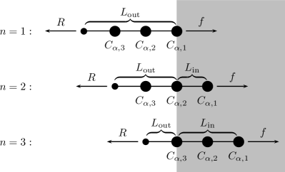
Figure 1: Illustration of our setup for $N=3$ and $n=1,2,3$. The portion of the chain outside the pore is represented, for simplicity only, in a fully extended configuration.

In [26], translocation of the green fluorescent protein (GFP) by a molecular motor was studied and quantitatively characterized by means of a single molecule experiment. Using suitable handles, the C–terminal of GFP was attached to the molecular motor ClpX (alone, or bound to the peptidase ClpP which degrades the translocated protein), while a resisting force was applied to the N–terminal by means of a suitable optical trap apparatus. ClpX was shown to exert a mechanical force to unfold GFP and translocate it in a stepwise fashion through its pore. Among other results, the translocation velocity was evaluated as a function of the resisting force, and it was shown that GFP unfolding is most often a 2–stage phenomenon, proceeding through an intermediate state.

In our study we shall focus on the above two aspects of this phenomenon, which can be easily described in the framework of our simple model: by studying the mean translocation time we shall show that it depends non–monotonically on the resisting force, while by simulating single trajectories we show that unfolding occurs through an intermediate state, which has the same structure observed in the experiment.

2 Model

The model has 2 sets of binary degrees of freedom. For a protein of $N$ aminoacids, we associate a variable $m_{k}$ to each aminoacid $k=1,\ldots N$, taking values $0,1$. $m_{k}=1(0)$ represents an aminoacid in a native–like (unfolded) configuration. Two aminoacids $i$ and $j>i$ can interact only if they are in contact in the native state and all aminoacids from $i$ to $j$ are native–like. Given a configuration $m=\{m_{k}\}$, an additional set $\sigma=\{\sigma_{ij}\}$ of binary variables is defined, which specifies the orientation of the protein chain with respect to an external force. More precisely, we associate an orientational variable $\sigma_{ij}=\pm 1$ to each portion of the chain delimited by two non–native aminoacids $i$ and $j>i$, such that $(1-m_{i})(1-m_{j})\prod_{k=i+1}^{j-1}m_{k}=1$. Given a reference direction (which in the following will be the direction of the forces acting on the protein), $\sigma_{ij}=+1$ (-1) means that the stretch from $i$ to $j$ is parallel (antiparallel) to the reference direction. Pictorially, we can think to the protein backbone as represented by the sequence of $C_{\alpha}$ atoms, divided into native–like stretches (which can be as short as the link between two consecutive $C_{\alpha}$’s and as long as the whole chain) that can rotate around the “unfolded” $C_{\alpha}$’s. Everything is then reduced to a 1–dimensional projection along the reference direction and the end–to–end lengths $\{l_{ij}\}$ of the native stretches are read from the Protein Data Bank (PDB).

In the present application to the translocation problem we consider a narrow, long and neutral pore, and introduce an additional degree of freedom, $n$, which specifies the position of the protein with respect to the pore. The portion of the chain from aminoacid 1 to $n$ is inside the pore, frozen in an unfolded, extended state, represented by the conditions $m_{k}=0\ (k=1,\ldots n)$ and $\sigma_{k,k+1}=+1\ (k=1,\ldots n-1)$. Physically, the pore is assumed to be (i) narrow, so that the protein must unfold and orient in the force direction to enter, (ii) sufficiently long to contain the whole protein, so that refolding is not possible after translocation (one might as well think that the protein has been degraded, as it can happen with the molecular motors studied in [26]), and (iii) neutral (no interaction with the protein except for the above–mentioned geometrical constraints). The remaining portion, from aminoacid $n+1$ to $N$, is outside the pore and its degrees of freedom can vary as described above.

The model can be defined through the following Hamiltonian:

$$H(m,\sigma,n)=-\epsilon\sum_{i=n+1}^{N-1}\sum_{j=i+1}^{N}\Delta_{ij}\prod_{k=i}^{j}m_{k}-fL_{\tx}{in}+RL_{\tx}{out}.$$ (1)

Here $\Delta$ is a contact matrix: its element $\Delta_{ij}$ is defined as the number of atomic contacts between aminoacids $i$ and $j$, where we have an atomic contact whenever 2 atoms (hydrogens excluded) are closer than 4 Å in the native configuration reported in the PDB. $\epsilon$ is the contact interaction energy, and all energies will be defined in units of $k_{B}T$, where $k_{B}$ is Boltzmann’s constant and $T$ absolute temperature. In the following we choose $\epsilon=0.13$, a value at which GFP (PDB code 1B9C, chain A) in absence of forces is fully native (the average fraction of native contacts is $Q=0.9827$, while the midpoint of the denaturation transition, where $Q=1/2$, corresponds to $\epsilon=0.116$).

The model contains also 2 force terms. $f$ is the importing force, exerted by the molecular motor. In the picture of a long pore, we can think that this force is applied to aminoacid number 1. Assuming that the pore position is fixed, this force is coupled to $L_{\tx}{in}=\sum_{i=1}^{n-1}l_{i,i+1}$, the length of the portion of the chain inside the pore. According to the so–called power–stroke scenario [25, 26], the actual force generated by the molecular motor is believed to be a time–dependent force, made of short pulses, and we can think that $f$ is the corresponding time average. $R$ is the resisting force, which in [26] was exerted by the optical tweezers apparatus. This is coupled to the length of the portion of the chain which is outside the pore,

$$L_{\tx}{out}=-\sum_{i=n}^{N}\sum_{j=i+1}^{N+1}l_{ij}\sigma_{ij}(1-m_{i})(1-m_{j})\prod_{k=i+1}^{j-1}m_{k},$$ (2)

with the boundary condition $m_{N+1}=0$ (an always unfolded variable is associated to the last atom of aminoacid number $N$, to which $R$ is applied). In the following we shall assume that $R$ is kept constant during the unfolding and translocation processes: several measurements were taken in [26] under this condition, which can be experimentally realized by means of a suitable feedback system.

As argued in [25], the conformational degrees of freedom, here represented by $m$ and $\sigma$, should have a much faster dynamics than the translational degree of freedom, here $n$. We therefore sum over $m$ and $\sigma$, obtaining the effective free energy

$$g(n)=-\ln\sum_{m,\sigma}\exp[-H(m,\sigma,n)],$$ (3)

where the sum can be evaluated in a numerically exact way by means of a polynomial (in $N$) recursive algorithm [16].

We use the above free energy to define a driven–diffusive dynamics for our model. At each time step, the number $n$ of imported aminoacids can vary by $\pm 1$ or 0. We have considered several choices for the transition probability, namely heat bath

$$W(n\to n+\Delta n)=\frac{\exp[-g(n+\Delta n)]}{\sum_{\Delta n^{\prime}=\pm 1,0}\exp[-g(n+\Delta n^{\prime})]},$$ (4)

which does not satisfy detailed balance, and 2 choices satisfying detailed balance, Metropolis and Glauber, where

$$W(n\to n\pm 1) = \frac{1}{2}w(g(n\pm 1)-g(n)),$$

$$W(n\to n) = 1-\sum_{\Delta n^{\prime}=\pm 1}W(n\to n+\Delta n^{\prime})$$ (5)

and $w(\Delta g)=\min(1,\exp(-\Delta g))$ for Metropolis, $w(\Delta g)=[1+\exp(\Delta g)]^{-1}$ for Glauber. The above rules are supplemented by suitable boundary conditions. We have an absorbing boundary at $n=N$, with $W(N\to N)=1$, $W(N\to N\pm 1)=0$, meaning that the translocation process is considered completed when all aminoacids have been imported into the pore. The boundary at $n=1$ is instead partially reflecting: in Eq. 4 $\Delta n=-1$ is forbidden and the normalization is modified accordingly, with similar changes for the Metropolis and Glauber choices. This means that in our model the protein cannot detach from the molecular motor.

Since we assume protein degrees of freedom are equilibrated during translocation events, our model should be more properly understood on a mesoscopic level rather than on a microscopic scale, the only one where dynamics is a priori expect to be reversible. This fact has stimulated us to consider a possible violation of detailed balance (heat bath) and to compare the corresponding kinetics with reversible evolutions (Metropolis and Glauber). However, this comparison has revealed that there is not any qualitative difference among such prescriptions within the present model, apart from the fact that heat bath is (roughly twice) faster than Metropolis, which in turn is faster than Glauber. As a consequence, the results reported below, which have been obtained with the heat bath dynamics, are rather robust.

Irrespectively of the choice of the dynamics, the evolution of the number $n$ of imported aminoacids is described by a simple stochastic process: a biased random walk on a lattice segment, with a partially reflecting and an absorbing boundary. Setting $n=1$ as our initial condition at time $t=0$, we define the translocation time $T$ as the first passage time at $n=N$: its average value will therefore be a mean first passage time, which can be evaluated by the generating function method [32], obtaining $\langle T\rangle=\sum_{n=1}^{N-1}\langle t\rangle_{n}$, where the average time spent at position $n$ is

$$\langle t\rangle_{n}=\frac{1}{W(n\to n+1)}\sum_{m=n}^{N-1}\prod_{l=m+1}^{n}\frac{W(l\to l-1)}{W(l\to l+1)}.$$ (6)

3 Results

We have evaluated the average translocation time $\langle T\rangle$ of GFP as a function of the importing force $f$, applied to the C–terminal, and the resisting force $R$, applied to the N–terminal. In Fig. 2 we report $\ln\langle T\rangle$ as a function of $f$ for several values of the resisting force $R$. In order to understand the content of the figure and the following discussion it is important to observe that both the time needed to unfold the molecule and the time needed to enter the pore contribute to $\langle T\rangle$.

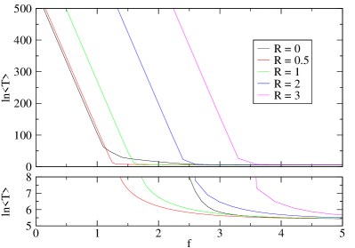
Figure 2: Logarithm of the translocation time $\langle T\rangle$ as a function of importing force and blow-up behavior at low $\ln\langle T\rangle$.

Two regimes are clearly observed. For small importing force, $\ln\langle T\rangle$ decreases linearly with $f$, consistently with Bell’s theory [33, 34] applied to mechanical unfolding in presence of a barrier. Indeed, in this regime, translocation is extremely slow because the importing force is not sufficient to overcome the free energy barrier to unfolding. As a consequence, $\langle T\rangle$ is dominated by the unfolding time.

For large importing force, $\ln\langle T\rangle$ is, on the scale of this graph, roughly independent on $f$. In this regime $f$ can easily unfold the protein, which can then enter the pore. However, as we shall see later, the average translocation time still depends on $f$ and $R$. It can be seen that for some values of the resisting force $R$ the transition between the 2 regimes occurs in 2 steps: this is the first signature we encounter of the presence of intermediates in GFP translocation (this is expected, since it is known that intermediates are found in GFP mechanical unfolding [35, 36]).

In Fig. 3 we report $1/\langle T\rangle$ as a function of the resisting force $R$ for different values of the importing force $f$. Several interesting phenomena can be observed. First of all, let us consider the $f=2$ curve. Even without resisting force, $R=0$, this importing force is too weak to unfold the protein and the inverse translocation time $1/\langle T\rangle$ (proportional to the translocation velocity) is practically zero on the scale of the graph: more precisely, this corresponds to the linearly decreasing branch in Fig. 2. Upon increasing $R$ we see that its effect is non–trivial: a small resisting force helps unfolding the protein, and after the unfolding the translocation becomes possible. Finally, by further increasing $R$, the translocation velocity decreases and eventually vanishes again. In this latter regime the protein is fully extended by the joint action of $f$ and $R$, and the translocation velocity is determined by the competition of these 2 forces.

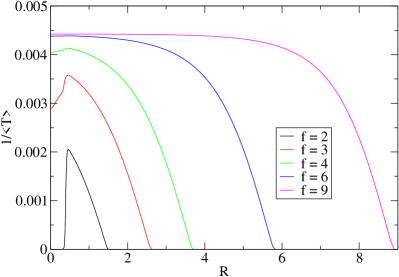
Figure 3: Inverse translocation time as a function of resisting force.

Increasing the importing force to $f=3$ we see that the translocation velocity is nonzero already at $R=0$ and for small increasing $R$ it grows up to a maximum. In this portion of the curve we can distinguish 2 regimes, separated by a change in slope. This is another signature of the presence of an intermediate: a small resisting force is more likely to unfold our protein only partially, while a larger $R$ can more easily give rise to complete unfolding.

The curve at $f=4$ can be qualitatively compared to the experimental results for the translocation velocity (which was measured in [26], see Fig. 2A, as a function of the resisting force): both exhibit a small increase at small $R$ and then a more or less sharp decrease at large $R$. Notice that our model cannot describe conformational fluctuations inside the pore, so we can compare, at least qualitatively, our results with the extension velocity in [26], but we cannot give an estimate of the contour velocity.

By increasing $f$ even further we see that the non–monotonicity disappears (the resisting force is no more needed to unfold the protein), the translocation speed saturates to $1/N$, meaning that the unfolding rate is so large that in most cases unfolding is immediate, and after that an aminoacid is imported at each time step. In this regime, the critical value of $R$ above which translocation is forbidden tends to $f$.

In the above results, forces and times have been reported in arbitrary units. The simplicity of the model is its strength, making it exactly solvable, but does not allow a full quantitative correspondence with the experimental results. At the order of magnitude level, we can say, by comparing our translocation velocity at saturation (large $f$, small $R$) with that reported in [26], that our time unit should be of order $10^{-2}$ s. Indeed, according to our setting, about $N/\langle T\rangle=1$ aminoacid per unit of time translocate at saturation, and this value must be identified with the maximum of 80 aminoacids per second found in [26]. On the other hand, it is known that this model fails to accurately predict forces quantitatively: see [17] for a discussion of this issue and of the need to introduce a suitable rescaling factor, and [20] where it is shown that the models can reproduce only qualitatively the hierarchy of GFP unfolding forces, when forces are applied in different directions. We therefore do not aim at a full quantitative discussion of force values and remain at the order of magnitude level: at this level, by observing that the GFP equilibrium unfolding force was reported [35] to be $\simeq 35$ pN, that the stall force in [26] was estimated to be around $20$ pN, and that the corresponding forces in our model are around a few units, we can estimate that our force unit should lie somewhere in between a few pN and 10 pN.

In order to better understand the nature of the intermediate state, we have simulated our stochastic process, generating single trajectories. In Fig. 4 we see a sample trajectory, obtained at $f=4,R=3.7$, which exhibits clearly the intermediate state. We chose these force values since the intermediate is short–lived, $\sim 0.18$ s in the experimental conditions [26], which corresponds roughly to $\sim 10$ time steps in our model. This is indeed the order of magnitude of the duration we observe at smaller resisting forces, and here we have chosen $f$ and $R$ almost balancing each other in order to extend the lifetime of the intermediate. This is a state with $n\simeq 95\div 110$ aminoacids inside the pore, which compares well to the intermediate with a C–terminal unfolded segment of length between 97 and 107 aminoacids observed in [26]. Structurally, this corresponds to unfolding and importing the 5 C–terminal $\beta$–strands, numbered 7–11, which are adjacent to each other in the native barrel structure, arranged in the order 11–10–7–8–9.

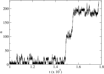
Figure 4: A sample trajectory showing the intermediate.

Although we cannot compare the corresponding result with experiments, we can easily check that if one reverses the protein, by applying $f$ to the N–terminal and $R$ to the C–terminal, a different intermediate is observed, with $n\sim 50$ imported aminoacids, corresponding to unfolding and importing the 3 N–terminal $\beta$–strands, numbered 1–3 and again adjacent to each other in the native barrel structure.

4 Conclusions

In the framework of an exactly solvable Ising–like model of protein thermal and mechanical (un)folding, we have shown how to obtain some exact nonequilibrium results by defining a diffusive dynamics on a suitable free energy profile. The dynamics was then reduced to a one–dimensional biased random walk on the corresponding reaction coordinate, which allowed to exactly compute mean first passage times and to easily simulate single trajectories. The approach can be applied to different situations, by choosing appropriate reaction coordinates, like the end–to–end length in the case of mechanical unfolding, or the number of contacts in the case of thermal or chemical (un)folding. Here, as an illustration, we chose the problem of the translocation of the green fluorescent protein through a narrow, long and neutral pore, under the action of an importing and a resisting force. The natural reaction coordinate in this case is the number of aminoacids imported into the pore. Our analysis focused on two aspects of the phenomenon, which can be described at the level of our extremely simplified model. The mean translocation time was exactly computed as a function of the forces, showing an interesting non–monotonic dependence on the resisting force, consistent with recent experimental observations [26]. Simulating single trajectories of our random walk, we have found evidences of a two–stage unfolding phenomenon, with an intermediate state whose number of imported aminoacids, and hence structure, are the same observed in the experiment [26].

References

- [1] \NameZimm B. Bragg J. \REVIEWJ. Chem. Phys.311959526.
- [2] \NamePoland D. Scheraga H. \REVIEWJ. Chem. Phys.4519661464.
- [3] \NameWako H. Saitô N. \REVIEWJ. Phys. Soc. Jpn4419781931.
- [4] \NameWako H. Saitô N. \REVIEWJ. Phys. Soc. Jpn4419781939.
- [5] \NameMuñoz V., Thompson P. A., Hofrichter J. Eaton W. A. \REVIEWNature3901997196.
- [6] \NameMuñoz V., Henry E. R., Hofrichter J. Eaton W. A. \REVIEWProc. Natl. Acad. Sci. USA9519985872.
- [7] \NameGalzitskaya O. Finkelstein A. \REVIEWProc. Natl. Acad. Sci. USA96199911299.
- [8] \NameAlm E. Baker D. \REVIEWProc. Natl. Acad. Sci. USA96199911305.
- [9] \NameMuñoz V. Eaton W. A. \REVIEWProc. Natl. Acad. Sci. USA96199911311.
- [10] \NameFlammini A., Banavar J. Maritan A. \REVIEWEurophys. Lett.582002623.
- [11] \NameBruscolini P. Pelizzola A. \REVIEWPhys. Rev. Lett.882002258101.
- [12] \NamePelizzola A. \REVIEWJ. Stat. Mech.2005P11010.
- [13] \NameBruscolini P., Pelizzola A. Zamparo M. \REVIEWPhys. Rev. Lett.992007038103.
- [14] \NameZamparo M. \REVIEWJ. Stat. Mech.2008P10013.
- [15] \NameImparato A., Pelizzola A. Zamparo M. \REVIEWPhys. Rev. Lett.982007148102.
- [16] \NameImparato A., Pelizzola A. Zamparo M. \REVIEWJ. Chem. Phys.1272007145105.
- [17] \NameImparato A. Pelizzola A. \REVIEWPhys. Rev. Lett.1002008158104.
- [18] \NameImparato A., Pelizzola A. Zamparo M. \REVIEWPhys. Rev. Lett.1032009188102.
- [19] \NameCaraglio M., Imparato A. Pelizzola A. \REVIEWJ. Chem. Phys.1332010065101.
- [20] \NameCaraglio M., Imparato A. Pelizzola A. \REVIEWPhys. Rev. E842011021918.
- [21] \NameAioanei D., Brucale M., Tessari I., Bubacco L. SamoríB. \REVIEWBiophys. J.1022012342.
- [22] \NameKenniston J. A., Baker T. A., Fernandez J. M. Sauer R. T. \REVIEWCell1142003511.
- [23] \NameKenniston J. A., Baker T. A. Sauer R. T. \REVIEWProc. Natl. Acad. Sci. USA10220051390.
- [24] \NameMartin A., Baker T. A. Sauer R. T. \REVIEWNat. Struct. Mol. Biol.1520081147.
- [25] \NameAubin-Tam M.-E., Olivares A. O., Sauer R. T., Baker T. A. Lang M. J. \REVIEWCell1452011257.
- [26] \NameMaillard R. A., Chistol G., Sen M., Righini M., Tan J., Kaiser C. M., Hodges C., Martin A. Bustamante C. \REVIEWCell1452011459.
- [27] \NameHuang L., Kirmizialtin S. Makarov D. E. \REVIEWJ. Chem. Phys.1232005124903.
- [28] \NameKirmizialtin S., Huang L. Makarov D. E. \REVIEWPhys. Stat. Sol. B24320062038.
- [29] \NameAmmenti A., Cecconi F., Marini Bettolo Marconi U. Vulpiani A. \REVIEWJ. Phys. Chem. B113200910348.
- [30] \NameChinappi M., Cecconi F. Casciola C. M. \REVIEWPhil. Mag.9120112034.
- [31] \NameKravats A., Jayasinghe M. Stan G. \REVIEWProc. Natl. Acad. Sci. USA10820112234.
- [32] \NameFeller W. \BookAn Introduction to Probability Theory and Its Applications, vol. 2 (Wiley, New York) 1966.
- [33] \NameBell G. \REVIEWScience2001978618.
- [34] \NameKumar S. Li M. \REVIEWPhys. Rep.48620101.
- [35] \NameDietz H. Rief M. \REVIEWProc. Natl. Acad. Sci. USA101200416192.
- [36] \NameMickler M., Dima R., Dietz H., Hyeon C., Thirumalai D. Rief M. \REVIEWProc. Natl. Acad. Sci. USA104200720268.