Estimating the mass of the hidden charm $1^{+}(1^{+})$ tetraquark state via QCD sum rules

Abstract

By using QCD sum rules, the mass of the hidden charm tetraquark $[cu][\bar{c}\bar{d}]$ state with $I^{G}(J^{P})=1^{+}(1^{+})$ (HCTV) is estimated, which presumably will turn out to be the newly observed charmonium-like resonance $Z_{c}^{+}(3900)$. In the calculation, contributions up to dimension eight in the operator product expansion(OPE) are taken into account. We find $m_{1^{+}}^{c}=(3912^{+306}_{-153})\,\text{MeV}$, which is consistent, within the errors, with the experimental observation of $Z_{c}^{+}(3900)$. Extending to the b-quark sector, $m_{1^{+}}^{b}=(10561^{+395}_{-163})\,\text{MeV}$ is obtained. The calculational result strongly supports the tetraquark picture for the “exotic” states of $Z_{c}^{+}(3900)$ and $Z_{b}^{+}(10610)$.

1 Introduction

Recently, the BESIII Collaboration reported the observation of a new charged charmonium-like state in the $J/\psi\pi^{\pm}$ channel in $Y(4260)\rightarrow J/\psi\pi^{+}\pi^{-}$ decay [1]. Its mass and width are $(3899.0\pm 3.6\pm 4.9)\,\text{MeV}$ and $(46\pm 10\pm 20)\,\text{MeV}$, respectively. Soon afterwards, the Belle [2] and CLEO [3] Collaborations confirmed the existence of this hadronic structure. Notice that this new resonance, nominated as $Z_{c}^{+}(3900)$, is a charged charmonium-like state; therefore, it certainly contains at least four quarks, a pair of charm quarks and two light quarks. It is an exotic state. In the b-quark sector, recall that two bottom-like charged sates $Z_{b}^{+}(10610)$ and $Z_{b}^{+}(10650)$ were observed by the Belle Collaboration [4, 5]. That implies that there exist similar structures in the charm and bottom energy regions. These new findings reflect the renaissance of the study of the so-called exotic states.

In the literature, various models have been proposed to interpret the new experimental observations. For $Z_{c}^{+}(3900)$, for instance, models of the molecular state [6, 7, 8, 9, 10], the tetraquark state [11, 12, 13], the initial single pion emission (ISPE) scheme [14] and so on were proposed. For a comprehensive review of the theoretical status of this state, we refer the reader to Ref.[15]. Since a definite conclusion has not yet been reached, more efforts are still necessary to explore its inner structure.

The method of QCD sum rules [16, 17, 18, 19] has been applied successfully to many hadronic phenomena, such as the hadron spectrum and hadron decays. In this approach, an interpolating current with proper quantum numbers are constructed corresponding to a hadron of interest. Then, by constructing a correlation function and matching its operator product expansion (OPE) to its hadronic saturation, the main function for extracting the mass or decay rate of the hadron is established. In the original paper on the quark model [20], Gell-Mann discussed the possibility of the existence of free diquarks. The concept of diquark is based on the fundamental theory, and has been invoked to interpret a number of phenomena observed in experiment [21, 22, 23]. In Ref.[24], the exotic state X(3872) was explored through the QCD sum rules, where the hadronic state was considered as a hidden charm tetraquark state with quantum number $I^{G}(J^{PC})=0^{+}(1^{++})$ (HCTS). Employing the same interpolating current, Chen and Zhu investigated the $1^{+-}$ tetraquark state and found its mass to be $(4.02\pm 0.09)\,\text{GeV}$ [25].

In this paper, we calculate the mass of the hidden charm tetraquark state with $I^{G}(J^{P})=1^{+}(1^{+})$ (HCTV) by using the QCD sum rules, and confront it with the $Z_{c}^{+}(3900)$. Here, the HCTV is interpreted as the isospin 1 partner of the HCTS. Comparing this work with Ref.[24], two differences are noteworthy. First, the interpolating current here is different from the HCTS current. Second, of the HCTV, as mentioned in Ref.[24], the higher-dimensional two-gluon and mixed condensates are not negligible in order to obtain a reasonable sum rule. Hence, in this work, the non-perturbative condensates up to dimension eight are taken into account. In addition, different from Refs.[24, 25, 26] on HCTV, in our analysis the quark-gluon condensate term in the light-quark “full” propagator is considered, and a moderate criterion is adopted in finding the available threshold parameter $\sqrt{s_{0}}$ and the Borel window $M_{B}^{2}$.

2 Formalism

The starting point of the QCD sum rules is the two-point correlation function constructed from the interpolating current:

$$\Pi_{\mu\nu}(q)=i\int d^{4}xe^{iq\cdot x}\langle 0|T\big{\{}j_{\mu}(x)j^{\dagger}_{\nu}(0)\big{\}}|0\rangle\;.$$ (1)

The interpolating current of the HCTV is expressed as [12]:

$$j_{\mu}(x)=\frac{i\epsilon_{abc}\epsilon_{dec}}{\sqrt{2}}\big{[}\left(u^{T}_{a}(x)C\gamma_{5}c_{b}(x)\right)\left(\bar{d}_{d}\gamma_{\mu}C\bar{c}_{e}^{T}\right)-\left(u^{T}_{a}(x)C\gamma_{\mu}c_{b}(x)\right)\left(\bar{d}_{d}\gamma_{5}C\bar{c}_{e}^{T}\right)\big{]}\;,$$ (2)

where $a$, $b$, $c$, $\cdots$, are color indices, and $C$ represents the charge conjugation matrix. Note that there is a minus sign difference between the current given in Eq.(2) and the one in Ref.[24]. Therefore, even under the SU(2) symmetry the mass obtained for the HCTV differs from the HCTS, which is what is to be analyzed in the following.

Generally, the two-point correlation function takes the following Lorentz covariance form:

$$\Pi_{\mu\nu}(q)=-\left(g_{\mu\nu}-\frac{q_{\mu}q_{\nu}}{q^{2}}\right)\Pi_{1}(q^{2})+\frac{q_{\mu}q_{\nu}}{q^{2}}\Pi_{0}(q^{2})\;.$$ (3)

Because the axial vector current is not conserved, there are two independent parts appearing in the correlation function, i.e. $\Pi_{1}(q^{2})$ and $\Pi_{0}(q^{2})$, where the subscripts 1 and 0 denote the quantum numbers of the spin 1 and 0, respectively.

On the phenomenological side, after separating the ground state contribution from the pole term in $\Pi_{1}(q^{2})$, the correlation function is expressed as a dispersion integral over a physical regime, i.e.,

$$\Pi_{1}(q^{2}) = \frac{\lambda_{1^{+}}^{c\;2}}{m_{1^{+}}^{c\;2}-q^{2}}+\frac{1}{\pi}\int_{s_{0}}^{\infty}ds\frac{\rho^{h}(s)}{s-q^{2}}\;.$$ (4)

Here, $m_{1^{+}}^{c}$ represents the HCTV mass, $\rho^{h}(s)$ is the spectral density representing the contributions of higher excited and continuum states, $s_{0}$ denotes the threshold of higher excited and continuum states, and $\lambda_{1^{+}}^{c}$ stands for the pole residue, representing the coupling strength defined by $\langle 0|j_{\mu}|\text{HCTV}\rangle=\lambda_{1^{+}}^{c}\epsilon_{\mu}$.

On the OPE side of $\Pi_{1}(q^{2})$, the correlation function can be expressed as a dispersion relation:

$$\Pi_{1}^{OPE}(q^{2})=\int_{4m_{c}^{2}}^{\infty}ds\frac{\rho^{OPE}(s)}{s-q^{2}}+\Pi_{1}^{\langle g_{s}\bar{q}\sigma\cdot Gq\rangle\langle\bar{q}q\rangle}(q^{2})+\Pi_{1}^{\langle g_{s}^{2}G^{2}\rangle^{2}}(q^{2})\;.$$ (5)

Here, $\rho^{OPE}$ is given by the imaginary part of the correlation function, $\rho^{OPE}(s)=\text{Im}[\Pi_{1}^{OPE}(s)]/{\pi}$ and it can be written as

$$\rho^{OPE}(s) = \rho^{pert}(s)+\rho^{\langle\bar{q}q\rangle}(s)+\rho^{\langle g_{s}^{2}G^{2}\rangle}(s)+\rho^{\langle g_{s}\bar{q}\sigma\cdot Gq\rangle}(s)+\rho^{\langle\bar{q}q\rangle^{2}}(s)+\rho^{\langle g_{s}^{3}G^{3}\rangle}(s)$$ (6)

$$+ \rho^{\langle g_{s}\bar{q}\sigma\cdot Gq\rangle\langle\bar{q}q\rangle}(s)+\rho^{\langle g_{s}^{2}G^{2}\rangle^{2}}+\cdots\;,$$

where “$\cdots$” stands for other higher dimension condensates neglected in this work. $\Pi_{1}^{\langle g_{s}\bar{q}\sigma\cdot Gq\rangle\langle\bar{q}q\rangle}(q^{2})$ and $\Pi_{1}^{\langle g_{s}^{2}G^{2}\rangle^{2}}(q^{2})$ denote those contributions of the correlation function which have no imaginary parts but have nontrivial values under the Borel transform. After making the Borel transform on the OPE side, we get

$$\Pi_{1}^{OPE}(M_{B}^{2})=\int_{4m_{c}^{2}}^{\infty}ds\rho^{OPE}(s)e^{-s/M_{B}^{2}}+\Pi_{1}^{\langle g_{s}\bar{q}\sigma\cdot Gq\rangle\langle\bar{q}q\rangle}(M_{B}^{2})+\Pi_{1}^{\langle g_{s}^{2}G^{2}\rangle^{2}}(M_{B}^{2})\;.$$ (7)

To evaluate the spectral density, the “full” propagators $S^{q}_{ij}(x)$ and $S^{Q}_{ij}(p)$ for light ($q=u$, $d$ or $s$) and heavy quarks ($Q=c$ or $b$) are necessary, in which the vacuum condensates are explicitly shown [17], i.e.,

$$S^{q}_{ij}(x)\!\!\! = \!\!\!\frac{i\delta_{ij}\hat{x}}{2\pi^{2}x^{4}}-\frac{m_{q}\delta_{ij}}{4\pi^{2}x^{2}}-\frac{ig_{s}t^{a}_{ij}G^{a}_{\kappa\lambda}}{32\pi^{2}x^{2}}(\sigma^{\kappa\lambda}\hat{x}+\hat{x}\sigma^{\kappa\lambda})+\frac{i\delta_{ij}\hat{x}}{48}m_{q}\langle\bar{q}q\rangle-\frac{\delta_{ij}\langle\bar{q}q\rangle}{12}$$ (8)

$$- \!\!\!\frac{\delta_{ij}\langle g_{s}\bar{q}\sigma Gq\rangle x^{2}}{192}-\frac{t^{a}_{ij}\sigma^{\kappa^{\prime}\lambda^{\prime}}}{192}\langle g_{s}\bar{q}\sigma\cdot G^{\prime}q\rangle+\cdots\;,$$

$$S^{Q}_{ij}(p)\!\!\! = \!\!\!\int\frac{d^{4}p}{(2\pi)^{4}}e^{-ip\cdot x}\bigg{\{}\frac{i}{\hat{p}-m_{Q}}\delta_{ij}-\frac{i}{4}g_{s}(t^{c})_{ij}G^{c}_{\kappa\lambda}\frac{1}{(p^{2}-m_{Q}^{2})^{2}}$$ (9)

$$\times \!\!\![\sigma^{\kappa\lambda}(\hat{p}+m_{Q})+(\hat{p}+m_{Q})\sigma^{\kappa\lambda}]+\frac{i}{12}g_{s}^{2}\delta_{ij}G^{a}_{\alpha\beta}G^{a}_{\alpha\beta}m_{Q}\frac{p^{2}+m_{Q}\hat{p}}{(p^{2}-m_{Q}^{2})^{4}}$$

$$+ \!\!\!\frac{i\delta_{ij}}{48}\bigg{[}\frac{(\hat{p}+m_{Q})[\hat{p}(p^{2}-3m_{Q}^{2})+2m_{Q}(2p^{2}-m_{Q}^{2})](\hat{p}+m_{Q})}{(p^{2}-m_{Q}^{2})^{6}}\bigg{]}\langle g_{s}^{3}G^{3}\rangle+\cdots\bigg{\}}\;.$$

Here, $G^{\prime}$ represents the outer gluon field and the Lorentz indices $\kappa^{\prime}$ and $\lambda^{\prime}$ are indices of the outer gluon field coming from another propagator [27].

We calculate the spectral density $\rho^{OPE}(s)$ up to dimension eight at the leading order in $\alpha_{s}$ by the standard technique of QCD sum rules. In order to find the difference between HCTV and HCTS, we keep not only terms linear in the light-quark masses $m_{u}$ and $m_{d}$, but also the two-gluon and the quark-gluon mixed condensates up to dimension eight. Through a lengthy calculation, the spectral densities on the OPE side are obtained as:

$$\rho^{pert}(s)\!\!\! = \!\!\!\frac{1}{2^{10}\pi^{6}}\int^{\alpha_{max}}_{\alpha_{min}}\frac{d\alpha}{\alpha^{3}}\int^{1-\alpha}_{\beta_{min}}\frac{d\beta}{\beta^{3}}(1-\alpha-\beta)(1+\alpha+\beta){\cal F}(\alpha,\beta,s)^{4}$$ (10)

$$+ \!\!\!\frac{(m_{u}+m_{d})m_{c}}{2^{9}\pi^{6}}\int^{\alpha_{max}}_{\alpha_{min}}\frac{d\alpha}{\alpha^{2}}\int^{1-\alpha}_{\beta_{min}}\frac{d\beta}{\beta^{3}}(\alpha+\beta-1)(3+\alpha+\beta){\cal F}(\alpha,\beta,s)^{3}\;,$$

$$\rho^{\langle\bar{q}q\rangle}(s)\!\!\! = \!\!\!-\frac{m_{c}\langle\bar{q}q\rangle}{2^{5}\pi^{4}}\int^{\alpha_{max}}_{\alpha_{min}}\frac{d\alpha}{\alpha^{2}}\int^{1-\alpha}_{\beta_{min}}\frac{d\beta}{\beta}(1+\alpha+\beta){\cal F}(\alpha,\beta,s)^{2}$$ (11)

$$+ \!\!\!\frac{(m_{u}+m_{d})\langle\bar{q}q\rangle}{2^{6}\pi^{4}}\bigg{[}\int_{\alpha_{min}}^{\alpha_{max}}\frac{d\alpha}{\alpha(1-\alpha)}{\cal H}(\alpha,s)^{2}-\int^{\alpha_{max}}_{\alpha_{min}}\frac{d\alpha}{\alpha}\int^{1-\alpha}_{\beta_{min}}\frac{d\beta}{\beta}{\cal F}(\alpha,\beta,s)^{2}$$

$$+ \!\!\!4m_{c}^{2}\int^{\alpha_{max}}_{\alpha_{min}}\frac{d\alpha}{\alpha}\int^{1-\alpha}_{\beta_{min}}\frac{d\beta}{\beta}{\cal F}(\alpha,\beta,s)\bigg{]}\;,$$

$$\rho^{\langle g_{s}^{2}G^{2}\rangle}(s)\!\!\! = \!\!\!\frac{\langle g_{s}^{2}G^{2}\rangle}{3\times 2^{9}\pi^{6}}\int^{\alpha_{max}}_{\alpha_{min}}\!\!\!d\alpha\int^{1-\alpha}_{\beta_{min}}\!\!\frac{d\beta}{\beta^{2}}\bigg{[}\frac{m_{c}^{2}(1-(\alpha+\beta)^{2})}{\beta}-\frac{(1-2\alpha-2\beta)}{2\alpha}{\cal F}(\alpha,\beta,s)\bigg{]}$$ (12)

$$\times \!\!\!{\cal F}(\alpha,\beta,s)-\frac{m_{c}^{2}\langle g_{s}^{2}G^{2}\rangle}{3\times 2^{12}\pi^{6}}\int^{\alpha_{max}}_{\alpha_{min}}\frac{d\alpha}{\alpha}\int^{1-\alpha}_{\beta_{min}}\frac{d\beta}{\beta}\bigg{[}(1+\alpha+\beta)$$

$$\times \!\!\!-\frac{(1-\alpha-\beta)(\alpha+\beta+3)}{\alpha}+\frac{1}{4\alpha\beta}(\alpha+\beta-1)^{2}(\alpha+\beta+5)\bigg{]}{\cal F}(\alpha,\beta,s)\;,$$

$$\rho^{\langle g_{s}\bar{q}\sigma\cdot Gq\rangle}(s)\!\!\! = \!\!\!-\frac{m_{c}\langle g_{s}\bar{q}\sigma\cdot Gq\rangle}{2^{6}\pi^{4}}\bigg{[}2\int^{\alpha_{max}}_{\alpha_{min}}\frac{d\alpha}{\alpha}{\cal H}(\alpha,s)-\int^{\alpha_{max}}_{\alpha_{min}}\!\!\!d\alpha\int^{1-\alpha}_{\beta_{min}}\!\!\!d\beta\left(\frac{1}{\alpha}+\frac{\alpha+\beta}{\beta^{2}}\right)$$ (13)

$$\times \!\!\!{\cal F}(\alpha,\beta,s)\bigg{]}+\frac{m_{c}\langle g_{s}\bar{q}\sigma\cdot Gq\rangle}{3\times 2^{8}\pi^{4}}\int^{\alpha_{max}}_{\alpha_{min}}\frac{d\alpha}{\alpha}\bigg{[}2{\cal H}(\alpha,s)$$

$$- \!\!\!\int^{1-\alpha}_{\beta_{min}}d\beta\left(1+\frac{(1+\alpha+\beta)}{\alpha}\right){\cal F}(\alpha,\beta,s)\bigg{]}\;,$$

$$\rho^{\langle\bar{q}q\rangle^{2}}(s)\!\!\! = \!\!\!\frac{\langle\bar{q}q\rangle^{2}}{12\pi^{2}}m_{c}^{2}\sqrt{1-4m_{c}^{2}/s}\;,$$ (14)

$$\rho^{\langle g_{s}^{3}G^{3}\rangle}(s)\!\!\! = \!\!\!\frac{\langle g_{s}^{3}G^{3}\rangle}{3\times 2^{10}\pi^{6}}\int^{\alpha_{max}}_{\alpha_{min}}d\alpha\int^{1-\alpha}_{\beta_{min}}\frac{d\beta}{\beta^{3}}(1-\alpha-\beta)(1+\alpha+\beta)$$ (15)

$$\times \!\!\!\bigg{[}m_{c}^{2}\alpha+\frac{{\cal F}(\alpha,\beta,s)}{2}\bigg{]}\;,$$

$$\rho^{\langle g_{s}\bar{q}\sigma\cdot Gq\rangle\langle\bar{q}q\rangle}(s)\!\!\! = \!\!\!-\frac{\langle g_{s}\bar{q}\sigma\cdot Gq\rangle\langle\bar{q}q\rangle}{3^{2}\times 2^{5}\pi^{2}}\int^{\alpha_{max}}_{\alpha_{min}}\alpha d\alpha\;,$$ (16)

$$\rho^{\langle g_{s}^{2}G^{2}\rangle^{2}}(s)\!\!\! = \!\!\!-\frac{23\langle g_{s}^{2}G^{2}\rangle^{2}}{3^{3}\times 2^{16}\pi^{6}}\bigg{[}\int^{\alpha_{max}}_{\alpha_{min}}d\alpha\int^{1-\alpha}_{\beta_{min}}d\beta+\int^{\alpha_{max}}_{\alpha_{min}}d\alpha\bigg{]}\;,$$ (17)

and

$$\Pi_{1}^{\langle g_{s}\bar{q}\sigma\cdot Gq\rangle\langle\bar{q}q\rangle}(M_{B}^{2})\!\!\! = \!\!\!-\frac{m_{c}^{2}\langle g_{s}\bar{q}\sigma\cdot Gq\rangle\langle\bar{q}q\rangle}{24\pi^{2}}\int^{1}_{0}d\alpha\bigg{[}1+\frac{m_{c}^{2}}{\alpha(1-\alpha)M_{B}^{2}}$$ (18)

$$- \!\!\!\frac{5}{12(1-\alpha)}\bigg{]}e^{-\frac{m_{c}^{2}}{\alpha(1-\alpha)M_{B}^{2}}}\;,\;\;\;\;\;\;\;\;\;\;$$

$$\Pi_{1}^{\langle g_{s}^{2}G^{2}\rangle^{2}}(M_{B}^{2})\!\!\! = \!\!\!-\frac{11m_{c}^{2}\langle g_{s}^{2}G^{2}\rangle^{2}}{3^{2}\times 2^{18}\pi^{6}}\int_{0}^{1}d\alpha\int_{0}^{1-\alpha}d\beta\frac{(1-\alpha-\beta)}{\alpha\beta}e^{-\frac{(\alpha+\beta)m_{c}^{2}}{\alpha\beta M_{B}^{2}}}$$ (19)

$$+ \!\!\!\frac{m_{c}^{4}\langle g_{s}^{2}G^{2}\rangle^{2}}{3^{3}\times 2^{14}\pi^{6}}\left(1+\frac{1}{M_{B}^{2}}\right)\int_{0}^{1}\frac{d\alpha}{\alpha^{3}}\int_{0}^{1-\alpha}\frac{d\beta}{\beta^{3}}\bigg{[}-\frac{(\alpha^{2}+\beta^{2})(1-\alpha-\beta)^{2}}{4}$$

$$- \!\!\!\frac{(\alpha^{3}+\beta^{3})}{2}+(1-\alpha-\beta)(\alpha^{3}+2\alpha^{2}+2\beta^{2}+\beta^{3})\bigg{]}e^{-\frac{(\alpha+\beta)m_{c}^{2}}{\alpha\beta M_{B}^{2}}}\;.$$

Here, $M_{B}$ is the Borel parameter introduced by the Borel transform; we have the functions ${\cal F}(\alpha,\beta,s)=(\alpha+\beta)m_{c}^{2}-\alpha\beta s$ and ${\cal H}(\alpha,s)=m_{c}^{2}-\alpha(1-\alpha)s$; the integration bounds are $\alpha_{min}=(1-\sqrt{1-4m_{c}^{2}/s})/2$, $\alpha_{max}=(1+\sqrt{1-4m_{c}^{2}/s})/2$ and $\beta_{min}=\alpha m_{c}^{2}/(s\alpha-m_{c}^{2})$.

Matching the OPE side expression of the correlation function $\Pi_{1}(q^{2})$ with the phenomenological side one, and performing the Borel transform, one obtains a sum rule for the corresponding HCTV mass. It reads

$$m_{1^{+}}^{c}(s_{0},M_{B}^{2})=\sqrt{-\frac{R_{1}(s_{0},M_{B}^{2})}{R_{0}(s_{0},M_{B}^{2})}}\;$$ (20)

with

$$R_{0}(s_{0},M_{B}^{2}) = \int_{4m_{c}^{2}}^{s_{0}}ds\;\rho^{OPE}(s)e^{-s/M_{B}^{2}}+\Pi_{1}^{\langle g_{s}\bar{q}\sigma\cdot Gq\rangle\langle\bar{q}q\rangle}(M_{B}^{2})+\Pi_{1}^{\langle g_{s}^{2}G^{2}\rangle^{2}}(M_{B}^{2})\;,$$ (21)

$$R_{1}(s_{0},M_{B}^{2}) = \frac{\partial}{\partial{M_{B}^{-2}}}{R_{0}(s_{0},M_{B}^{2})}\;.$$ (22)

It should be mentioned that in principle the four-gluon operator, the $\langle g_{s}^{2}G^{2}\rangle^{2}$, also belongs to the dimension-eight condensate, however, in practice we find it is only 1 % of the mixed condensate $\langle g_{s}\bar{q}\sigma\cdot Gq\rangle\langle\bar{q}q\rangle$ in magnitude, and hence the four-gluon condensate is neglected in the evaluation of this work. Moreover, in order to obtain a relatively reliable result through the leading order calculation, one needs to depress the higher order QCD corrections and hence to express the $m_{1^{+}}^{c}$ in terms of Eq.(20), which is found to be less sensitive to the radiative corrections than to the individual moments [24].

3 Numerical Analysis

In performing the numerical evaluation, the values of the input parameters, the condensates, and the quark masses are adopted as follows [24, 26, 28, 29]:

$$\begin{aligned} &m_{u}=2.3\;\text{MeV}\;,&&m_{d}=6.4\;\text{MeV}\;,\\ &m_{c}(m_{c})=(1.23\pm 0.05)\;\text{GeV}\;,&&m_{b}(m_{b})=(4.24\pm 0.06)\;\text{GeV},\\ &\langle\bar{q}q\rangle=-(0.23\pm 0.03)^{3}\;\text{GeV}^{3}\;,&&\langle g_{s}^{2}G^{2}\rangle=0.88\;\text{GeV}^{4}\;,\\ &\langle\bar{q}g_{s}\sigma\cdot Gq\rangle=m_{0}^{2}\langle\bar{q}q\rangle\;,&&\langle g_{s}^{3}G^{3}\rangle=0.045\;\text{GeV}^{6}\;,\\ &m_{0}^{2}=0.8\;\text{GeV}^{2}\;.&&\end{aligned}$$ (23)

Here, the scale dependence of these parameters is not taken into account since our calculation is performed at the leading order in $\alpha_{s}$. The quark masses used here are evaluated in Ref. [29] by virtue of the QCD sum rules and hence they are defined in the $\overline{\rm MS}$-scheme. For more details of the nature of the inputs, one may refer to Ref.[24].

In the approach of QCD sum rules, choosing a proper threshold $s_{0}$ and Borel parameter $M_{B}^{2}$ are critical to obtain a reasonable result. There are two criteria in making such choices [16, 17, 19]. First, the convergence of the OPE should be kept. To this aim, one may compare the relative contribution of each term in Eqs.(10) to (19) with the total contribution on the OPE side, which are shown in Fig.1. From the figure, we notice that a quite good OPE convergence occurs when $M_{B}^{2}\geq 1.9\;\text{GeV}^{2}$, and then we fix the lower working limit for $M_{B}^{2}$.

Figure 1: The OPE convergence in the region $1.6\leq M_{B}^{2}\leq 3.0\,\text{GeV}^{2}$ at $\sqrt{s_{0}}=4.15\,\text{GeV}$. The solid line denotes the fraction of the perturbative contribution, and each subsequent line denotes the addition of one extra condensate dimension in the expansion, i.e., $\langle\bar{q}q\rangle$ (short-dashed line), $\langle g_{s}^{2}G^{2}\rangle$ (dotted line), $\langle g_{s}\bar{q}\sigma\cdot Gq\rangle$ (dotted-dashed line), and $\langle\bar{q}q\rangle^{2}$ (long-dashed line)

The second criterion to constrain the $M_{B}^{2}$ is that the pole contribution should be larger than the continuum contribution. That means we need to evaluate the relative pole contribution (PC) to the total, the pole plus continuum, for various values of $M_{B}^{2}$. To eliminate the contributions from the higher excited and continuum states properly, we ask the pole contribution to be larger than $50\%$ [19, 24], which is a little different from the constraint in [25]. The relative weight is presented in Fig.2, which tells the upper limit for $M_{B}^{2}$. We note that the upper constraint on $M_{B}^{2}$ depends on the threshold value $s_{0}$. So, for different $s_{0}$, we will find different upper bounds for $M_{B}^{2}$. To determine the proper value of $s_{0}$, we carry out a similar analysis to Ref.[24], and find that the optimal value of $s_{0}$ obtained there is also suitable in our case. The reason is that the dominant contributions of the OPE side are the same in this work and Ref.[24]. Thus, for the proper $s_{0}$ in our analysis, $\sqrt{s_{0}}=4.15\;\text{GeV}$, we find $M_{B}^{2}\leq 2.3\text{GeV}^{2}$.

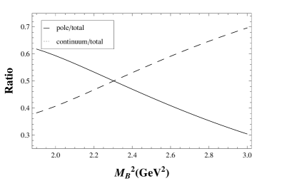
Figure 2: The relative pole and continuum contributions at $\sqrt{s_{0}}=4.15\;\text{GeV}$. The solid line represents the relative pole contribution, and the dashed line corresponds to the relative continuum contribution

Since the interpolating current in Eq.(2) is different from what in Ref.[24], the OPE contributions in this work and in the HCTS analysis must be different. To highlight the contributions of the new high-dimensional condensates in the HCTV, in Table.1 we present the relative ratios of the additional terms to the existing terms in Ref.[24] for each involved condensate at $\sqrt{s_{0}}=4.15\;\text{GeV}$. Among these ratios in Table.1, we find that the additional contributions of dimension-four and -eight condensates are considerable for the HCTV, which is different from the case in Ref.[24]. That is to say, the inclusion of high-dimensional condensates is necessary in obtaining a precise and reliable mass of the HCTV. Fig.3 shows the dependence of $m_{1^{+}}^{c}$ on the Borel parameter $M_{B}^{2}$, where lines from bottom to top correspond to the continuum threshold $\sqrt{s_{0}}$ being $4.05$, $4.15$, $4.25\,\text{GeV}$, respectively.

Table 1: The relative ratios of the additional terms to those terms in Ref.[24] at $\sqrt{s_{0}}=4.15\;\text{GeV}$. The subscripts denote the condensate dimensions. The “$\text{ratio}_{O_{4}}$” denotes the ratio of the second term to the first term in Eq.(12); the “$\text{ratio}_{O_{5}}$” denotes the second term to the first term in Eq.(13); “$\text{ratio}_{O_{6}}$” for Eq.(15) to Eq.(14); and “$\text{ratio}_{O_{8}}$” for Eq.(16) to Eq.(18), respectively

$M_{B}^{2}(\text{GeV}^{2})$	1.6	1.9	2.2	2.5	2.8
$\text{ratio}_{O_{4}}$	0.45	0.39	0.34	0.31	0.29
$\text{ratio}_{O_{5}}$	0.03	0.03	0.03	0.04	0.04
$\text{ratio}_{O_{6}}$	$<0.01$	0.01	0.01	0.01	0.01
$\text{ratio}_{O_{8}}$	0.06	0.07	0.08	0.10	0.11

In the end, we obtain the HCTV mass:

$$m_{1^{+}}^{c}=(3912^{+306}_{-153})\,\text{MeV}\;.$$ (24)

Here, the errors stem from the uncertainties of the Borel parameter $M_{B}$, the charm quark mass, the condensates, and the threshold parameter $s_{0}$. Note that the difference between the upper error and the lower error is due to the mass asymmetry in the Borel window.

Figure 3: The dependence of $m_{1^{+}}^{c}$ on the Borel parameter $M_{B}^{2}$, where the three lines from bottom to top correspond to the continuum threshold $\sqrt{s_{0}}$ being $4.05$, $4.15$, $4.25\,\text{GeV}$, respectively

4 Summary and Conclusions

In the approach of QCD sum rules, hadrons are represented by their interpolating quark currents taken with large virtualities. In this work, in order to extract the mass of the HCTV, we have constructed the proper interpolating current with the quantum numbers of $I^{G}(J^{P})=1^{+}(1^{+})$, which coincide with the newly observed charged charmonium-like resonance $Z_{c}^{+}(3900)$.

In our calculation, the non-perturbative QCD contributions up to dimension eight in the OPE are taken into account. We find that the $1^{+}$ hidden charm tetraquark state lies in around 3900 MeV, i.e. $m_{1^{+}}^{c}=(3912^{+306}_{-153})\,\text{MeV}$, which hence presumably will turn out to be the newly observed charmonium-like resonance $Z_{c}^{+}(3900)$. Comparing to a similar work of Ref.[25], where the mass of the hidden charm $1^{+-}$ tetraquark state with the same interpolating current under the isospin symmetry was evaluated, we add a new mixed condensate term in the light-quark propagator, which affects the contributions of the dimension five and dimension eight in the OPE. Moreover, in order to highlight the contribution of the ground state in Eq.(4), in our analysis two constraint criteria are employed.

We straightforwardly extend our analysis to the b-quark sector. With the same quantum numbers, the mass of the hidden bottom tetraquark state $[bu][\bar{b}\bar{d}]$ is obtained, i.e. $m_{1^{+}}^{b}=(10561^{+395}_{-163})\,\text{MeV}$ with $\sqrt{s_{0}}=11.30\,\text{GeV}$ and $M_{B}^{2}=9.8\,\text{GeV}^{2}$. This state has been investigated via QCD sum rules in Ref.[26], where only the operators up to dimension six in OPE were considered and hence the result is somehow different from ours. In our analysis, operators of dimension eight are also taken into account. Our calculational result, within uncertainties, strongly supports the tetraquark picture of the state $Z_{b}^{+}(10610)$ observed in experiment [4, 5].

Finally, it should be mentioned that in order to make a more solid prediction for the multiquark states in QCD sum rules, the radiative correction and the energy-scale dependence on quark masses and condensates in the calculation should be taken into account, which are mostly missing in present-day investigations.

Acknowledgments

This work was supported in part by the National Natural Science Foundation of China(NSFC) under the Grants 10935012, 10821063, 11175249, and 11375200.

References

[1]
M. Ablikim et al. [BESIII Collaboration],
Phys. Rev. Lett. 110, 252001 (2013)
[arXiv:1303.5949 [hep-ex]].
[2]
Z. Q. Liu et al. [Belle Collaboration],
Phys. Rev. Lett. 110, 252002 (2013)
[arXiv:1304.0121 [hep-ex]].
[3]
T. Xiao, S. Dobbs, A. Tomaradze and K. K. Seth,
arXiv:1304.3036 [hep-ex].
[4]
I. Adachi [Belle Collaboration],
arXiv:1105.4583 [hep-ex].
[5]
A. Bondar et al. [Belle Collaboration],
Phys. Rev. Lett. 108, 122001 (2012)
[arXiv:1110.2251 [hep-ex]].
[6]
Q. Wang, C. Hanhart and Q. Zhao,
arXiv:1303.6355 [hep-ph].
[7]
C. -Y. Cui, Y. -L. Liu, W. -B. Chen and M. -Q. Huang,
arXiv:1304.1850 [hep-ph].
[8]
J. -R. Zhang,
Phys. Rev. D 87, 116004 (2013)
[arXiv:1304.5748 [hep-ph]].
[9]
F. -K. Guo, C. Hidalgo-Duque, J. Nieves and M. P. Valderrama,
arXiv:1303.6608 [hep-ph].
[10]
H. -W. Ke, Z. -T. Wei and X. -Q. Li,
arXiv:1307.2414 [hep-ph].
[11]
L. Maiani, V. Riquer, R. Faccini, F. Piccinini, A. Pilloni and
A. D. Polosa,
Phys. Rev. D 87, 111102 (2013) (R)
[arXiv:1303.6857 [hep-ph]].
[12]
J. M. Dias, F. S. Navarra, M. Nielsen and C. M. Zanetti,
arXiv:1304.6433 [hep-ph].
[13]
E. Braaten,
arXiv:1305.6905 [hep-ph].
[14]
D. -Y. Chen, X. Liu and T. Matsuki,
arXiv:1304.5845 [hep-ph].
[15]
M. B. Voloshin,
arXiv:1304.0380 [hep-ph].
[16]
M.A. Shifman, A.I. Vainshtein and V.I. Zakharov,
Nucl. Phys. B147, 385 (1979); ibid, Nucl. Phys. B147,
448 (1979).
[17]
L. J. Reinders, H. Rubinstein and S. Yazaki,
Phys. Rept. 127, 1 (1985).
[18]
S. Narison,
World Sci. Lect. Notes Phys. 26, 1 (1989).
[19]
P. Colangelo and A. Khodjamirian, in At the frontier of
particle physics / Handbook of QCD, edited by M. Shifman (World
Scientific, Singapore, 2001), arXiv:hep-ph/0010175.
[20]
M. Gell-Mann,
Phys. Lett. 8, 214 (1964).
[21]
R. L. Jaffe,
Phys. Rept. 409, 1 (2005)
[Nucl. Phys. Proc. Suppl. 142, 343 (2005)].
[22]
F. Wilczek,
In *Shifman, M. (ed.) et al.: From fields to strings, vol. 1* 77-93
[hep-ph/0409168].
[23]
L. Maiani, A. D. Polosa and V. Riquer,
arXiv:0708.3997 [hep-ph].
[24]
R. D’E. Matheus, S. Narison, M. Nielsen and J. M. Richard,
Phys. Rev. D 75, 014005 (2007)
[hep-ph/0608297].
[25]
W. Chen and S. -L. Zhu,
Phys. Rev. D 83, 034010 (2011)
[arXiv:1010.3397 [hep-ph]].
[26]
C. -Y. Cui, Y. -L. Liu and M. -Q. Huang,
Phys. Rev. D 85, 074014 (2012)
[arXiv:1107.1343 [hep-ph]].
[29]
For a review and references to original works, see e.g., S. Narison,
QCD as a theory of hadrons, Cambridge Monogr. Part. Phys.
Nucl. Phys. Cosmol.17, 1-778
(2002)[hep-h/0205006]; QCD spectral sum rules , World Sci.
Lect. Notes Phys.26, 1-527
(1989); Acta Phys. Pol. B26, 678 (1995); Riv. Nuov.
Cim. 10N2, 1 (1987);
Phys. Rept. 84, 263 (1982).