The Pre-merger Impact Velocity of the Binary Cluster A1750 from X–ray, Lensing and Hydrodynamical Simulations

Abstract

Since the discovery of the “bullet cluster” several similar cases have been uncovered suggesting relative velocities well beyond the tail of high speed collisions predicted by the concordance $\Lambda$CDM model. However, quantifying such post–merger events with hydrodynamical models requires a wide coverage of possible initial conditions. Here we show that it is simpler to interpret pre–merger cases, such as A1750, where the gas between the colliding clusters is modestly affected, so that the initial conditions are clear. We analyze publicly available Chandra data confirming a significant increase in the projected X–ray temperature between the two cluster centers in A1750 consistent with our expectations for a merging cluster. We model this system with a self-consistent hydrodynamical simulation of dark matter and gas using the FLASH code. Our simulations reproduce well the X-ray data, and the measured redshift difference between the two clusters in the phase before the first core passage viewed at an intermediate projection angle. The deprojected initial relative velocity derived using our model is 1460 $\rm km\;s^{-1}$ which is considerably higher than the predicted mean impact velocity for simulated massive haloes derived by recent $\Lambda$CDM cosmological simulations, but it is within the allowed range. Our simulations demonstrate that such systems can be identified using a multi–wavelength approach and numerical simulations, for which the statistical distribution of relative impact velocities may provide a definitive examination of a broad range of dark matter scenarios.

1. Introduction

Direct evidence of the existence of dark matter can be seen in the case of the “bullet cluster” (CL0152-1357, Markevitch et al. 2004), where the infalling cluster gas displays a bow shock followed by a wedge shaped contact discontinuity generated by the infalling gas. It has been found that the center of the mass belonging to the infalling cluster is offset from its gas, providing direct evidence of the existence of a dark mass component (Clowe et al. 2004; see also Clowe et al. 2006; Bradač et al. 2006). Numerical simulations of binary galaxy cluster mergers show that the bullet cluster should have had an initially high impact velocity $\hbox to0.0pt{\raise 5.0pt\hbox{$\char 62\relax$}\hss}\mathchar 29208\relax$ 3000 $\rm km\;s^{-1}$ (Springel & Farrar, 2007; Mastropietro & Burkert, 2008).

A series of estimates have been made to quantify the probability of finding a system with a large impact velocity implied by the bullet cluster using large scale cosmological N–body simulations (Lee & Komatsu, 2010; Hayashi & White, 2006). The conclusion was that it is very unlikely that merging clusters have very high impact velocities in the context of $\Lambda$CDM. However, it was pointed out by Lee & Komatsu (2010) that the statistic of high impact velocity mergers is on the steeply falling tail of the probability distribution, therefore their conclusion is sensitive to model uncertainties. Recently, Thompson & Nagamine (2012) carried out large scale cosmological simulations to estimate the effect of the box size of the simulations on the high velocity tail of the probability distribution. Thompson & Nagamine found that the probability of finding one cluster merger with impact velocity $\hbox to0.0pt{\raise 5.0pt\hbox{$\char 62\relax$}\hss}\mathchar 29208\relax$ 3000 $\rm km\;s^{-1}$ in a concordance $\Lambda$CDM model is $3\times 10^{-8}$, i.e., it is very unlikely (the peak of the impact velocity probability distribution is at about 550 $\rm km\;s^{-1}$, see their Figure 15). They concluded that the bullet cluster is either incompatible with the concordance $\Lambda$CDM model, or the initial conditions suggested by the non-cosmological binary merger simulations overestimate the relative impact velocity.

Since the discovery of the bullet cluster several other merging clusters have been found with large offsets between dark matter and X–ray gas emission, as well as between peaks of X–ray emission and SZ signal (CL J0152-1347: Massardi et al. 2010, MACS J0744.8+3927 and CL J1226.9+3332: Korngut et al. 2011, MACS J0717.5+3745: Mroczkowski et al. 2012). The size of these offsets is determined by two opposing interactions: the attractive force of the massive dark matter halo on its own gas and the ram pressure exerted on the gas of the infalling cluster by the gas of the more massive interacting cluster. Using self–consistent N/body–hydrodynamical simulations of merging galaxy clusters, Molnar et al. (2012) demonstrated that, in general, a large impact velocity is necessary to explain 100 kpc scale offsets between the peaks of mass distribution, X–ray emission and SZ signal.

Clearly, a confirmation that several cluster mergers have very large impact velocities would pose a serious problem for our concordance $\Lambda$CDM model, so it is important to explore fully shortcomings of the predictions in this context. Typically, binary galaxy cluster simulations are semi–adiabatic in the treatment of gas physics, in the sense that they contain only adiabatic processes plus shock heating, but they do not contain non-gravitational physics such as feedback mechanisms, cooling and heating, nor magnetic fields. However, these effects might be minor relative to the very energetic shocks galaxy mergers produce. It is also possible that the basic non-interacting particle premise for dark matter is not the best assumption. A possible alternative is a very light and very cold bosonic dark matter (less than about 10^-24 eV and a current temperature of a fraction of 1 K) so that the dark matter would then reside in a Bose–Einstein condensate. It has been shown, that axions may form Bose–Einsten condensates, which make them a viable candidate for this type of dark matter (Sikivie & Yang, 2009). Cosmological simulations of the growth of structure in this state show interesting macroscopic interference modifying the dynamics of halo collisions (Woo & Chiueh, 2009) with possibly interesting implications for the interpretation of colliding clusters.

Bose-Einstein condensate in a cosmological context have been studied recently by several authors using the Gross–Pitaevskii equation (Harko 2011a; Madarassy & Toth 2002; Kain & Ling 2012, and references therein). On large scales, after photon decoupling, the BAC dark matter behaves similarly to conventional dark matter, therefore structure formation occurs similarly to the concordance $\Lambda$CDM (assuming that structure formation via CDM and BACDM result similar initial conditions after photon decoupling, however, see Harko 2011b). There are some differences in expansion rates and density contrasts (Kain & Ling, 2012). However, structure formation will differ qualitatively in the highly non–linear regime due to quantum mechanical effects associated with the Bose–Einstein condensate dark matter.

In this paper we interpret multi-wavelength observations of A1750 with self–consistent N–body/hydrodynamical numerical simulations using a parallel adaptive mesh code, FLASH, to constrain the initial impact velocity in this merging system. We limit the range of input masses for the pair using weak lensing results from previous Subaru observations of A1750, the observed relative velocities of each component derived from member galaxy spectroscopy, and the projected temperature and X–ray morphology that we derive from publicly available (Chandra) observations.

The overall structure of this paper is as follows. We summarize previous results on A1750 based on X–ray, and Optical/Infrared (O/IR) observations in section 2. We describe our X–ray data analysis in Section 3. In Section 4, we describe our FLASH simulations, and our methods to obtain simulated X–ray images and projected temperature maps. We summarize our results and discuss how our method can be used to interpret multi–wavelength observations of merging clusters and determine the impact velocities in Section 5. Unless stated otherwise, errors and limits quoted on physical quantities are 68% CL.

2. Abell 1750

A1750 comprises two massive cluster components located at a mean redshift of $z$ = 0.086. It was studied preciously using Einstein, ROSAT, ASCA, and XMM-Newton, X-ray satellites (Forman et al., 1981; Donnelly et al., 2001; Belsole et al., 2004) and with weak lensing applied to deep Subaru imaging by Okabe & Umetsu (2008).

Deep XMM-Newton X-ray data of A1750 was analyzed in detail by Belsole et al. (2004), finding an X-ray brighter cluster at the center of the field of view, and a fainter cluster to the North, termed A1750C and A1750N respectively, separated by about $R_{p}900$ kpc, in projection on the sky. The X–ray emission at the center of A1750C is elongated towards A1750N, and more circular farther from the center. The cD galaxy of A1750C is offset from the X-ray peak towards the East, which is also the direction the gas seems to be compressed (as suggested by the X–ray morphology). Belsole et al. concluded that A1750C is not a well relaxed cluster as there is no evidence for a cool core in A1750C, but instead an excess of entropy. They found that A1750N is relatively more relaxed, with an approximately circular X-ray morphology, a cool core and the center of the X-ray emission seems to coincide with the two bright central galaxies. The X-ray emission seems to be extended towards A1750C, which we expect for merging clusters in an early stage.

The global spectrum for the two cluster components and the interaction region in between them are found to have projected temperatures: 3.87$\pm$0.10 keV, 2.84$\pm$0.12 keV and 5.12${}^{+0.77}_{-0.69}$ keV with 90% CL (Belsole et al., 2004). The X-ray temperatures of about 3 and 4 keV of the cluster components suggest that the sum of the virial radii of the two clusters are much larger than 1 Mpc. The mass–temperature and mass–virial radius scalings suggest that the two clusters are at a distance of about 2$\times$R₅₀₀, i.e, their intracluster gas components are already significantly interacting. The temperature of about 5 keV of the interaction region is much higher than the temperature we would expect at about R₅₀₀ from the center of these clusters, therefore it seems to confirm that these two main components are in the early process of merging. Based on a rough idealized model, Belsole et al. (2004) estimated a Mach number of 1.64 for the merger shocks by applying the Rankine–Hugoniot jump conditions.

Analyzing Subaru data, Okabe & Umetsu (2008) found no significant offset in A1750 between the position of the peaks of mass, X–ray emission peaks, and smoothed optical luminosity. They found no significant mass substructure in A1750 either, thus they concluded that most likely this cluster has no recent major merger, and hence favor a premerger configuration.

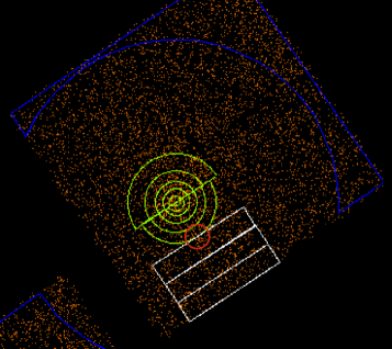
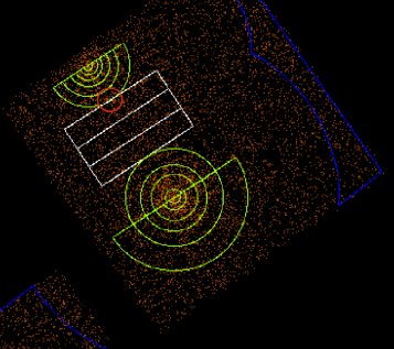
Figure 1.— Extraction regions for spectra in A1750. Observation IDs: 11878 and 11879 (upper and lower image). Green semi–annuli around the two cluster centers show the extraction regions for cluster emission, white rectangles show the regions we used for the interaction area. The red circles represent regions with substructure which we excised from our analysis. Regions excluded due to point source contamination are not shown to avoid clutter. The extraction regions for the background are represented with blue lines.

3. CHANDRA X–ray Data Analysis

In our X-ray analysis, we make use of two sets of observations of A1750 from the Chandra Data Archive (CDA) with ObsIDs: 11878 and 11879, and total exposure times of 19.77 ks and 20.05 ks respectively. We follow the standard data processing to reproduce event two files (evt2) from the event one files (evt1) using the latest Chandra Interactive Analysis of Observation (CIAO 4.4.1) with the updated Calibration Data Base (CALDB 4.5.1). Using the ev2 files, we detected and excluded the point sources using the CIAO script celldetect. Only a small fraction of the pixels were removed in the region we are interested in. The strong background flares, which are usually attributed to the high energy cosmic rays and would increase the event rates substantially higher, were cleaned by correcting the Good Time Interval (GTI) using the script lc_clean, excluding observation times for which the event rates were above or below 3$\sigma$. After all corrections had been applied, the total net exposure times were 11.515 ks and 12.481 ks for ObsIDs 11878 and 11879.

When analyzing targets with low X-ray surface brightness spacial care is needed to determine the background spectrum. Although most of the high energy particle background (e.g. cosmic rays) can be detected and filtered out during data processing, there is still some background contamination remaining. This background has two main components, the diffuse soft X-ray continuum background which dominates the energy below about 2–3 keV, and the higher energy cosmic rays randomly hitting the detectors. We excluded observations in time intervals in which they could be contaminated by cosmic rays using the standard method of running the script lc_clean with 3$\sigma$-clipping. The remaining X-ray background is customarily removed using background subtraction. The Chandra science team provides the blank-sky observations for the soft band background estimation, however, the blank-sky background observations were performed using the FAINT mode, while the two observations of A1750 the VFAINT mode was used. Also, the X-ray background shows fluctuations in different parts of the sky, therefore we choose to use local backgrounds. Thanks to the 16 ​$\arcmin$$\times$16 ​$\arcmin$ field of view of ACIS-I, A1750 fell only on two ACIS-I chips, we were able to extract spectra locally, from the other two ACIS-I chips and another front illuminated chip (ccd$\_$id = 7). This assures us that the background extraction regions are far enough from the peak emission ($\geq$ 11$\arcmin$) where the cluster emission is negligible. We also compared the resulting fitted temperature profiles of A1750 using local background spectra and the blank–sky spectra normalized in the 9.0–12.0 keV band, and found that they were consistent.

In order to study the temperature along the merging axis, we extracted two sets of semi–annuli centered on the peaks of A1750N and A1750C, [RA; DEC]=[13:31:10.94; $-1$:43:41.65] and [13:30:49.88; $-$1:51:46.7]. The merging axis goes through the middle of the semi–annuli as it is shown in Figure 1. We found a region with highly scattered temperature distribution (with temperatures above 12 keV) around the peak of A1750N at RA = 13:31:05.342, DEC = 01:45:45.78 due to a substructure (Okabe et al. 2011). We excluded this substructure from our analysis using a circular region with a radius of 45 ​$\arcsec$ around the peak of A1750N. We extracted spectra for the interacting region between the two peaks in three rectangles with length of 400 ​$\arcsec$ and width of 82.6 ​$\arcsec$ with their short symmetry axis aligned with the line of merging (see Figure 1).

We used the CIAO-4.4 software tool specextract to create the spectrum, the Response Matrix File (RMF) and the Ancillary Response File (ARF) for each region. The background spectra were extracted using the CIAO-4.4 software tool dmextract independently with the source spectra. We use the X-ray fitting package XSPEC-12.5 in our spectral analysis. The gas emission in each annulus is described by an optically thin plasma emission model, APEC, multiplied by the photo-electric absorption model, WABS. We fixed the galactic photoelectric column density absorption at 2.37$\times 10^{20}$ cm^-2 and the redshift at 0.086. We fitted the projected temperature, abundance and normalization parameters for each semi–annulus in the energy band 0.5–7.0 keV using C-statistic.

Figure 2.— Projected temperature in A1750 from Chandra observations (points with error bars). The gray vertical dashed lines show the centers of the two components A1750N and A1750C.

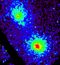
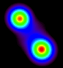
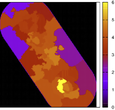
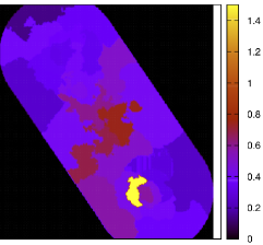
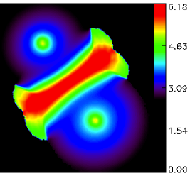
Figure 3.— Images of X–ray surface brightness and projected temperature (in units of keV) of A1750 from Chandra observations and from our FLASH simulation with an impact velocity of 1400 $\rm km\;s^{-1}$ (run: R3V14P15), which is the best match to X–ray, optical and infrared observations. From left to right: 1st row: exposure corrected X–ray surface brightness map from observations, surface brightness map from simulation; 2nd row: projected temperature and error map from observations and our simulation.

In Figure 2 we show our results on the projected X–ray temperature as a function of distance defined along the line connecting the two X–ray peaks (the centers of the two main components), setting the origin at the center of A1750N. The data points (squares) with error bars represent the results from a simultaneous fit to both Chandra observations (ObsIDs 11878 and 11879). Fits to individual observations are consistent with the simultaneous fit, although ObsID 11879 show larger dispersion. Our results from the simultaneous fitting are in good agreement with those based on XMM-Newton observations (Belsole et al., 2004).

We find that the projected model temperature keeps increasing towards the center of A1750C (in agreement with Belsole et al.) implying that is not a cool core cluster, since the projected temperature keeps increasing towards the center, unlike A1750N, which has a decreasing temperature profile towards its center (see Figure 2). The temperatures at about 0.2 Mpc from the centers of the two components located at 0.2 and 0.7 Mpc, are about 3.5 and 4 keV respectively, increasing toward the middle of the interaction region (0.3–0.6 Mpc) to about 6 keV. This is a clear sign of a compressed, shock heated intracluster gas between the two merging clusters. This high temperature region is clearly not in hydrostatic equilibrium in the gravitational potential of A1750.

Table 1Initial Parameters and rotation angles

ID	V[km s${}^{-1}]$	P[kpc]	$\theta[^{\circ}]\;\;\;\;\;$
R1V05P15	500	150	16.9$\pm$2.6
R2V08P15	800	150	21.1$\pm$3.2
R3V14P15	1400	150	28.2$\pm$4.3
R4V16P15	1600	150	30.2$\pm$4.8
R5V35P15	3500	150	46.0$\pm$7.2
R6V08p00	800	0	21.2$\pm$3.4
R7V08p20	800	200	24.6$\pm$3.9

4. FLASH Simulations

We carried out three–dimensional self-consistent numerical simulations of binary galaxy cluster mergers including dark matter and intracluster gas using the publicly available parallel Eulerian parallel code, FLASH, developed at the Center for Astrophysical Thermonuclear Flashes at the University of Chicago (for a detailed description see Fryxell et al. 2000 and Ricker 2008). The highest resolution (cell size) of 12.7 kpc we reached at the cluster centers and in the regions of merger shocks. Our box size was 13.3 Mpc on a side. Our simulations were semi–adiabatic in the sense that only adiabatic processes and shock heating were included (no other non–gravitational effects). A detailed description of the set up for our simulations can be found in Molnar et al. (2012). We briefly summarize the main points here.

4.1. Initial Conditions

Spherical symmetry is assumed for each of the two interacting clusters for both the gas and the dark matter within the the virial radius of each cluster. We used a truncated NFW model (Navarro, Frenk & White, 1997) for the dark matter distribution:

$$\rho_{DM}(r)={\rho_{s}\over x(1+x)^{2}},$$ (1)

where $\rho_{s}$ is the scaling parameter for the density, $x=r/r_{s}$, where $r_{s}=R_{vir}/c_{vir}$ is the scaling parameter for the radius, and $c_{vir}$ is the concentration parameter. We assume a truncated non-isothermal $\beta$ model for the gas:

$$\rho(r)={\rho_{0}\over(1+y^{2})^{3\beta/2}},$$ (2)

where $y=r/r_{core}$, and $\rho_{0}$, $r_{core}$ are the central density and gas scale radius, and $r\leq R_{\rm vir}$. The temperature of the gas was determined form the equation of hydrostatic equilibrium via numerical integration to ensure an initial equilibrium configuration for each of the two main mass components. The equation of state for the gas was an ideal gas equation of state with $\gamma=5/3$. We adopted $r_{core}=0.08$ $R_{\rm vir}$, and, since we are interested in the outer parts of the intracluster gas, $\beta=1$ (which is suggested by cosmological numerical simulations, Molnar et al. 2010a).

We adjust the initial concentrations of the dark matter components in order to approximately reproduce the gas temperature profile lying well away from the gas interaction zone, as described in the next subsection. Our dark matter particles also represent stellar matter in galaxies as this component may also be considered collisionless. The number of dark matter particles at each AMR cell was determined by the local density, with the total number of 5 million dark matter particles used in our simulations. In our simulations, we assume a gas mass fraction of 0.14 initially.

The velocities of the dark matter particles were determined by sampling a Maxwellian distribution with the velocity dispersion, $\sigma_{r}$, derived from the Jeans equation (Łokas & Mamon, 2001). Assuming isotropic velocity dispersion (the angular and radial components are equal: $\sigma_{\theta}=\sigma_{r}$), and NFW models, we obtain

$$\sigma_{r}^{2}(r)=V_{v}^{2}\,g(c_{vir})\,x\,q^{2}\int_{x}^{\infty}\Biggl{[}{\ln q\over x^{3}q^{2}}-{c_{vir}\over x^{2}q^{3}}\Biggr{]}dx,$$ (3)

where $q=1+x\,c_{vir}$, the circular velocity is $V_{v}^{2}=GM_{vir}/R_{vir}$, and

$$g(c_{vir})=\bigl{[}\ln(1+c_{vir})-c_{vir}/(1+c_{vir})\bigr{]}^{-1}.$$ (4)

The direction of the velocities were assumed to be isotropic (for a more detailed description see Molnar et al. 2012).

Figure 4.— Projected X–ray temperature in A1750 from Chandra observations (points with error bars) and from FLASH simulations (runs: R1V05P15, R3V14P15 and R5V35P15) from radial half circle regions around the two main clusters and rectangle regions between them (regions shown in Figure 1). We sample a range of impact velocities of 500, 1400, and 3500 $\rm km\;s^{-1}$ (continuous, dash–dotted, and dashed lines). The region between the vertical dashed lines represent the extraction region for the spectra for the interaction region (region 3 in Figure 1).

4.2. FLASH Runs of Merging Clusters

We performed simulations to find the best model for A1750, and, in general, to identify initial parameters we can determine for a merging cluster before the first core passage. Our main focus is on determining the impact velocity of the merger, because of its relevance for cosmology.

We use gravitational lensing measurements as our starting point. These lensing measurements are very important when using numerical simulations to interpret observations of merging galaxy clusters because they can be used to identify and constrain the main mass components of the system. In particular, the morphology of the reconstructed mass surface distribution tells us about how many components are in the system, and the projected positions of the components give us information about the phase of the collision (i.e., the time before or after first core passage). Perhaps even more importantly, we can get mass estimates for the components, which can reduce the initial parameter space substantially we need to search when we run a set of simulations.

Firstly we run a series of simulations of galaxy cluster mergers with different concentration parameters and with the masses of each of the two main components covering 1–5 $\times 10^{\,14}\,$$\mbox{\rm M}_{\odot}$. This is chosen to be roughly within the range allowed by the lensing analysis of Okabe & Umetsu (2008), except that we did not consider masses larger than 5 $\times 10^{\,14}\,$$\mbox{\rm M}_{\odot}$ because their virial radii would be too large and therefore the temperature increase in the interaction region would be much greater than what observed (no useful constraints on concentration parameters are available from lensing). We find that assuming total masses, $M\,^{C}=2.0$ and $M\,^{N}=1.8$ $\times 10^{\,14}\,$$\mbox{\rm M}_{\odot}$ and concentration parameters of 8 and 10 for the the main and the infalling cluster, we can reproduce the projected temperature profiles of the central regions of both clusters in the undisturbed cluster regions, away from the gas interaction zone in between the clusters.

Figure 5.— Same as Figure 4, but from our FLASH simulations with different impact parameters of 0, 150, and 200 kpc (dashed, continuous, and dash–dotted lines; runs: R6V08p00, R2V08P15, and R7V08p20).

In the next step, we hold the two masses and concentration parameters fixed at these values, and run a set of simulations systematically changing the impact parameters and relative velocities. In Table 1 we summarize the initial parameters for those runs we discuss in detail in our paper. In this table the first column is the identification number for our runs using the following convention: the numbers after V and P represent the initial relative velocity in units of 100 $\rm km\;s^{-1}$, and the impact parameter in units of 10 kpc. In the second and third columns we list the initial velocities and impact parameters, the third column shows the angle, $\theta$, we rotated the system out of the plane of the sky towards the observer (along an axis which is perpendicular to the line connecting the two cluster centers) in order to reproduce the observed projected distance between the two X–ray peaks.

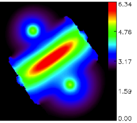
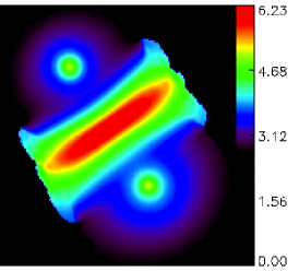
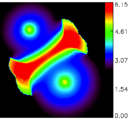
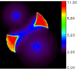
Figure 6.— Projected X–ray temperature maps from our FLASH simulations in units of keV, which provide a good match to the observed projected temperature distribution in A1750 (see Figure 4). From left to right: temperature maps from simulations with initial velocities of 500 and 800 $\rm km\;s^{-1}$ (runs: R1V05P15 and R2V08P15, 1st row), and with 1400, 1600, and 3500 $\rm km\;s^{-1}$ (runs: R3V14P15, R4V16P15, and R5V35P15, 2nd row). The interaction regions with an enhanced temperature of about 6 keV (red color) can be clearly seen in these images between the peaks corresponding to the two subclusters (except in the last one, where the maximum temperature is 10–11 keV).

4.3. Simulated Images

After each simulated collision is completed, we generate X–ray surface brightness and projected X–ray temperature images for a range of viewing angles. We align the two mass centers with the $x$ coordinate axis choosing the $y$ axis so that the $x-y$ plane coincides with the plane of the collision, which we first consider to be the plane of the sky. Then, we rotate our cluster around the $x$ axis with a roll angle, $\phi$, (active rotation), then around the $y$ axis by a polar angle of $\theta$. Therefore, with this definition, zero rotation angles ($\phi=0$, $\theta=0$) mean that the collision is in the plane of the sky. Once we choose the roll angle and the polar angle, we generate the X–ray surface brightness image by performing a line–of–sight (LOS) integral

$$I_{X}(x,y)\propto\int_{\ell_{1}}^{\ell_{2}}\rho_{g}^{2}\,\Lambda(Z_{ab},T_{g})\;d\ell,$$ (5)

where $\ell$ is the spatial coordinate in the LOS, and we used the publicly available APEC code for the frequency integrated cooling function, $\Lambda$, since in the early phase of the merging (well before first core passage), the temperature does not get above about 12 keV, therefore we do not need relativistic corrections. We convolve the derived total spectrum in each pixel of the resulting map with a piecewise linear approximation of the on–axis affective area of the ACIS–I CCD, to derive the final simulated image of the X–ray surface brightness.

We approximate the observed projected X–ray temperature for our merging clusters using the spectroscopic-like X-ray temperature proposed by Mazzotta et al. (2002), which is a weighted average of the physical temperature in the LOS,

$$T(x,y)\approx T_{sp}(x,y)={\int w_{sp}\;T_{g}\;d\ell\over\int w_{sp}\;d\ell},$$ (6)

where the weight is $w_{sp}=\rho^{2}/T_{g}^{3/4}$. This projected temperature has been shown to be a good approximation to cluster temperature profiles similar to those observed with Chandra and XMM-Newton (Nagai, Kravtsov & Vikhlinin, 2007).

5. Results and Discussion

Our results for the simulated projected temperature distributions for different impact velocities as well as different impact parameters are shown in Figures 4 and 5. In Figure 4 we show projected X–ray temperatures from simulations with impact velocities of 500, 1400, and 3500 $\rm km\;s^{-1}$ (continuous, dash–dotted, and dashed lines). The region between the two vertical dashed lines represents the interaction region. The rotation angle out of the plane of the sky, $\theta$, and the phase of the collision (the time before first core passage) are set such that the projected distance is equal to the observed separation of 900 kpc, and the projected temperature profile simultaneously matches the profile we derived from X–ray observations (see Table 1). Note that we did not aim to model the cool core of A1750N since we are interested in the interaction region, thus we do not expect to reproduce the projected temperature in the core.

We focus on modeling the interaction region, which is between the two temperature peaks excluding the core regions around the clusters within a radius of about 0.2 kpc, which is, in our distance coordinate, from 0.15 to 0.8 Mpc. We obtain acceptable fits in the interaction region to all impact velocities we considered, except the high impact velocity of 3500 $\rm km\;s^{-1}$, for which the simulated temperature profile deviates more than 2$\sigma$ from all three data points in this region (three points in the middle). Based on this figure, we conclude that a large impact velocity for A1750 is very unlikely.

We show the effect of different impact parameters in Figure 5. It can be seen from this figure that varying the impact parameter over 0, 150, 200 kpc does not change the projected temperature significantly. Clearly, the projected temperature is not sensitive to a moderate change in the impact parameter, therefore we can not put meaningful constraint on this parameter. Therefore we use our results for runs with fixed impact parameter at 150 kpc in the following discussion.

As a next step, we check if we can use the morphology of the projected X–ray temperature to further constrain the impact velocity of A1750. We show images of the exposure corrected X–ray surface brightness and projected temperature based on the merged Chandra observations of A1750 with ObsIDs 11878 and 1187 in Figure 3. The enhancement between the two main clusters can be clearly seen in the surface brightness image (1st row 1st panel). In the 2nd row 1st and 2nd panels we show the images of the projected temperature and the corresponding error using adaptive binning of the image based on surface brightness contours following the method described by Sanders (2006). The errors in the temperature in the interaction region are large, about 1 keV, due to the low surface brightness and the short exposure time. The surface brightness contours in this region are dominated by noise, therefore the temperature map is not reliable (the projected temperature map in the interaction region based on the merged observations do not agree with those from on the individual observations). We can only conclude that there seem to be no large temperature peaks or troughs in this region. Our surface brightness and projected temperature temperature maps are consistent with those of Belsole et al. (2004), who used a 34 ks XMM-Newton observation of A1750 (their Figure 2 and 5). The projected temperature map of A1750 from XMM-Newton observations has an error of about 0.6 keV in the interaction region showing a temperature enhancement with no significant increase or decrease towards the middle of the region.

The images of the projected temperature from our FLASH simulations with impact velocities of 500, 800, 1400, 1600, and 3500 $\rm km\;s^{-1}$ (runs R1V05P15, R2V08P15, R3V14P15, R4V16P15, and R5V35P15; left to right, 1st and 2nd row) are shown in Figure 6. The rotation angles and phases of collision are different for these runs chosen to match the observed projected distance and temperature profile of A1750 (see Table 1 and Figure 4). The two peaks on the lower right and upper left corner in each image mark the cluster centers. The enhanced projected temperature region in the middle is the interaction region. Since we need larger rotation angles out of the plane of the sky for larger velocities in order to have more cooler gas in the LOS to lower the projected temperature to match with the observations, the different morphology is due to the different rotation angles. Therefore, as we can see it from Figure 6, in general, the temperature distribution in the interaction region has a bump in the middle for low impact velocities and turns into a saddle shape for larger velocities as a function of the rotation angle, $\theta$.

Our simulations assuming an impact velocity of 1400 $\rm km\;s^{-1}$ and 1600 $\rm km\;s^{-1}$ (runs R3V14P15 and R3V16P15) with a flat plateau of about 6 keV in the projected temperature in the interaction region (1st and 2nd panel in the 2nd row in Figure 6) have the most similar morphology to those from our Chandra analysis (2nd row 1st panel in Figure 3) and from the XMM-Newton observation of A1750 (Figure 5 of Belsole et al. 2004). There are some small deviations due to substructure we have not modeled in our simulations, but the interaction region looks very similar. In this region R3V14P15 and R3V16P15 show different morphology at the level of about 0.5 keV, but these systematic variations are not significant, they are in the same order as the errors from observations. Therefore, unfortunately, we can not derive an accurate impact velocity for A1750 based on the available projected temperature maps, because neither the Chandra nor the XMM-Newton observations have sufficient exposure time to construct an accurate projected temperature map. However, in principle, the morphology of the projected temperature can be used to put strict constraints on the impact velocity for merging clusters. Our results from simulations suggest that if we have observed projected temperature maps with errors less than 0.5 keV, we may be able to constrain the impact velocities of merging clusters to 200–300 $\rm km\;s^{-1}$ (compare 1st to 2nd panels in the 1st as well as in the 2nd row in Figure 6).

The Mach number for our best fit model (run R3V14P15, see Figure 3) can be calculated from our simulations directly. We show the physical temperature and pressure profiles of the gas along a line crossing the shocks as a function of distance (same spatial coordinate as in Figure 4) in units of keV and, 4$\times 10^{11}$ dyne cm^-2, to be able to see their features in the same plot for easy comparison. The temperature peak of about 11 keV in the middle of the interaction region is due to previous shock activity followed by adiabatic compression at the contact discontinuity (no jump in the pressure here). The temperature and pressure jumps at -170 kpc and 180 kpc belong to the two shock fronts we can see before the first core passage. We calculate the Mach number from the usual Rankine–Hugoniot jump conditions using the pressure jump:

$${\cal M}=\Biggl{[}0.8\,\frac{P_{2}}{P_{1}}+0.2\Biggr{]}^{1/2},$$ (7)

where $P_{1}$ and $P_{2}$ are the upstream (pre-shock) and downstream (post-shock) pressures at the position of the shock, and we assumed $\gamma=5/3$, as in Molnar et al. (2009), where the advantages of using the pressure is discussed. Since the pressure jumps are similar in both shocks, we get similar Mach numbers, 1.4 and 1.2, for the shock front on the left and the right.

Figure 7.— Projected temperature change as a function of rotation angle ($\theta$, in Degrees) at the center of the contact discontinuity for R3V14P15 (the same run and phase as in Figure 3). In this Figure we show the temperature change along the line connecting the two cluster centers marked by the peaks in the projected X–ray temperature maps (see Figure 6).

Belsole et al. (2004) estimated the Mach number for the shock assuming that the gas is close to isothermal and in equipartition after the shock, suggested by Markevitch et al. (1999), in which case the Rankine–Hugoniot jump conditions imply that

$${\cal M}=\sqrt{3{\cal C}\over 4-{\cal C}},$$ (8)

where the shock compression, ${\cal C}$, can be derived from

$${1\over{\cal C}}=\Biggl{[}4\biggl{(}{T_{2}\over T_{1}}-1\biggr{)}^{2}+{T_{2}\over T_{1}}\Biggr{]}^{1/2}-2\biggl{(}{T_{2}\over T_{1}}-1\biggr{)},$$ (9)

assuming $\gamma=5/3$. Belsole et al. obtained a Mach number of 1.64 assuming pre shock temperature of $T_{1}=3.1$ and for the post shock temperature, the global temperature of the interaction region, $T_{2}=5.1$. As we can see this estimated Mach number is in a good agreement with that we derived from our simulations directly, but this is only a coincidence since some of the temperature increase in the interaction region comes from adiabatic compression and not from a shock. From Figure 8 we can see that a global temperature in the interaction region would be about 8 keV not 5.1 keV as measured by Belsole et al. (2004) from XMM-Newton data, and would result in an overestimate of the Mach number (2.4), but, as we pointed out, the projected temperature is, in general, and in this region, an underestimate of the physical temperature due to cool gas in the LOS. We illustrate this point in Figure 7). In this figure, we show how the projected peak temperature changes as a function of rotation angle out of the sky ($\theta$) using the same run (R3V14P15) and phase as we used in Figure 3. We find that the peak temperature on the line connecting the two cluster centers (in this simulation) decreases substantially with angle from about 6 keV at $\theta=0$, to zero keV at about $\theta$ = 60$\!\!{}^{\circ}$.

Figure 8.— Physical temperature and pressure (solid and dashed line) across the shock as a function of distance for run R3V14P15 (the same run and phase as in Figure 3). The distance coordinate is the same as in Figure 4). The shock can be clearly seen on the two sides of the interaction region: as a temperature and pressure jump. The maximum temperature is at the contact discontinuity, where there is no pressure jump.

As a last step, we investigate wether we can use galaxy redshift measurements in the field of A1750 to quantify the impact velocity in this merging cluster. We collected galaxy redshift measurements in the vicinity of A1750 from NED. We found 195 galaxies within 30 ​$\arcmin$ from the center of A1750 with redshifts between 23000 $\rm km\;s^{-1}$ and 28000 $\rm km\;s^{-1}$. We show the positions of galaxies in the field of A1750 in Figure 9. Squares mark the centers of the two subclusters. We show the number distribution of the velocities of these galaxies in Figure 10. The histogram with a dash–dotted line represents all galaxies, histograms with dashed and continuous lines show distributions of galaxy velocities within a radius of half of the distance between centers of A1750C and A1750N (about 1R₅₀₀). We find radial velocities of 25999$\pm 80$ $\rm km\;s^{-1}$ and 25034$\pm 101$ $\rm km\;s^{-1}$for A1750C and A1750N respectively. We can conclude that A1750C is closer to us moving towards A1750N, which is farther from us. This is why the A1750C, which is closer to us, has a larger redshift. As we can see, redshift measurements can break the degeneracy of the spatial distribution in the LOS inherent in our X–ray and gravitational lensing observations. To derive the projected instantaneous relative velocity from these redshift measurements we fitted gaussians to the peaks of the observed velocity distributions of the two components to derive their relative LOS velocities. The results are shown in Figure 10 (solid and dashed Gaussians). The positions of the two peaks of the Gaussian fits agree with the two local maxima of the histogram representing the total galaxy distribution, as we would expect. We obtained a LOS velocity of $V_{r}=960\pm$130 $\rm km\;s^{-1}$. This should be considered to be a lower limit for the impact velocity for A1750 because of the significant projection angle implied by the X–ray analysis above, and because the relative velocity increases until the first core passage.

Using the fewer galaxy redshifts available at that time and adopting a biweight analysis applicable to low-number statistics, as suggested by Beers et al. (1990), Hwang & Lee (2009) found radial velocities of 25931${}_{-201}^{+212}$ $\rm km\;s^{-1}$ and 24999${}_{-172}^{+260}$ $\rm km\;s^{-1}$ for A1750C and A1750N, and thus obtained $V_{r}=932\pm 332$ $\rm km\;s^{-1}$ (Table 2 in Hwang & Lee). The differences in the radial velocities of the two components and their relative velocities between our results and those of Hwang & Lee are only 68, 35 and 28 $\rm km\;s^{-1}$, each is only a small fraction of the 1$\sigma$ errors, thus we conclude that our results are in good agreement with those of Hwang & Lee.

Comparing the instantaneous radial velocities of our simulations determined from the rotation angles derived from the projected temperature profiles (last column in Table 1), we derive the initial relative velocity of 1460${}_{-200}^{+180}$ $\rm km\;s^{-1}$ (uncertainties in the rotation angle and radial velocity contributing about 130–150 $\rm km\;s^{-1}$ each). In Figure 3 (1st row 2nd panel and 2nd row 3rd panel), we show the images of the X–ray surface brightness and projected temperature from our FLASH simulation with an impact velocity of 1400 $\rm km\;s^{-1}$ (run: R3V14P15) which is the best match to X–ray, optical and infrared observations of A1750. The enhancement in the surface brightness within the two X–ray peaks marking the centers of the merging clusters can be clearly seen in the simulated image (1st row 2nd panel), and similarly to the Chandra surface brightness image (1st row 1st panel). In the image of the projected X–ray temperature from our simulations (2nd row 3rd panel), the maximum temperature (red) in the middle of the interaction region is about 6 keV, which is consistent with our temperature map from the Chandra observations (2nd row 1st panel) within errors. Based on this figure, we conclude that the morphology of the simulated images of the X–ray emission and the projected temperature are in good agreement with those from our Chandra analysis (1st row 1st panel and 2nd row 1st panel) and those based on XMM-Newton observations of A1750 (images in Figure 5 of Belsole et al. 2004).

Figure 9.— The distribution of galaxies in the field of A1750. The coordinates are relative positions to the center of the image in units of Degrees (plus signs). The centers of the A1750C (close to the center) and A1750N (to the North) are marked with squares. The circles show the extraction regions we used in our histograms of velocity distributions (see Figure 10). The radii of the circles are equal to the half distance between the centers of the subclusters (about R₅₀₀).

We compare our results for the velocity and rotation angle from simulations to those obtained applying the two-body dynamical model introduced by Beers et al. (1982). This simplified model for binary galaxy cluster mergers assumes that the two components start out at time zero with zero spatial separation on a radial orbit ignoring a likely finite angular momentum of the system and any tidal forces due to the large scale structure. Since the X–ray observations suggest that the two subclusters are moving towards each other, we are looking for a bound solution. In this case the system can be described by the well known parametric solution of Einstein’s field equations:

$$R_{3D} = \frac{R_{max}}{2}\bigl{(}1-\cos\chi\bigr{)}$$ (10)

$$V_{3D} = \Biggl{[}\frac{2GM}{R_{max}}\Biggr{]}^{1/2}\frac{\sin\chi}{1-\cos\chi}$$ (11)

$$t = \Biggl{[}\frac{R_{max}^{\,3}}{8GM}\Biggr{]}^{1/2}\bigl{(}\chi-\sin\chi\bigr{)},$$ (12)

where $R_{3D}$ and $V_{3D}$ are the 3D distance and relative velocity between the two components, $t$ is the time elapsed since zero separation, $R=0$, which we assume to be equal to the age of the Universe at the redshift of A1750, $t=t_{z}=12.34$ Gyr in our concordance $\Lambda$CDM, $R_{max}$ is the distance at maximum separation, $M=M_{C}+M_{N}=3.8$ $\times 10^{\,14}\,$$\mbox{\rm M}_{\odot}$ is the total mass of the system, $G$ is the gravitational constant, and $\chi$ is the development angle.

Figure 10.— Velocity distribution of galaxies in the vicinity of A1750. The dash–dotted histogram represents all galaxies in the field (see Figure 9). Histograms with solid and dashed lines show distributions of velocities of galaxies within circles around A1750N and A1750C (see Figure 9). Gaussian fits to the histograms of the two subclusters are shown with the same line codes.

The rotation angle between the line of collision and the plane of the sky, $\theta$, connects the observables, the projected distance, $R_{p}$, and relative radial velocity, $V_{r}$, to these equations: $R_{p}=R\cos\theta$ and $V_{r}=V\cos\theta$. Based on our results, we adopt $R_{p}=900$ kpc and $V_{r}=960\pm 129$ $\rm km\;s^{-1}$. We ignore the error in $R_{p}$ since is much less than that in $V_{r}$. Following Gregory & Thompson (1984), we substitute the observables into Equations 10, 11, and 12, and derive a relation between the rotation angle, $\theta$ and the development angle:

$$\tan\theta=\frac{t_{z}\,V_{r}}{R_{p}}\frac{(\cos\chi-1)^{\,2}}{\sin\chi\,(\,\chi-\sin\chi\,)}.$$ (13)

Using Equations 10–13, we obtain $V_{3D}$ = 1171${}_{-259}^{+231}$ $\rm km\;s^{-1}$ and $\theta$ = 52.$\!\!{}^{\circ}$9${}_{\;+14.^{\!\!\!\circ}7}^{\;-9.^{\!\!\!\circ}10}$ (errors in the angle run from +14.7 to -9.10 because the higher the velocity the lower the rotation angle). The instantaneous relative 3D velocity we obtain from our best fit model is 1992 $\rm km\;s^{-1}$ (with a rotation angle of $\theta$ = 28.$\!\!{}^{\circ}$8) is significantly higher than the predictions of the dynamical model signaling a possible tension between observations and $\Lambda$CDM predictions for relative velocities of massive clusters. However, this comparison is not conclusive because the assumptions of our dynamical model are not satisfied. Including the mass of the component farther to the South of A1750C and A1750N in the total mass of the system does not increase the predicted relative velocity of the dynamical model significantly since its mass is much less than 10% of $M_{1}+M_{2}$ (Hwang & Lee, 2009), and thus does not change our conclusion. Note that the predictions for the impact velocity from our simulations are not affected by the less massive component to the South because we start our simulations at the time of impact, and from that point of time the gravitational field is dominated by the two components we are following.

Summarizing our results: we found that our FLASH simulations can reproduce the X-ray morphology, projected temperature distribution and galaxy redshift measurements of A1750 assuming that the relative impact velocity is V = 1460${}_{-200}^{+180}$ $\rm km\;s^{-1}$ and the rotation angle from the plane of the sky is $\theta$ = 28.$\!\!{}^{\circ}$8$\pm$4.$\!\!{}^{\circ}$4. This velocity is higher than the average impact velocity for this mass range, 600 $\rm km\;s^{-1}$, predicted by the concordance $\Lambda$CDM model, but it is within the allowed range. Our results suggest that we can eliminate the possibility of a large impact velocity greater than 2000 $\rm km\;s^{-1}$ (at 99.7% CL) for this merging cluster since that would imply a much larger relative radial velocity than the observed. Note that the quoted uncertainties refer to statistical errors due to observations based on our idealized cluster merging simulations. These errors do not reflect possible systematic errors due to asphericity, substructure (visible in the XMM-Newton image of the system; see Figure 2 of Belsole et al. 2004), gas falling in along the filament between the two components, and deviations due to the lack of hydrostatic equilibrium at the outer regions of clusters (e.g., Sereno et al. 2013; Ichikawa et al. 2013; Chiu & Molnar 2012; Laganá et al. 2010; Molnar et al. 2010b; and references therein), and modeling uncertainties in the outer regions of clusters due to weak constraints from observations, which have not been quantified in this context. Although the systematic effects might be larger than our statistical errors, we do not expect large changes (say a factor of two) in the derived impact velocity for A1750 from systematic effects because the intracluster gas of each component is compressed over a wide radial range, from $\sim$300 kpc to $\sim$1000 kpc into a 200 kpc region from $\sim$300 kpc (the inner limit of the interaction region) to $\sim$500 kpc (the position of the contact discontinuity, see Figure 8). Therefore the resulting density and temperature profiles, for comparison with the data, should not be very sensitive to the initial conditions of the gas.

6. Conclusion

We have been carrying out self–consistent N/body–hydro-dynamical simulations (including dark matter and gas) to investigate how we can best determine the impact velocities of merging galaxy clusters. We have demonstrated, that the impact velocities can be determined in an early stage of merging, in the case of A1750, well before the first core passage with the use of multi–wavelength data and hydrodynamical simulations. The physical basis which enables us to derive the impact velocity of a merging system before the first core passage is that the temperature of the shocked gas depends on the relative velocities of the two subclusters.

Observations do not provide the physical temperature of the gas in clusters directly, but only the projected temperature, which can be substantially lower than the physical temperature due to the averaging along the line of sight in projection which could contain a substantial amount of cold gas. We have shown with our models that the observed (projected) temperature depends on the angle we rotate the system towards the observer around the axis perpendicular to the line connecting the centers of the two subclusters. Even without rotation, the projected temperature is about 1–2 keV lower than the physical temperature. We demonstrated that this degeneracy can be resolved using the morphology of the merging system and independently using the observed galaxy redshift information, and thus a more accurate determination of the impact velocity is possible. As a consequence, we conclude that the conventional method deriving the impact velocities for merging systems is not reliable due to two erroneous assumptions: (1) the measured projected temperature is the physical temperature; (2) the temperature of the interaction region is exclusively coming from the shock.

As a case study, we used multi–wavelength observations and numerical simulations to constrain the impact velocity in the merging galaxy cluster A1750. Results from previous weak lensing analysis were used here to constrain the masses of the two main components, and member galaxy redshifts constrained the projected LOS instantaneous relative velocities of the two merging clusters. We used X–ray measurements to constrain the impact velocity and rotation angle of the plane of the collision relative to the LOS. We found that among our idealized cluster merging simulations with the input masses constrained to be $M\,^{C}=2.0$ and $M\,^{N}=1.8$ $\times 10^{\,14}\,$$\mbox{\rm M}_{\odot}$, the concentration parameters fixed at 8 and 10, and impact parameter at 150 kpc, the simulation with a relative velocity of 1460 $\rm km\;s^{-1}$ matches all available observations well. Impact velocities in excess of 2000 $\rm km\;s^{-1}$ are unlikely because, either the implied instantaneous relative velocities would exceed the observed LOS relative velocity of 900 $\rm km\;s^{-1}$, or the collision would have to lie very close to the plane of the sky, in which case a high velocity impact is excluded by the high projected X–ray temperature in the interacting region which is measured to be only about 6 keV by the X–ray observations. Our constraints on the infall velocity are stronger from the radial velocity difference derived from optical observations because we do not have strong constraint from the gas morphology from the relatively short X–ray exposures.

Impact velocities of merging systems soon after the first core passage have been derived from multi-wavelength observations and numerical simulations for two clusters (the bullet cluster: Springel & Farrar 2007; Mastropietro & Burkert 2008, and references therein, and CL0152-1357: Molnar et al. 2012). The resulting infall velocities were very high, from 3000 $\rm km\;s^{-1}$ to 4800 $\rm km\;s^{-1}$, illustrating the considerable differences between these velocities and infall velocities inferred by the $\Lambda$CDM model. The advantage of focusing on deriving impact velocities of merging clusters before the first core passage is that merging essentially begins in this phase and are not yet significantly speeded up, deflected and suffering considerable ram pressure which is sensitive to the impact parameter. Several well observed examples of pre–merger clusters would allow this approach to be applied to existing lensing and X–ray data (see Maurogordato et al. 2011; Okabe & Umetsu 2008, and references therein). The importance of a clear understanding of the relative impact velocities is highlighted by the anomalously high velocities inferred for such systems and the difficulty of reproducing these velocities within the conventional $\Lambda$CDM framework. Any significant asymmetry in the distribution of pre–merger and post–merger relative velocities would be of great interest for alternative models of gravity and for the BEC model of dark matter where coherent non–linear wavelike behavior of the dark matter (González & Guzmán, 2011) may generate unexpected behavior during interactions.

References

- Beers et al. (1982) Beers, T. C., Geller, M. J., & Huchra, J. P. 1982, ApJ, 257, 23
- Beers et al. (1990) Beers, T. C., Flynn, K., & Gebhardt, K. 1990, AJ, 100, 32
- Belsole et al. (2004) Belsole, E., Pratt, G. W., Sauvageot, J.-L., & Bourdin, H. 2004, A&A, 415, 821
- Bradač et al. (2006) Bradač M., Clowe D., Gonzalez A. H., Marshall P., Forman W., Jones C., Markevitch M., Randall S., et al., 2006, ApJ, 652, 937
- Chiu & Molnar (2013) Chiu & Molnar 2013, ApJ, 222, 222
- Chiu & Molnar (2012) Chiu, I.-N. T., & Molnar, S. M. 2012, ApJ, 756, 1
- Clowe et al. (2006) Clowe D., Bradač M., Gonzalez A. H., Markevitch M., Randall S. W., Jones C., & Zaritsky D., 2006, ApJ, 648, L109
- Clowe et al. (2004) Clowe D., Gonzalez A., & Markevitch M., 2004, ApJ, 604, 596
- Donnelly et al. (2001) Donnelly, R. H., Forman, W., Jones, C., et al. 2001, ApJ, 562, 254
- Forman et al. (1981) Forman, W., Bechtold, J., Blair, W., et al. 1981, ApJ, 243, L133
- Fryxell et al. (2000) Fryxell, B., et al. 2000, ApJS, 131, 273
- González & Guzmán (2011) González, J. A., & Guzmán, F. S. 2011, Phys. Rev. D, 83, 103513
- Gregory & Thompson (1984) Gregory, S. A., & Thompson, L. A. 1984, ApJ, 286, 422
- Harko (2011a) Harko, T. 2011a, Phys. Rev. D, 83, 123515
- Harko (2011b) Harko, T. 2011b, MNRAS, 413, 3095
- Hayashi & White (2006) Hayashi E., White S. D. M., 2006, MNRAS, 370, L38
- Hwang & Lee (2009) Hwang, H. S., & Lee, M. G. 2009, MNRAS, 397, 2111
- Ichikawa et al. (2013) Ichikawa, K., Matsushita, K., Okabe, N., et al. 2013, ApJ, 766, 90
- Kain & Ling (2012) Kain, B., & Ling, H. Y. 2012, Phys. Rev. D, 85, 023527
- Lee & Komatsu (2010) Lee J., Komatsu E., 2010, ApJ, 718, 60
- Korngut et al. (2011) Korngut, P. M., Dicker, S. R., Reese, E. D., et al. 2011, ApJ, 734, 10
- Laganá et al. (2010) Laganá, T. F., de Souza, R. S., & Keller, G. R. 2010, A&A, 510, A76
- Łokas & Mamon (2001) Łokas, E. L., & Mamon, G. A. 2001, MNRAS, 321, 155
- Madarassy & Toth (2002) Madarassy, E. J. M., & Toth, V. T., 2012, arXiv:1207.5249
- Markevitch et al. (1999) Markevitch, M., Sarazin, C. L., & Vikhlinin, A. 1999, ApJ, 521, 526
- Markevitch et al. (2004) Markevitch, M., Gonzalez, A. H., Clowe, D., et al. 2004, ApJ, 606, 819
- Massardi et al. (2010) Massardi, M., Ekers, R. D., Ellis, S. C., & Maughan, B. 2010, ApJ, 718, L23
- Mastropietro & Burkert (2008) Mastropietro, C., & Burkert, A. 2008, MNRAS, 389, 967
- Maurogordato et al. (2011) Maurogordato, S., Sauvageot, J. L., Bourdin, H., et al. 2011, A&A, 525, A79
- Mazzotta et al. (2002) Mazzotta P., Rasia E., Moscardini L., & Tormen G., 2004, MNRAS, 354, 10
- Molnar et al. (2012) Molnar, S. M., Hearn, N. C., & Stadel, J. G. 2012, ApJ, 748, 45
- Molnar et al. (2010a) Molnar, S. M., et al. 2010a, ApJ, 723, 1272
- Molnar et al. (2010b) Molnar, S. M., Chiu, I.-N., Umetsu, K., et al. 2010b, ApJ, 724, L1
- Molnar et al. (2009) Molnar, S. M., Hearn, N., Haiman, Z., et al. 2009, ApJ, 696, 1640
- Mroczkowski et al. (2012) Mroczkowski, T., et al. 2012, in press, arXiv:1205.0052
- Nagai, Kravtsov & Vikhlinin (2007) Nagai, D., Kravtsov, A. V., & Vikhlinin, A. 2007, ApJ, 668, 1
- Navarro, Frenk & White (1997) Navarro, J. F., Frenk, C. S., & White, S. D. M. 1997, ApJ, 490, 493
- Okabe & Umetsu (2008) Okabe, N., & Umetsu, K. 2008, PASJ, 60, 345
- Okabe et al. (2011) Okabe, N., Bourdin, H., Mazzotta, P., & Maurogordato, S. 2011, ApJ, 741, 116
- Ricker (2008) Ricker, P. M. 2008, ApJS, 176, 293
- Sanders (2006) Sanders, J. S. 2006, MNRAS, 371, 829
- Sereno et al. (2013) Sereno, M., Ettori, S., Umetsu, K., & Baldi, A. 2013, MNRAS, 428, 2241
- Sikivie & Yang (2009) Sikivie, P., & Yang, Q. 2009, Physical Review Letters, 103, 111301
- Springel & Farrar (2007) Springel, V., & Farrar, G. R. 2007, MNRAS, 380, 911
- Thompson & Nagamine (2012) Thompson, R., & Nagamine, K. 2012, MNRAS, 419, 3560
- Woo & Chiueh (2009) Woo, T.-P., & Chiueh, T. 2009, ApJ, 697, 850