Robust forward simulations of recurrent hitchhiking

Abstract

Evolutionary forces shape patterns of genetic diversity within populations and contribute to phenotypic variation. In particular, recurrent positive selection has attracted significant interest in both theoretical and empirical studies. However, most existing theoretical models of recurrent positive selection cannot easily incorporate realistic confounding effects such as interference between selected sites, arbitrary selection schemes, and complicated demographic processes. It is possible to quantify the effects of arbitrarily complex evolutionary models by performing forward population genetic simulations, but forward simulations can be computationally prohibitive for large population sizes ($>10^{5}$). A common approach for overcoming these computational limitations is rescaling of the most computationally expensive parameters, especially population size. Here, we show that ad hoc approaches to parameter rescaling under the recurrent hitchhiking model do not always provide sufficiently accurate dynamics, potentially skewing patterns of diversity in simulated DNA sequences. We derive an extension of the recurrent hitchhiking model that is appropriate for strong selection in small population sizes, and use it to develop a method for parameter rescaling that provides the best possible computational performance for a given error tolerance. We perform a detailed theoretical analysis of the robustness of rescaling across the parameter space. Finally, we apply our rescaling algorithms to parameters that were previously inferred for Drosophila, and discuss practical considerations such as interference between selected sites.

¹UC Berkeley & UCSF Joint Graduate Group in Bioengineering, San Francisco, CA ²Department of Bioengineering and Therapeutic Sciences, ³Institute for Human Genetics, ⁴Institute for Quantitative Biosciences (QB3), UCSF, San Francisco, CA  















 
Simulations of recurrent selection

Keywords: Forward simulations, recurrent selection, rescaling

Corresponding author: Ryan D. Hernandez, ryan.hernandez@ucsf.edu

UCSF
Box 2530
1700 4th Street
San Francisco, CA 94158
Phone: 415-514-9816
Fax: 415-514-1028

1 Introduction

A central goal of population genetics is to determine the strength and rate of natural selection in populations. Natural selection impacts patterns of genetic diversity within populations, and is likely to influence phenotypes of biological and medical interest (Bustamante et al. 2005; Torgerson et al. 2009; Maher et al. 2012; Arbiza et al. 2013). There exists a large body of literature focused on mathematical models of selection in populations and inferring the action of selection on DNA sequences under these models (recent reviews include Pool et al. 2010; Crisci et al. 2012; Cutter and Payseur 2013). One such model is known as recurrent hitchhiking, in which patterns of diversity at a selectively neutral locus are altered due to repeated positive selection at linked loci.

Recurrent hitchhiking has been theoretically explored (Smith and Haigh 1974; Ota and Kimura 1975; Kaplan et al. 1989; Stephan et al. 2006; Coop and Ralph 2012) and applied to DNA sequences of various organisms (Bachtrog 2008; Jensen et al. 2008; Ingvarsson 2010; Singh et al. 2013). The classic work of Stephan et al. (1992) modeled the dynamics of the neutral locus in a single sweep with diffusion-based differential equations, which they solved approximately. Wiehe and Stephan (1993) later showed that their solution for single sweeps could be applied to a recurrent sweep model, where the expected reduction in neutral diversity is well approximated by $\frac{r}{r+\alpha I\lambda}$; $\alpha=2Ns$ where $N$ is the population size and $s$ is the selection coefficient, $r$ is the recombination rate, $\lambda$ is the rate of positively selected substitutions, and $I$ is a constant that approximates the value of an integral. However, little work has been done to explore recurrent sweeps with forward simulations (but see Kim and Stephan 2003, and Chevin et al. 2008, where interfering substitutions were studied with forward simulations, and the discussion herein).

It is crucial to understand the dynamics of recurrent sweeps (and other population genetic models) when realistic perturbations to the model are introduced, which is often difficult in a coalescent framework. In contrast, with forward simulations it is straightforward to introduce arbitrarily complex models, including demographic processes, interference between selected sites, simultaneous negative and positive selection, and variable strength of selection or recombination rate across a chromosome. Furthermore, forward simulations can be performed exactly under a given model, and hence they can be used as a direct test of theoretical predictions. Simulations can be used in conjunction with inference methods such as Approximate Bayesian Computation to estimate parameters when the likelihood function of the data under the model is unknown (Beaumont et al. 2002).

In population genetics, forward methods have often been overlooked in favor of reverse time coalescent simulators due to computational efficiency (Hernandez 2008; for an overview of coalescent and forward simulation techniques, see Kim and Wiehe 2009). Although coalescent simulations are generally more computationally efficient, in most applications they require some a priori knowledge of allele trajectories. Recent improvements in computer memory and processor speeds have made forward simulations more tractable. However, simulations of recurrent hitchhiking in some parameter regimes of interest (e.g., $N>10^{5}$) are still computationally prohibitive, so it is frequently necessary to rescale model parameters (e.g., $N$ and chromosome length, $L$) (Kim and Wiehe 2009). Currently, the literature provides some guidelines for performing parameter scaling in forward simulations (Hoggart et al. 2007), but it is not clear that these methods will be generally applicable to all models or hold in all parameter regimes.

In this investigation, we examine recurrent sweeps through forward simulation and theory. We provide a detailed, practical discussion of simulations of recurrent sweeps in a forward context, focusing on scaling laws of relevant parameters such as $N$, $\lambda$, $r$, $\alpha$, and $L$. We evaluate a “naive” parameter rescaling algorithm, and show that this technique can bias patterns of variation in the simulations because it is not conservative with respect to the underlying genealogical process, particularly in the large $\alpha$, small $N$ regime. We quantify the effect of large values of the selection coefficient $s$ on recurrent hitchhiking through theory. Finally, we leverage these principles to make gains in computational efficiency with a simple algorithm that provides the best possible performance for a prespecified error threshold, and apply the method to simulations of parameters previously inferred in Drosophila.

2 Model

Here, we describe the recurrent hitchhiking model (shown schematically in Figure 1), upon which we build the results and simulations in this article. Key parameters of the model are discussed below, and summarized in Table 1.

A neutral locus is flanked on both sides by sequences experiencing repeated positively selected substitutions at rate $\lambda$ per generation per site. $\lambda$ is assumed to be small enough that multiple positively selected mutations do not simultaneously sweep in the population and hence there is no interference (though interference between selected sites is not prohibited in the simulations performed herein). Population size is fixed at $N$. In forward simulations, there is no distinction between effective and census population size, so $N=N_{e}$. Recombination occurs at rate $r_{f}$ (recombination fraction) per generation per chromosome. Note that the recombination fraction is the probability that the number of recombination events between two loci is an odd number, and cannot exceed 0.5. Each positively selected site has a selection coefficient $s=\nicefrac{{\alpha}}{{2N}}$. Heterozygous individuals have fitness $1+s$, while individuals homozygous for the selected allele have fitness $1+2s$. The neutral locus itself is assumed to be non-recombining. Any of the above constraints and model assumptions can be relaxed in forward simulations.

Table 1: Parameter definitions

$N$	Population size
$\tau_{f}$	Time of fixation of selected allele
$t$	Time in generations
$x(t)$	Frequency of the selected allele
$h(t)$	Relative heterozygosity at the neutral locus among selected chromosomes
$q_{l}$	Minor allele frequency at site $l$
$l_{0}$	Length of neutral region
$L$	Flanking sequence length
$\pi$	Nucleotide diversity, $\pi=\sum_{l=1}^{l_{0}}\frac{2q_{l}(1-q_{l})(n-1)}{n}$
$\pi_{0}$	Nucleotide diversity under neutrality
$\pi_{N}$	Nucleotide diversity in a population of size $N$
$p(t)$	Probability of common ancestry at the neutral locus
$n$	Number of sampled sequences
$\mu$	Mutation rate/generation/chromosome/base pair
$\theta=4N\mu$	Population scaled mutation rate
$s$	Selection coefficient
$\alpha=2Ns$	Population scaled selection strength
$r$	Recombination rate/generation/chromosome/base pair
$\rho=4Nr$	Population scaled recombination rate
$r_{f}$	Recombination fraction (probability of productive recombination, per generation per chromosome)
$\lambda$	Rate of positively selected substitutions per site per generation
$k_{h}$	Rate of common ancestry induced by sweep events (see (4))
$R_{c}$	Total rate of common ancestry induced by sweep and coalescent events
$I_{\alpha,s}$	The integral $\int_{0}^{u*}p_{\tau_{f}}(u)du$ (see (4))
$I^{*}_{\alpha,s}$	The integral $\int_{0}^{u*}p^{*}_{\tau_{f}}(u)du$ (see (14))
$I=0.075$	A constant approximating $I_{\alpha,s}$

Consider the coalescent history at the neutral locus of two sequences sampled immediately after a selective sweep. If there is no recombination between the neutral and selected loci during the sweep, then the two sequences must share a common ancestor at some point during the sweep. If selection is sufficiently strong, then the time to fixation of selected alleles is effectively instantaneous relative to the neutral fixation process (Kaplan et al. 1989), and thus the expected heterozygosity at the neutral site at the completion of the sweep is nearly 0 because very few mutations are introduced during the sweep.

Recombination significantly complicates this model. Immediately after a sweep, the reduction in heterozygosity at the neutral locus is a function of the recombination distance between the selected substitution and the neutral locus, and the strength of selection. Stephan, Wiehe, and Lenz (SWL) calculated the reduction in heterozygosity at the neutral locus with a diffusion based, differential equation framework (Stephan et al. 1992). They showed that the expected reduction in heterozygosity at the neutral locus among chromosomes carrying the selected allele, relative to the baseline heterozygosity, $h(t)$, can be modeled with a simple differential equation, which they solved approximately.

Kaplan et al. (1989) showed that $h(t)$ is closely related to the probability that two sequences sampled at the end of the sweep share a common ancestor at the neutral site during the sweep, $p(t)$.

$$p(t)=1-h(t)$$ (1)

This allows the results of SWL to be interpreted in terms of the coalescent process at the neutral locus. Note that when $t=\tau_{f}$ (the end of the sweep), $p(\tau_{f})$ represents the probability of common ancestry at the neutral locus for a pair of sequences at some point during the sweep because all chromosomes carry the selected allele at the end of a sweep. Throughout the article, we subscript variables of interest with $\tau_{f}$ to denote their values at the time of fixation and emphasize their dependence on the recombination fraction $r_{f}$ (e.g., $p_{\tau_{f}}(r_{f})$). Rewriting SWL results with (1), we obtain

$$\frac{d}{dt}p(t)=\frac{1-p(t)}{2Nx(t)}-2r_{f}\ p(t)\ (1-x(t))$$ (2)

where $x(t)$ is the frequency of the selected allele at time $t$ during the sweep. Equation (2) is equivalent to equation 5 of Barton (1998) when the selected allele is at low frequency.

Equation (2) can be interpreted in terms of the recombination process between the neutral and selected loci. In particular, there are two mechanisms that can change the proportion of selected sequences that share common ancestry at the neutral locus. The first term on the RHS of (2) represents that chance of common ancestry in the previous generation among selected sequences that have already recombined off of the original background. The chance that any two such sequences share a common ancestor in the previous generation is $\frac{1}{2Nx(t)}$. The second term represents the chance that a recombination event occurs between a selected chromosome and some non-selected chromosome, thereby reducing $p(t)$. The first term is only important when the frequency of the selected site is low, because it is inversely proportional to the number of selected chromosomes, whereas the second term contributes non-negligibly to the dynamics at all allele frequencies of the selected locus.

Consider the coalescent history at the neutral locus of two lineages sampled at the current time (not necessarily immediately after a sweep event). In each preceding generation, there is some chance that they share a common ancestor at the neutral locus due to normal coalescent events, and some chance that they share common ancestry because of a sweep event. Since sweeps occur nearly instantaneously relative to the timescale of coalescence under neutrality, we can approximate the chance of common ancestry as two competing processes. Neutral events occur at rate $\nicefrac{{1}}{{2N}}$ and compete with sweep events, which happen at rate $\frac{2\lambda}{r}p_{\tau_{f}}(r_{f})dr_{f}$ in a window of size $dr_{f}$, assuming that sweeps occur homogeneously across the chromosome and $r_{f}\approx rL$. Note that $r$ and $\lambda$ appear in a quotient in this rate, which implies that multiplying both the substitution and recombination rates by a common factor has no impact on the model. The factor of 2 represents the flanking sequence on either side of the neutral locus.

Following the results of SWL, an approximate solution to (2) is:

$$p_{\tau_{f}}(r_{f})=1-\frac{2r_{f}}{s}\alpha^{\frac{-2r_{f}}{s}}\Gamma\left[\frac{-2r_{f}}{s},\frac{1}{\alpha}\right]$$ (3)

where $\Gamma$ is the incomplete gamma function. Note that (3) is a function of $r_{f},\alpha$, and $s$, but we only denote the dependence on $r_{f}$ since $\alpha$ and $s$ are assumed to be fixed for the analysis herein.

Following SWL, we denote the rate at which lineages merge due to sweep events as $k_{h}$,

$$k_{h}=2N\left(\frac{2\lambda}{r}\int_{0}^{{r_{f}}^{*}}p_{\tau_{f}}(r_{f})\,dr_{f}\right)$$ (4)

where ${r_{f}}^{*}$ is taken as the value of $r_{f}$ that corresponds to the end of the flanking sequence. If the flanking chromosome being modeled exceeds $\frac{s}{r}$ base pairs, previous work suggests that $r_{f}^{*}$ can be taken to be any value sufficiently far away from the neutral locus such that the value of $k_{h}$ is as close as desired to its asymptotic limit (Jensen et al., 2008). The factor of $2N$ is introduced to rescale in coalescent units, such that neutral coalescent events happen at rate $1$ relative to sweep merger events.

2.1 The expectation of $\pi$ in recurrent hitchhiking

In the recurrent hitchhiking (RHH) model, it is of great interest to describe the reduction in diversity as a function of the basic parameters of the model ($\alpha,r,\lambda$, etc.). To make this dependence clearer, we perform two changes of variables in (4). First, we note that (4) was derived by SWL under the assumption that $r_{f}^{*}$ is small, such that the recombination fraction is given by $r_{f}\approx rL$. Here we will frequently be concerned with values of $r_{f}$ that approach its maximum value of 0.5, which invalidates this approximation. We therefore rewrite (4) as a function of $L$, substituting $r_{f}=\frac{1-e^{-2rL}}{2}$ for the quantity $r_{f}$ (Haldane 1919). We then substitute the quantity $u=\frac{2r}{s}L$ for $L$. Rewriting $p_{\tau_{f}}$ and $k_{h}$ as functions of $u$, we have

$$p_{\tau_{f}}(u)=1-\frac{(1-e^{-su})}{s}\alpha^{\frac{-(1-e^{-su})}{s}}\Gamma\left[\frac{-(1-e^{-su})}{s},\frac{1}{\alpha}\right]$$ (5)

and

$$k_{h}=\frac{2Ns\lambda}{r}\int_{0}^{{u}^{*}}p_{\tau_{f}}(u)\,du$$ (6)

It is useful to examine the properties of (5) and (6) as a function of $s$. When $s$ is small, (5) can be rewritten as

$$p_{\tau_{f}}(u)\approx 1-u\alpha^{-u}\ \Gamma\left[-u,\frac{1}{\alpha}\right]$$ (7)

which removes the dependence on $s$ and is identical to the quantity inside the integral on the RHS of equation 4 of Wiehe and Stephan (1993). Thus, the integral on the RHS of (6) is a function only of the parameter $\alpha$ when $s$ is small. This is not necessarily the case as $s$ becomes large, but we also note that (3) was originally derived under the assumption that $s$ is small, so it is possible that the large $s$ behavior is not accurately captured by (5) and (6).

Similar to Wiehe and Stephan (1993), we define the integral in (6) as $I_{\alpha,s}$, but we include the subscript $\alpha,s$ to emphasize that, under some circumstances, $I_{\alpha,s}$ may be a function of both $\alpha$ and $s$ and cannot be written as a function of only the population scaled strength of selection. The total rate of coalescence $R_{c}$ (in coalescent units) due to both sweep and neutral coalescent events is then

$$R_{c}=1+k_{h}=1+\frac{\alpha\lambda}{r}I_{\alpha,s}$$ (8)

The expected height of the coalescent tree for two sequences is the inverse of this rate. The expected reduction in diversity at the neutral locus is proportional to the decrease in the height of the coalescent tree, relative to neutrality.

$$E_{\alpha,s}\left[\nicefrac{{\pi}}{{\pi_{0}}}\right]=\frac{1}{R_{c}}=\frac{r}{r+\alpha\lambda I_{\alpha,s}}$$ (9)

Wiehe and Stephan (1993) found that $I_{\alpha,s}$ is approximately constant ($I$=0.075) over a range of large values of $\alpha$.

$$E_{WS}\left[\nicefrac{{\pi}}{{\pi_{0}}}\right]=\frac{r}{r+\alpha\lambda I}$$ (10)

Note that this removes the dependence on $s$, which is asserted by (9). In the following sections we show that both (9) and (10) may not hold when $s$ is large.

3 Materials & Methods

3.1 Simulating RHH Models

We performed forward simulations of RHH with SFS_CODE (Hernandez 2008; see Appendix for details). A pictorial representation of the model is shown in Figure 1.

Figure 1: A pictorial representation of the recurrent hitchhiking model. Diverse neutral haplotypes are indicated with various colors at the neutral locus. When a selected site is introduced and eventually goes to fixation, it drags linked neutral variation to higher frequency. Selected mutations can occur at any distance from the neutral locus within the flanking sequence. Viewed from the perspective of the genealogy, sweep events generate an excess of recent common ancestry at a linked neutral site, reducing the overall height of the coalescent tree relative to neutrality. Selected sites that are more closely linked to the neutral site have a stronger impact on the overall height of the tree because they induce more common ancestry on a short time scale. The overall impact of linked selection at a neutral locus is a function of the strength of selection, the rate of recombination, and the rate at which selected sites reach fixation. The neutral site is assumed to be non-recombining, but this assumption can be relaxed in simulations.

All simulations in this article were performed with $\theta=0.002$ at the neutral locus, and reductions in diversity were calculated as the ratio of the observed diversity to $0.002$, unless otherwise noted. Nucleotide diversity $\pi$ and Tajima’s $D$ were calculated with a custom script. We often report the difference proportion in $\pi_{N_{1}}$ (diversity in a rescaled population of size $N_{1}$) as compared to $\pi_{N_{0}}$ (diversity in the population of size $N_{0}$), which we define as $\frac{\pi_{N_{1}}-\pi_{N_{0}}}{\pi_{N_{0}}}$. For each simulation we sampled 10 individuals (20 chromosomes) from the population. The neutral loci in all simulations are 1 Kb in length.

3.2 Fixing the probability of fixation

Throughout the article, we discuss appropriate choices of $r$, $\lambda$, $s$, $L$, and $N$ for simulations. However, in forward simulations, the rate of substitution is not explicitly provided to the software, but rather a rate of mutation. In order to calculate the appropriate mutation rate for a simulation, one must incorporate the probability of fixation for a positively selected site. For $s<0.1$, the fixation probability of Kimura (1962) is sufficient:

$$P_{Kimura}(s,\alpha)=\frac{1-e^{-2s}}{1-e^{-2\alpha}}$$ (11)

However, when $s>0.1$, this approximation overestimates the probability of fixation. For $s>0.1$, we treat the initial trajectory of the selected site as a Galton-Watson process and calculate the probability of extinction by generation $i$, $P_{e}(i)$, with procedure $P_{GW}(s)$ (Fisher, 1999).

procedure $P_{GW}$($s$)

     $P_{e}(0)=e^{-(1+s)}$

     $i=1$

     while $P_{e}(i)-P_{e}(i-1)>\delta$ do

         $P_{e}(i)=e^{-(1+s)(1-P_{e}(i-1))}$

         $i\leftarrow i+1$

     end while

     return $1-P_{e}(i)$

end procedure

In practice, this algorithm takes fewer than 200 iterations to converge for $s>0.1$, and provides accurate results (Figure 2). Simulations for this figure were performed with a simple Wright-Fisher simulator that only sampled the trajectory of the selected site and followed it until either 1) loss or 2) the frequency of the selected site exceeded $\nicefrac{{100}}{{\alpha}}$, which very nearly guarantees eventual fixation.

All analysis and simulation scripts used in this article are available upon request from the authors.

Figure 2: The probability of fixation ($P_{fix}$) as a function of $s$. Simulation points represent the fraction of fixations in $10^{5}$ simulations. $N=10^{4}$.

4 Results

4.1 A “naive” approach to parameter rescaling

In forward simulations, the most computationally costly parameters are $N$ and $L$, so we seek to reduce these parameters as much as possible. A simple and widely used rescaling assumption is that patterns of diversity are conserved when population scaled parameters $\rho=4Nr$, $\alpha=2Ns$, and $\theta=4N\mu$ are held fixed and $N$ is varied (Kim and Wiehe 2009; for more discussion, see section 5 of the SFS_CODE manual). This is equivalent to the statement that the effective population size is not a fundamental parameter of the dynamics, and is similar to the rescaling strategy described in Hoggart et al. (2007), which was not designed specifically for RHH simulations.

Equation (9) provides an informed view of rescaling that incorporates RHH theory. Equation (9) predicts that the impact of the underlying genealogical process on neutral sequence depends on the compound parameters $Ns$ and $\nicefrac{{r}}{{\lambda}}$, but not directly on $\rho$. Hence, if $s$ is increased and $N$ decreased while holding their product constant, and $r$ and $\lambda$ are increased while holding their ratio constant, (9) predicts that patterns of variation will be maintained.

Finally, (3) suggests as we decrease $N$ and increase $s$ for fixed $\alpha$ we must also increase the length of the flanking sequence, because selection at more distant sites can impact the neutral locus as $s$ is increased. Note that we can accomplish this either by fixing the recombination rate and increasing the length in base pairs of the flanking region or by increasing the recombination rate for some fixed flanking length. Since the same number of mutations are introduced, these options are functionally identical, but the latter may require less RAM for some forward simulation implementations.

Taken together, these scaling principles suggest a simple algorithm for choosing simulated values of $N_{1}$, $\alpha_{1}$, $r_{1}$, and $\lambda_{1}$ that are conservative with respect to the genealogical process as predicted by (9). We wish to model $L_{0}$ flanking base pairs of sequence in a population of size $N_{0}$ with parameters $\rho_{0},\alpha_{0}$, and $\lambda_{0}$. We choose $L_{1}$ and $N_{1}$ to be any computationally convenient flanking length and population size. We compute the remaining simulation parameters with Algorithm 1.

procedure Algorithm 1($\rho_{0},\alpha_{0},L_{0},\lambda_{0},N_{0},N_{1},L_{1}$)

     Let $s_{0}=\frac{\alpha_{0}}{2N_{0}}$; $r_{0}=\frac{\rho_{0}}{4N_{0}}$; $a=\frac{s_{0}}{L_{0}r_{0}}$

     $\alpha_{1}=\alpha_{0}$

     $s_{1}=\frac{\alpha_{1}}{2N_{1}}$

     $r_{1}=\frac{s_{1}}{aL_{1}}$

     $\lambda_{1}=\frac{r_{1}\lambda_{0}}{r_{0}}$

     $\rho_{1}=4N_{1}r_{1}$

     return $N_{1},\rho_{1},\alpha_{1},L_{1},\lambda_{1}$

end procedure

Note that if we choose $L_{1}=L_{0}$, we obtain $\alpha_{1}=\alpha_{0}$, $\rho_{1}=\rho_{0}$, and $4N_{1}\lambda_{1}=4N_{0}\lambda_{0}$, which is consistent with the rescaling strategy of Hoggart et al. (2007) and diffusion theory.

In Figures 3A-C, we show results obtained with Algorithm 1. In 3A, we plot the normalized difference in mean diversity between simulations performed in a population with $N_{0}=5,000$ and simulations performed with rescaled parameters and varying choices of $N_{1}$. The dashed black line at 0 represents the expectation under perfect rescaling, because perfect rescaling will result in a normalized difference in means equal to zero between rescaled parameters and the original parameters. The colored points each represent the mean of 5,000 simulations and the solid colored curves were explicitly calculated with (9).

Algorithm 1 generates patterns of diversity in the rescaled populations (colored points, 3A) that are similar to the simulated diversity in the model population (black dashed line, 3A) when the strength of selection is low, but the algorithm performs poorly when the strength of selection gets arbitrarily large. Qualitatively similar results are observed for the variance in $\pi$ (3B) and Tajima’s $D$ (3C). Furthermore, the mean diversity of simulations performed with Algorithm 1 does not agree well with explicit calculation of the expected diversity using (9) when selection is strong, as seen by the divergence between the mean diversity in the simulations and the solid curves. In fact, (9) predicts that the diversity will decrease as $N$ grows because of the dependence of $I_{\alpha,s}$ on $s$ (3A, solid colored curves), but simulations show the opposite pattern. This demonstrates that the simulated value of $s$ has some effect on the expected patterns of diversity (which is not predicted by the results of Wiehe and Stephan (1993), which we used to build Algorithm 1), and that (9) does not appropriately model this dependence.

In the next sections we examine circumstances under which the assumptions used to derive (9) and (10) may break down, and we use insights from this analysis to design a more robust approach to parameter rescaling.

Figure 3: Mean and variance of observed diversity in the rescaled populations ($N_{1}$) relative to the model population ($N_{0}=5,000$). Rescaled parameters were obtained with Algorithm 1 in panels A, B, and C and with Algorithm 2 in panels D, E, and F. 10,000 simulations were performed for each parameter combination. The theoretical curves in A were calculated with (9) in Mathematica (Wolfram 2010). Parameters: $N_{0}=5\times 10^{3}$, $\rho_{0}=10^{-3}$, $\lambda_{0}=10^{-10}$, $L_{0}=10^{6}$, $L_{1}=10^{5}$. Panels C and F show the mean Tajima’s $D$ for the same simulations. Error bars in C and F are the standard error of the mean.

4.2 RHH with large values of $s$

We have predicated Algorithm 1 on (9) and (10), and hence it is likely that it will not perform adequately in parameter regimes in which (9) or (10) is not accurate. Equation (9) was derived using (3), which used the assumption that $s$ is small, so it is possible that in the large $s$ regime (9) will fail to accurately predict the reduction in diversity. Here, we derive a theoretical form that describes the impact of RHH in the large $s$ regime by conditioning on the altered dynamics of the selected locus under very strong selection.

For genic selection, the dynamics of the selected locus are described by

$$\frac{d}{dt}x(t)=\frac{sx(t)(1-x(t))}{1+2sx(t)}$$ (12)

For small $s$, the denominator of (12) is very close to 1 and is typically ignored (and was ignored in the derivation of (3) by SWL). However, for very large $s$ the denominator is non-negligible, which slows the rate of growth of the selected site when it is at moderate to high frequency. To investigate RHH with large $s$, we solved (2) approximately, conditioning on (12) for the dynamics of the selected site (see Appendix for derivation). We find

$$p^{*}_{\tau_{f}}(r_{f})=e^{-4r_{f}}\left(1-\frac{2r_{f}}{s}\alpha^{\frac{-2r_{f}}{s}}\Gamma\left[\frac{-2r_{f}}{s},\frac{1}{\alpha}\right]\right)$$ (13)

This result differs by only a factor of $e^{-4r_{f}}$ from (3), but makes very different predictions for large $s$ and $r_{f}$. As $s$ increases, more distant sites can impact the diversity at the neutral locus. In fact, $s$ can be made arbitrarily large whereas $r_{f}$ is constrained to remain less than 0.5. As a result, we expect that (9) will underestimate the observed diversity for large $s$. If we use Algorithm 1 to make $N$ arbitrarily small and $s$ arbitrarily large, (13) predicts that patterns of diversity in the simulated population may be significantly different from the larger population because of this $s$ dependence. We denote the reduction in diversity calculated with (13) as

$$E^{*}_{\alpha,s}\left[\nicefrac{{\pi}}{{\pi_{0}}}\right]=\frac{\nicefrac{{r}}{{\lambda}}}{\nicefrac{{r}}{{\lambda}}+\alpha I_{\alpha,s}^{*}}$$ (14)

with an asterisk to differentiate it from (9). $I_{\alpha,s}^{*}$ is computed exactly as in section 2.1, but replacing (3) with (13).

We performed simulations of RHH with large values of $s$ to test (14). We find that (14) accurately predicts the impact of RHH on diversity for large $s$, whereas (9) is a poor predictor in the large $s$ regime (Figure 4). We have performed this analysis primarily to explain the biased patterns of diversity produced by Algorithm 1, but we note that in some cases (e.g., microbes under extreme selection pressures), it is possible that $s$ can be much larger than $0.1$. Indeed, one experimental evolution study of Pseudomonas fluorescens reported values of $s$ as large as $5$ and a mean value of $2.1$ (Barrett et al. 2006). If and when $s$ achieves such large values in recombining organisms it will be advantageous to use equation (13) in place of (3).

Figure 4: Simulations of recurrent hitchhiking with differing amounts of flanking sequence. In each panel, we vary the amount of flanking sequence and calculate the expected reduction in diversity using (9) (red curves) or (14) (blue curves), where we have used $u^{*}=\frac{2r}{s}L$ as the upper bound of the integration for calculating $I_{\alpha,s}$ and $I^{*}_{\alpha,s}$. Simulation points each represent the mean of 5,000 simulations, and the dashed black lines represent loess smoothing of the simulated data.

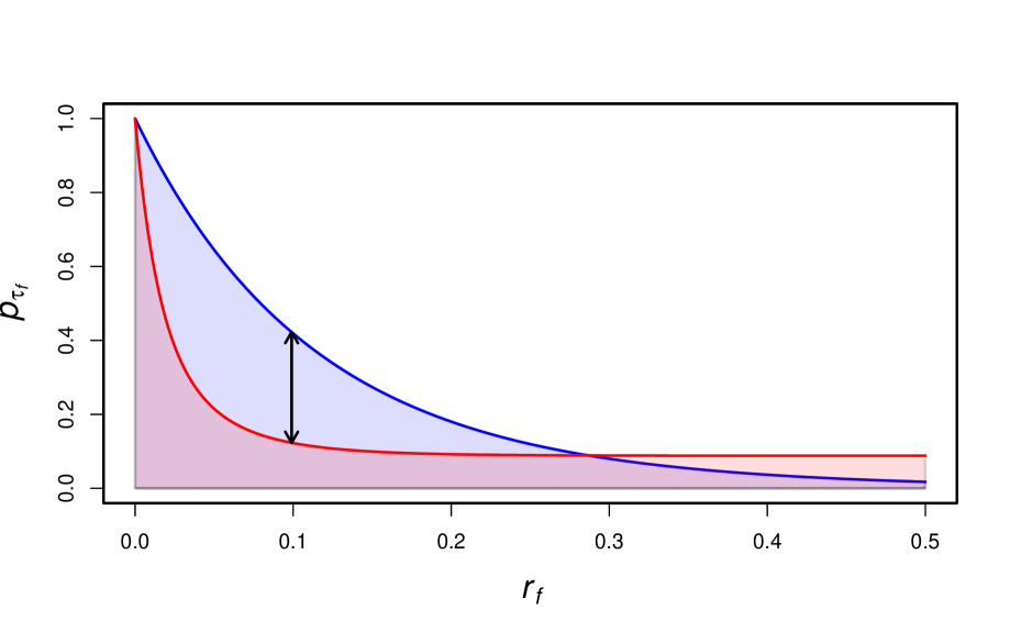
Figure 5: Algorithm 2 computes the difference between $p^{*}_{\tau_{f}}(r_{f})$ in the population that we wish to model (blue) and a simulated population of smaller size (red) and bounds the difference in the probability of identity in the simulated and model populations. $\delta_{I}$ represents the maximum difference between the area under the red curve and the area under the blue curve that is acceptable in simulations. $\delta_{p}$ represents the maximum difference between the red and blue curves that is acceptable over all values of $r_{f}$ (represented by the black arrow). Qualitatively, $\delta_{I}$ constrains the overall diversity in the simulated sequences, while $\delta_{p}$ constrains the shape of the probability of common ancestry during a sweep as a function of recombination distance.

4.3 Robust parameter rescaling for RHH simulations

Using the results in the previous section, we modify Algorithm 1 to guard against violating the assumptions of the RHH model as we rescale the parameters of the simulations.

Let $N_{1}$, $L_{1}$, etc., be defined as in the previous section. Our goal is to reduce $N_{0}$ as much as possible without altering the underlying dynamical process by more than a prespecified amount. Let $\delta_{I}$ be the maximum deviation between $I^{*}_{\alpha,s}$ for a population of size $N_{1}$ and the model population of size $N_{0}$ that we are willing to accept in our simulations. For example, let $\delta_{I}=0.01$ if we desire simulated sequences in which $I^{*}_{\alpha,s}$ in a population of size $N_{1}$ differs by no more than 1% from a population of size $N_{0}$. Let $\delta_{p}$ be the maximum difference between $p^{*}_{\tau_{f}}(u)$ in populations of size $N_{0}$ and $N_{1}$ that we are willing to accept in our simulations, over all $u$ from $0$ to $u^{*}$, the length of the flanking region. Qualitatively, $\delta_{I}$ is a constraint on the total area under $p^{*}_{\tau_{f}}(u)$, which influences the overall level of diversity, while $\delta_{p}$ is a constraint on the shape of $p^{*}_{\tau_{f}}(u)$, which influences the coalescent dynamics for a substitution that occurs at a given distance from the neutral locus. See Figure 5 for a pictorial explanation. We formalize these constraints in Algorithm 2. Note that every parameter chosen by Algorithm 2 is exactly with consistent Algorithm 1, but in Algorithm 2 we precompute how small we can make $N$ without altering the dynamics of the RHH model.

procedure Algorithm 2($\rho_{0},\alpha_{0},L_{0},N_{0},\lambda_{0},L_{1},\delta_{I},\delta_{p}$)

     Let $s_{0}=\frac{\alpha_{0}}{2N_{0}}$; $r_{0}=\frac{\rho_{0}}{4N_{0}}$; $a=\frac{s_{0}}{L_{0}r_{0}}$; $u_{max}=\nicefrac{{2}}{{a}}$

     $\alpha_{1}=\alpha_{0}=\alpha$

     Numerically solve $\frac{I_{\alpha,s0}-I_{\alpha,s1}}{I_{\alpha,s0}}=\delta_{I}$ for the quantity $s_{1}$.

     $D$ = Max[$p^{*}_{\tau_{f},s_{0}}(u)-p^{*}_{\tau_{f},s_{1}}(u)$] over all $u$ on [0,$u_{max}$]

     if $D>\delta_{p}$ then Numerically solve Max[$p^{*}_{\tau_{f},s_{0}}(u)-p^{*}_{\tau_{f},s_{1}}(u)$]=$\delta_{p}$ for $s_{1}$ over all $u$ on [0,$u_{max}$]

     end if

     $N_{1}=\frac{\alpha_{1}}{2s_{1}}$

     $r_{1}=\frac{s_{1}}{aL_{1}}$

     $\lambda_{1}=\frac{r_{1}\lambda_{0}}{r_{0}}$

     $\rho_{1}=4N_{1}r_{1}$

     return $N_{1},\rho_{1},\alpha_{1},L_{1},\lambda_{1}$

end procedure

We implemented Algorithm 2 in Python, using the numerical optimization tools in SciPy (Jones et al. 2001–) for the numerical optimization steps. In Figures 3D-F, we demonstrate the performance of Algorithm 2 for three different values of $\delta_{I}=\delta_{p}$. Smaller values of $\delta$ generate sequences that are more closely matched to the diversity in the population of size $N_{0}$, but require a larger simulated $N_{1}$ and are hence more computationally intensive. Note that for the values of $\delta$ that we have chosen herein, only a very small change in the overall diversity is expected. While larger values of $\delta$ may be acceptable for some applications, we do not recommend large values in general because the underlying dynamics are not necessarily expected to be conserved even if the change in overall diversity is small. Indeed, small deviations in mean $\pi$ and Tajima’s D are observed for the largest value of $\delta$ with strong selection (3F).

Computational performance of the rescaled simulations is shown in Figure 11 (see Appendix).

4.4 The notion of “sufficiently distant” flanking sites

We designed Algorithm 2 to work for any given $L_{0}$ in a population of size $N_{0}$. In the RHH literature, flanking regions of $L_{0}=\frac{s}{r}$ are of particular interest because equation (3) suggests that sites that are more than $\frac{s}{r}$ base pairs from the neutral locus have no impact on the neutral site (Jensen et al., 2008), at least for small $s$. However, this result does not hold in the large $s$ regime. First, the recombination fraction is not linear in the number of base pairs of flanking sequence when $r_{f}>0.1$, and $r_{f}$ cannot exceed $0.5$, even for arbitrarily long flanking sequences. Equations (3) and (13) are functions of $\frac{r_{f}}{s}$, so as $s$ gets large ($s>0.5$) it is not possible to make compensatory linear increases in $r_{f}$. Second, the dynamics of the selected site are altered when $s$ is large, as we noted in the previous sections. In particular, (13) suggests that sites that have $r_{f}=0.5$ (unlinked sites) have a non-negligible impact on the diversity at the neutral site when $s$ is very large. Our model predicts the impact of $L_{u}$ unlinked sites to be

$$E[\nicefrac{{\pi}}{{\pi_{0}}}]=\frac{1}{1+2N\lambda L_{u}\ p^{*}_{\tau_{f}}(r_{f}=0.5)}$$ (15)

Figure 6: Simulations of RHH including only a neutral region and $L_{u}$ explicitly unlinked selected sites. $L_{u}=2000$, $\lambda=0.5\times 10^{-6}$. Points represent the mean of $4\times 10^{4}$ simulations, solid lines were calculated with equation (15) in Mathematica.

Figure 6 shows the reduction in diversity, relative to neutrality, for simulations of RHH that include a neutral region and $L_{u}$ unlinked selected sites, and no linked selected sites. Equation (15) accurately predicts the reduction in diversity for these simulations. These results highlight another problem with Algorithm 1. In Algorithm 1, we linearly increase the flanking sequence as $s$ increases. However, for large $s$, the majority of these flanking sites are essentially unlinked to the neutral locus, but can have a non-negligible impact on the neutral locus. This is fundamentally different from the dynamics in the small $s$ regime, where unlinked sites have no impact on the neutral locus.

While this result may not be intuitive, it is a natural consequence of very large values of $s$. Consider the implausible but instructive case when $s\approx 2N$. In the first generation after the selected site is introduced into the population, approximately half of the offspring are expected to be descendants of the individual with the selected site. At a locus that is unlinked to the selected site, one of the two chromosomes of the individual with the selected mutant is chosen with equal probability for each of the descendants, which causes an abrupt and marked decrease in diversity. Though this effect is more subtle in our simulations in Figure 6 (which have $1<s\ll 2N$), there is a measurable decrease in $\pi$ due to the accumulated effect of unlinked sites with large $s$.

4.5 The role of interference

In the previous sections, we have restricted our analysis to parameter regimes in which interference between selected sites is very rare, which is an assumption of the RHH model. However, one of the advantages of forward simulations is that they can be performed under conditions with high levels of interference.

Figure 7: Rescaled simulations of RHH with increasing amounts of interference. 10,000 simulations were performed for each data point. Point sizes are indicative of the amount of interference in the simulations, as measured by the fraction of selected substitutions that overlap with at least one other positively selected substituted allele while both are segregating in the population. Parameters: $\alpha=2\times 10^{3}$, $L_{0}=\frac{s_{0}}{r_{0}}=4\times 10^{6}$, $r_{0}=5\times 10^{-8}$, $N_{0}=5\times 10^{3}$.

In Figure 7, we examine the performance of Algorithm 2 with very high rates of positive selection. Note that the value of $\lambda$ on the $x$-axis is the expected value in the absence of interference in a population of size $N_{0}$, and the observed value of $\lambda$ in the simulations is slightly lower. Point sizes in Figure 7 indicate the amount of interference between selected sites, as measured by the fraction of selected substitutions that overlap with at least one other substitution while segregating in the population. This is a conservative metric for the total effect of interference because it does not include the fraction of selected sites that are lost due to competition with other selected sites.

As the rate of interference increases, the theoretical predictions of equation (13) underestimate the reduction in diversity by an increasing amount (7A, black points). This is expected because as interference increases, a smaller fraction of selected sites reach fixation, and furthermore the trajectories of the sites that fix are altered due to competition. Neither of these effects is modeled by equation (13).

More strikingly, as the rate of interference increases, the separation between the rescaled populations (green and red points) and the original population (black points) also increases. This demonstrates that Algorithm 2 does not recapitulate the expected diversity in the rescaled populations when the rate of interference is high in the population of size $N_{0}$. This result is expected when we consider that the rate of interference is a function of both the rate of substitutions and the time that selected substitutions segregate in the population before fixation. It is well known that the time to fixation is a function of both $\alpha=2Ns$ and $N$, and cannot be written naturally as a function of only one or the other. Hence, when we rescale the population with fixed $\alpha$, we necessarily change the amount of interference. We analyze this effect in more detail in the next section when we perform rescaling for two sets of parameters inferred in Drosophila.

4.6 An application to Drosophila parameters

In Figure 8, we perform rescaling with RHH parameters that are relevant to Drosophila. Macpherson et al. (2007) found evidence supporting strong selection ($s=0.01$), which occurred relatively infrequently ($\lambda=3.6\times 10^{-12}$) in a Drosophila population of size $N_{0}=1.5\times 10^{6}$. Jensen et al. (2008) found weaker ($s=0.002$), more frequent selection ($\lambda=10^{-10}$) in a population of $N_{0}=10^{6}$. Our goal is not to debate the “true” parameters, but rather to investigate the practicability of rescaling using previously inferred parameters. Assuming a flanking sequence length of $L_{0}=\nicefrac{{s_{0}}}{{r_{0}}}$ and a recombination rate of $r_{0}=2.5\times 10^{-8}$, we apply Algorithms 1 and 2 to these parameter sets and investigate the effect on diversity.

Figure 8: The reduction in diversity under previously inferred RHH parameters. Panels A and C use the parameters inferred by Macpherson et al. (2007) while panels B and D use the parameters inferred by Jensen et al. (2008). The solid curves in A and B are given by (14), and the dashed curves are given by (9). Panels C and D show the probability of interference as measured by the proportion of substitutions that are introduced while another substitution is segregating in the population. The solid curves are given by (16). The size of the points in A and B is proportional to the observed value of $p_{inter}$, which plotted in C and D. The dotted vertical lines show the value of $N$ where $\delta_{I}=\delta_{p}=0.05$.

In Figure 8A, we show that the trend in simulated diversity (solid red curve) as a function of $N$ under the Macpherson et al. (2007) parameters is correctly described by (14), which predicts that the diversity decreases at low $N$. However, the model slightly underestimates the mean diversity compared to simulations. In contrast, the model predictions of the diversity are very inaccurate under the parameters estimated by Jensen et al. (2008) (Figure 8B, solid blue curve). In both 8A and 8B, Algorithm 1 strongly alters the patterns of diversity as $N$ is decreased. The value of $N_{1}$ calculated with Algorithm 2 and $\delta_{I}=\delta_{p}=0.06$ are shown with the dotted vertical line.

Point sizes in 8A and 8B indicate the proportion of substitutions that are introduced while another substitution is on the way to fixation (as in Figure 7). While the interference is fairly mild for large values of $N$ under the parameters of Macpherson et al. (2007), the amount of interference is extreme at all values of $N$ under the Jensen et al. (2008) parameters. In both cases the amount of interference in the simulations changes as we rescale $N_{1}$.

We designed Algorithm 2 under the assumption that interference is negligible in the population of size $N_{0}$. This assumption is approximately met under the parameters of Macpherson et al. (2007), where sweeps are infrequent and overlapping sweeps are rare. However, this assumption is broken by the parameters of Jensen et al. (2008), where the rate of sweeps is more than an order of magnitude higher. As a result, the diversity is not well predicted by equation (14) at any value of $N$, and Algorithm 2 fails to generate sequences with accurate patterns of genetic diversity.

In general, it is useful to know a priori when the assumptions of the RHH model are not met as a result of high interference in a population of size $N_{0}$. Consider the probability that a positively selected substitution arises in the population while another substitution is heading towards fixation, $p_{inter}$. Under the assumption that interference is sufficiently infrequent such that the mean time to fixation and probability of fixation are not strongly altered, we can approximate $p_{inter}$ as

$$p_{inter}\approx 1-\left(1-2L\lambda\right)^{\tau_{f}}=1-\left(1-\frac{2s\lambda}{r}\right)^{\frac{2(1+s)\log{2N}}{s}}\approx\frac{4(1+s)\lambda\log{2N}}{r}$$ (16)

The probability of no substitution in a single generation is $1-2L\lambda$, and hence the probability that no new selected substitutions are introduced while a given selected mutation is on its way to fixation is $\left(1-2L\lambda\right)^{\tau_{f}}$. Supposing that $L=\frac{s}{r}$ and plugging in the expectation of $\tau_{f}$ garners the rest of the terms in the equation. The final approximation is valid for very small $\frac{2s\lambda}{r}$. Note that we do not expect (16) to hold exactly in any parameter regime because the time to fixation is actually a random variable (and furthermore, both $\tau_{f}$ and $\lambda$ are altered when interference is frequent), but we find that $p_{inter}$ is a useful approximation for describing the interference in simulations during the rescaling process.

In Figures 8C and 8D, we investigate the behavior of (16) as we rescale the population size. As $N$ is decreased from $N_{0}$, the value of $p_{inter}$ initially decreases because the product $(1+s)\log{2N}$ decreases. However, as $N$ gets very small with Algorithm 1, $(1+s)\log{2N}$ eventually begins to increase because $1+s$ increases faster than $\log{2N}$ decreases, increasing the amount of interference.

Although the exact calculation of the effects of interference is very challenging, it is straightforward to calculate the value of $p_{inter}$ in a population of size $N_{0}$. If the value of $p_{inter}$ is large (e.g., $>0.05$, as with the parameters in Figure 8B), then the assumptions of Algorithm 2 are broken and there is no guarantee that the rescaled simulated sequences will be sufficiently accurate. By contrast, if there is low interference in a population of size $N_{0}$ then it is safe to perform rescaling so long as the value of $p_{inter}$ is constrained. In practice, the value of $p_{inter}$ (or other quantities that are related to the rate of interference) can be taken as an additional constraint in the calculation of $N_{1}$ in Algorithm 2 such that the impact of interference is limited under rescaling.

5 Discussion

Simulations are an integral part of population genetics because it is often difficult to obtain exact analytical expressions for many quantities of interest, such as likelihoods for sequence data under a given model. Until recently, forward simulations were not practical because of the large computational burden that they can impose. However, several new forward simulation techniques have been proposed and published (Hoggart et al. 2007; Hernandez 2008; Zanini and Neher 2012; Aberer and Stamatakis 2013; Messer 2013), and their use in population genetic studies is becoming increasingly popular.

Despite these computational advances, it remains very computationally intensive to simulate large populations and long chromosomes in a forward context. It is frequently necessary to perform parameter rescaling to achieve computational feasibility for parameter regimes of interest (e.g., $N>10^{5}$ with long flanking sequences), particularly for applications such as Approximate Bayesian Computation which require millions of simulations for accurate inference. The hope of such rescaling efforts is that expected patterns of diversity will be maintained after rescaling, and that the underlying genealogical process will remain unaltered.

In this investigation, we tested a “naive” approach to parameter rescaling, and showed that this approach can strongly alter the expected patterns of diversity because it does not conserve the underlying genealogical process at the neutral site. In particular, for fixed values of $\alpha$, $s$ can get arbitrarily large as $N$ is decreased, and previous theoretical results do not accurately predict the patterns of diversity in this parameter regime. We derived a new theoretical form for the reduction in diversity when $s$ is large, and show that it has strong predictive power in simulations. We leveraged this result to develop a simple rescaling scheme (Algorithm 2) that approximately conserves the underlying genealogical process. We note that in practice Algorithm 2 may not always be necessary, and as long as $s$ remains small (say, $<0.1$) Algorithm 1 will suffice. The advantage of Algorithm 2 is that it allows us to quantitate the effect of rescaling, and to get the best possible computational performance for a given error tolerance.

It will be of great interest to extend the rescaling results for recurrent sweeps presented herein to models that include arbitrary changes in population size and interference between selected sites. In the case of changes in population size, we note that the strategy presented in Algorithm 2 can be easily extended to perform optimization across a range of population sizes such that the constraints are simultaneously satisfied at all time points in a simulation. This strategy is consistent with previous approaches to rescaling in the context of complex demography (Hoggart et al., 2007).

Interference poses a greater challenge, because the amount of interference is dependent both on the rate of substitution and the time that selected sites segregate. It is well known that the time to fixation of selected alleles cannot be written as a simple function of $\alpha$ and depends on $N$ as well, and hence rescaling population size with fixed $\alpha$ alters the effects of interference on sequence diversity (Comeron and Kreitman, 2002). Improved understanding of scaling laws for interference may be necessary in order to develop appropriate rescaling strategies, to the extent that such rescaling is possible at all in a forward simulation context. However, recent progress was made in the case of very strong interference, where scaling laws were recently derived by Weissman and Barton (2012).

The rescaling results presented here pose an interesting dilemma for the use of forward simulations in population genetic studies, as previously noted by Kim and Wiehe (2009). A major appeal of forward simulations (as compared to coalescent simulators) is the ability to incorporate arbitrary models (e.g., interference between selected sites, complex demographic processes) without knowing anything about the distribution of sample paths a priori. However, if simulations are only feasible when the parameters are rescaled, there is no guarantee for any given theoretical model that the rescaling will maintain expected dynamics. We also note that the rescaling method proposed herein was informed by in-depth knowledge provided by the previous work of several authors, and that in general it may not always be obvious which parameters must be simultaneously adjusted to maintain expected patterns of variation in simulations for a given complex model.

Nonetheless, forward simulation in population genetics has a bright future. Forward simulation remains the only way to simulate arbitrarily complex models. For many populations of interest (e.g., ancestral human populations), population size is sufficiently small such that it can often be directly simulated without rescaling. Continued computational advances in both hardware and software in coming years will expand the boundaries of computational performance of forward simulation. Finally, active development of the theory of positive selection, interfering selected sites, background selection, demographic processes, and the joint action thereof will lend further insight into parameter rescaling and advances in the use of forward simulations in population genetic studies.

6 Appendix

6.1 Derivation of $p^{*}_{\tau_{f}}$ for large $s$

In this section, we solve for the probability of identity $p_{\tau_{f}}$ when the selection coefficient is large. We will be concerned with the probability of identity $p$ at various frequencies throughout the sweep process. We will subscript $p$ with $t(x)$ to indicate the value of $p$ at the time when the selected site reaches frequency $x$ (e.g., $p_{t(\nicefrac{{1}}{{2N}})}$). The trajectory of the selected site for large $s$ is given (12), while the dynamics of the neutral site are given by (2). We transform (2) into allele frequency space by dividing by (12). We obtain:

$$\frac{d}{dx}p=\frac{(1-p)(1+2sx)}{2Nsx^{2}(1-x)}-\frac{2r_{f}p(1+2sx)}{sx}$$ (17)

This equation can be solved in Mathematica with the initial condition $p_{t(\nicefrac{{1}}{{2N}})}=1$, meaning that all backgrounds carrying the selected locus are identical at the neutral locus when the selected site is introduced. At the end of the sweep, $x\approx 1$. We take the solution with $x=1-\nicefrac{{1}}{{2N}}$ because $x=1$ results in a singularity.

$$\begin{split}p_{\tau_{f}}&=e^{2r_{f}(-2+\frac{1}{2N})+\frac{2N-2}{s-2Ns}}\left(2-\frac{1}{N}\right)^{-\frac{1+2Nr_{f}+2s}{Ns}}\left(\frac{1}{N}\right)^{\frac{2+\nicefrac{{1}}{{s}}}{2N}}\\ &\left(e^{\frac{2r_{f}}{N}}\left(\frac{1}{N}\right)^{\frac{1+4Nr_{f}+2s}{2Ns}}\right.+4^{\frac{r_{f}}{s}}e^{\frac{1}{s}}\left(2-\frac{1}{N}\right)^{\frac{2+\frac{1}{s}}{2N}}\\ &\left(\int_{1}^{1-\frac{1}{2N}}\frac{e^{\frac{\frac{1}{C}-8Nr_{f}sC+(1+2s)\log[1-C]-(1+4Nr_{f}+2s)\log[C]}{2Ns}}\left(-1+2sC\right)}{2Ns\left(-1+C\right)C^{2}}dC\ \right.\\ &\left.\left.-\int_{1}^{\frac{1}{2N}}\frac{e^{\frac{\frac{1}{C}-8Nr_{f}sC+(1+2s)\log[1-C]-(1+4Nr_{f}+2s)\log[C]}{2Ns}}\left(-1+2sC\right)}{2Ns\left(-1+C\right)C^{2}}dC\right)\right)\end{split}$$ (18)

Equation (18) can be numerically integrated in Mathematica. However, this solution is complicated, slow to evaluate, and provides little intuition about the dynamics. As an alternative, we employ an approximate solution strategy.

Following Barton (1998) and others, we subdivide the trajectory of the selected allele into low frequency and high frequency portions. For small $x$, the term $(1+2sx)\approx 1$, even for large $s$. As a result, there is little difference between the dynamics for small $s$ and large $s$ sweeps at low frequency. We rewrite (17) as

$$\frac{d}{dx}p=\frac{(1-p)}{2Nsx^{2}(1-x)}-\frac{2r_{f}p}{sx}$$ (19)

which is valid for low $x$. We define the solution to (19) on the interval $x=[\nicefrac{{1}}{{2N}},\epsilon]$ as $p_{t(\epsilon)}$.

For $x>\epsilon$, the second term on the RHS of (17) dominates the first term, because the first term is inversely proportional to the number of selected chromosomes. To obtain the high frequency dynamics of the selected allele, we take $p_{t(\epsilon)}$ as the initial condition and solve the following differential equation on the interval $x=[\epsilon,1]$:

$$\frac{d}{dx}p=-\frac{2r_{f}p(1+2sx)}{sx}$$ (20)

We find the solution:

$$p_{\tau_{f}}=\left(e^{4r_{f}(\epsilon-1)}\right)\epsilon^{\frac{2r_{f}}{s}}p_{t(\epsilon)}$$ (21)

We can perform the exact same analysis under the assumption that the dynamics are given by $\frac{dx(t)}{dt}=sx(t)(1-x(t))$, as was done by SWL. This garners the solution:

$$p^{SWL}_{\tau_{f}}=\epsilon^{\frac{2r_{f}}{s}}p_{t(\epsilon)}$$ (22)

which differs by only a factor of $e^{4r_{f}(\epsilon-1)}$ from (21). Since (22) was derived under assumptions identical to those used in Stephan et al. (1992), we conclude that sweeps with large $s$ can be modeled with the equation

$$p_{\tau_{f}}=e^{-4r_{f}}\left(1-\frac{2r_{f}}{s}\alpha^{\frac{-2r_{f}}{s}}\Gamma\left[\frac{-2r_{f}}{s},\frac{1}{\alpha}\right]\right)$$ (23)

This equation provides very similar results to (3) for small $s$, as expected, but deviates for large $s$ (Figure 9).

Figure 9: Equation (23) (blue) and Equation (18) (black) compared to (3) (red). As expected, (23) and (3) are in very close agreement for small $s$, but diverge for large $s$. Equation (23) is a good approximation to (18) across a wide range of values of $s$. $\alpha=10^{4}$

To verify that this approximation provides accurate results to the full solution given by equation (18), we compared (18) to (23) in Mathematica. Agreement is very good between the exact and approximate solutions for all values of $s$ that we investigated (Figure 9).

6.2 RHH simulations in SFS_CODE

We performed forward simulations of RHH with SFS_CODE (Hernandez 2008). An example command line for a RHH simulation is:

sfs_code 1 10 -t <$\theta$> -Z -r <$\rho$> -N <$N$> -n <$n$> -L 3 <$L$> <$l_{0}$> <$L$> -a N R -v L A 1 -v L 1 <$R_{mid}$> -W L 0 1 <$\alpha$> 1 0 -W L 2 1 <$\alpha$> 1 0

All of these options are described in the SFS_CODE manual, which is freely available online at sfscode.sourceforge.net, or by request from the authors. Briefly, this command line runs 10 simulations of a single population of size $N$ and samples $n$ individuals at the end. The recombination rate is set to $\rho$, and 3 loci are included in the simulation. The middle locus (locus 1) is $l_{0}$ base pairs long while the flanking loci are $L$ bp long. The middle locus is neutral, while the flanking loci contain selected sites with selection strength $\alpha=2Ns$. Every mutation in the flanking region is positively selected. The sequence is set to be non-coding with the option “-a N r”. The “-v” option provides the flexibility to designate different rates of mutation at different loci, and the mechanics of its usage are described in detail in the SFS_CODE manual. $R_{mid}$ specifies the rate at which mutations are introduced into the middle segment relative to the flanking sequences. Please see the SFS_CODE manual for a detailed example of parameter choice for RHH simulations.

Forward simulations of DNA sequences can require large amounts of RAM and many computations. Recurrent hitchhiking models are particularly challenging to simulate because very long sequences must be simulated. In particular, for a given selection coefficient $s$, RHH theory suggests that sites as distant as $r_{f}\approx s$ must be included in the simulation to include all sufficiently distant sites (see (3)).

In many organisms, $r\approx 10^{-8}$. Assuming $r_{f}\approx rL$, this implies that a selection coefficient of $s=0.1$ would require $10^{7}$ base pairs of simulated sequence on each side of the neutral locus in order to include all possible impactful sites. This is a prohibitively large amount of sequence for many reasonably chosen values of $\theta$ and $N$ in forward simulations (Figure 10). However, in simulations of RHH, we are primarily interested in examining the diversity at a short, neutral locus. We adapted SFS_CODE such that individual loci can have different mutation rates and different proportions of selected sites. For RHH simulations, we set the proportion of selected sites to zero in the neutral locus, and 1 in the flanking sequence. This greatly increases the speed and decreases RAM requirements for SFS_CODE because much less genetic diversity is generated in the flanking sequences (Figure 10, blue curves). Time and RAM usage were measured with the Unix utility “time” with the command “/usr/bin/time -f ‘%e %M’ sfs_code [options]”. Note that time reports a maximum resident set size that is too large by a factor four due to an error in unit conversion on some platforms, which we have corrected herein. Simulations were performed on the QB3 cluster at UCSF, which contains nodes with a variety of architectures and differing amounts of computational load at any given time. As such, the estimates of efficiency herein should be taken only as qualitative observations.

6.3 Efficiency of rescaled simulations

We report the time to completion of rescaled simulations relative to non-scaled populations using Algorithm 2 (Figure 11). We observe reductions in time between approximately 99% and 40% for the parameters under consideration here. In general, the best performance is obtained for weaker selection, since in this case $s$ is small in the population of size $N_{0}$, meaning that the value of $N$ can be changed quite dramatically without breaking the small $s$ approximation. Better gains are also observed as the error threshold is increased, but this comes at an accuracy cost (see section 4.3).

Figure 10: The computational burden of simulations of recurrent positive selection in SFS_CODE is much lower in the new version of SFS_CODE. Both RAM requirements and time to complete the simulations are reduced. Points represent the mean of 500 simulations. $\theta=10^{-3}$, $\rho=10^{-3}$, $N=500$, $\lambda=10^{-9}$, $\alpha=1000$.

Figure 11: Duration of rescaled simulations ($t(N_{1})$) relative to non-scaled simulations ($t(N_{0})$). Parameters were chosen to match Figure 3. Parameters: $N_{0}=5\times 10^{3}$, $\rho_{0}=10^{-3}$, $\lambda_{0}=10^{-10}$, $L_{0}=10^{6}$, $L_{1}=10^{5}$.

7 Acknowledgments

This work was partially supported by the National Institutes of Health (grants P60MD006902, UL1RR024131, 1R21HG007233, 1R21CA178706, and 1R01HL117004-01 to R.D.H.), an ARCS foundation fellowship (L.H.U.), and National Institutes of Health training grant T32GM008155 (L.H.U.). We thank John Pool for stimulating discussion that motivated this research and Zachary A. Szpiech, Raul Torres, M. Cyrus Maher, Kevin Thornton, Joachim Hermisson, and two anonymous reviewers for comments on the manuscript.

References

- Aberer and Stamatakis (2013) Aberer, A. J., and A. Stamatakis, 2013 Rapid forward-in-time simulation at the chromosome and genome level. BMC Bioinformatics 14: 216–216.
- Arbiza et al. (2013) Arbiza, L., I. Gronau, B. A. Aksoy, M. J. Hubisz, B. Gulko, et al., 2013 Genome-wide inference of natural selection on human transcription factor binding sites. Nat Genet 45: 723–729.
- Bachtrog (2008) Bachtrog, D., 2008 Similar rates of protein adaptation in drosophila miranda and d. melanogaster, two species with different current effective population sizes. BMC Evol Biol 8: 334–334.
- Barrett et al. (2006) Barrett, R. D., R. C. MacLean, and G. Bell, 2006 Mutations of intermediate effect are responsible for adaptation in evolving pseudomonas fluorescens populations. Biol Lett 2: 236–238.
- Barton (1998) Barton, N. H., 1998 The effect of hitch-hiking on neutral genealogies. Genetics Research 72: 123–133.
- Beaumont et al. (2002) Beaumont, M. A., W. Zhang, and D. J. Balding, 2002 Approximate bayesian computation in population genetics. Genetics 162: 2025–2035.
- Bustamante et al. (2005) Bustamante, C. D., A. Fledel-Alon, S. Williamson, R. Nielsen, M. T. Hubisz, et al., 2005 Natural selection on protein-coding genes in the human genome. Nature 437: 1153–1157.
- Chevin et al. (2008) Chevin, L.-M., S. Billiard, and F. Hospital, 2008 Hitchhiking both ways: effect of two interfering selective sweeps on linked neutral variation. Genetics 180: 301–316.
- Comeron and Kreitman (2002) Comeron, J. M., and M. Kreitman, 2002 Population, evolutionary and genomic consequences of interference selection. Genetics 161: 389–410.
- Coop and Ralph (2012) Coop, G., and P. Ralph, 2012 Patterns of neutral diversity under general models of selective sweeps. Genetics 192: 205–224.
- Crisci et al. (2012) Crisci, J. L., Y.-P. Poh, A. Bean, A. Simkin, and J. D. Jensen, 2012 Recent progress in polymorphism-based population genetic inference. Journal of Heredity 103: 287–296.
- Cutter and Payseur (2013) Cutter, A. D., and B. A. Payseur, 2013 Genomic signatures of selection at linked sites: unifying the disparity among species. Nat Rev Genet 14: 262–274.
- Fisher (1999) Fisher, R. A., 1999 The genetical theory of natural selection: a complete variorum edition. Oxford University Press.
- Haldane (1919) Haldane, J., 1919 The combination of linkage values and the calculation of distances between the loci of linked factors. Journal of Genetics 8: 299–309.
- Hernandez (2008) Hernandez, R. D., 2008 A flexible forward simulator for populations subject to selection and demography. Bioinformatics 24: 2786–2787.
- Hoggart et al. (2007) Hoggart, C. J., M. Chadeau-Hyam, T. G. Clark, R. Lampariello, J. C. Whittaker, et al., 2007 Sequence-level population simulations over large genomic regions. Genetics 177: 1725–1731.
- Ingvarsson (2010) Ingvarsson, P. K., 2010 Natural selection on synonymous and nonsynonymous mutations shapes patterns of polymorphism in populus tremula. Mol Biol Evol 27: 650–660.
- Jensen et al. (2008) Jensen, J. D., K. R. Thornton, and P. Andolfatto, 2008 An approximate bayesian estimator suggests strong, recurrent selective sweeps in drosophila. PLoS Genet 4.
- Jones et al. (2001–) Jones, E., T. Oliphant, P. Peterson, et al., 2001– SciPy: Open source scientific tools for Python.
- Kaplan et al. (1989) Kaplan, N. L., R. R. Hudson, and C. H. Langley, 1989 The ”hitchhiking effect” revisited. Genetics 123: 887–899.
- Kim and Stephan (2003) Kim, Y., and W. Stephan, 2003 Selective sweeps in the presence of interference among partially linked loci. Genetics 164: 389–398.
- Kim and Wiehe (2009) Kim, Y., and T. Wiehe, 2009 Simulation of dna sequence evolution under models of recent directional selection. Briefings in Bioinformatics 10: 84–96.
- Kimura (1962) Kimura, M., 1962 On the probability of fixation of mutant genes in a population. Genetics 47: 713–719.
- Macpherson et al. (2007) Macpherson, J. M., G. Sella, J. C. Davis, and D. A. Petrov, 2007 Genomewide spatial correspondence between nonsynonymous divergence and neutral polymorphism reveals extensive adaptation in drosophila. Genetics 177: 2083–2099.
- Maher et al. (2012) Maher, M. C., L. H. Uricchio, D. G. Torgerson, and R. D. Hernandez, 2012 Population genetics of rare variants and complex diseases. Hum Hered 74: 118–128.
- Messer (2013) Messer, P. W., 2013 Slim: Simulating evolution with selection and linkage. Genetics .
- Ota and Kimura (1975) Ota, T., and M. Kimura, 1975 The effect of selected linked locus on heterozygosity of neutral alleles (the hitch-hiking effect). Genet Res 25: 313–326.
- Pool et al. (2010) Pool, J. E., I. Hellmann, J. D. Jensen, and R. Nielsen, 2010 Population genetic inference from genomic sequence variation. Genome Res 20: 291–300.
- Singh et al. (2013) Singh, N. D., J. D. Jensen, A. G. Clark, and C. F. Aquadro, 2013 Inferences of demography and selection in an african population of drosophila melanogaster. Genetics 193: 215–228.
- Smith and Haigh (1974) Smith, J. M., and J. Haigh, 1974 The hitch-hiking effect of a favourable gene. Genetics Research 23: 23–35.
- Stephan et al. (2006) Stephan, W., Y. S. Song, and C. H. Langley, 2006 The hitchhiking effect on linkage disequilibrium between linked neutral loci. Genetics 172: 2647–2663.
- Stephan et al. (1992) Stephan, W., T. H. Wiehe, and M. W. Lenz, 1992 The effect of strongly selected substitutions on neutral polymorphism: Analytical results based on diffusion theory. Theoretical Population Biology 41: 237 – 254.
- Torgerson et al. (2009) Torgerson, D. G., A. R. Boyko, R. D. Hernandez, A. Indap, X. Hu, et al., 2009 Evolutionary processes acting on candidate cis-regulatory regions in humans inferred from patterns of polymorphism and divergence. PLoS Genet 5.
- Weissman and Barton (2012) Weissman, D. B., and N. H. Barton, 2012 Limits to the rate of adaptive substitution in sexual populations. PLoS Genet 8.
- Wiehe and Stephan (1993) Wiehe, T. H., and W. Stephan, 1993 Analysis of a genetic hitchhiking model, and its application to dna polymorphism data from drosophila melanogaster. Mol Biol Evol 10: 842–854.
- Wolfram (2010) Wolfram, 2010 Mathematica edition: Version 8.0.
- Zanini and Neher (2012) Zanini, F., and R. A. Neher, 2012 Ffpopsim: an efficient forward simulation package for the evolution of large populations. Bioinformatics 28: 3332–3333.