Veni Vidi Vici, A Three-Phase Scenario For Parameter Space Analysis in Image Analysis and Visualization

Abstract

Automatic analysis of the enormous sets of images is a critical task in life sciences. This faces many challenges such as: algorithms are highly parameterized, significant human input is intertwined, and lacking a standard meta-visualization approach. This paper proposes an alternative iterative approach for optimizing input parameters, saving time by minimizing the user involvement, and allowing for understanding the workflow of algorithms and discovering new ones. The main focus is on developing an interactive visualization technique that enables users to analyze the relationships between sampled input parameters and corresponding output. This technique is implemented as a prototype called Veni Vidi Vici, or ”I came, I saw, I conquered.” This strategy is inspired by the mathematical formulas of numbering computable functions and is developed atop ImageJ, a scientific image processing program. A case study is presented to investigate the proposed framework. Finally, the paper explores some potential future issues in the application of the proposed approach in parameter space analysis in visualization.

1 Introduction

Visual analysis is a vital tool in life sciences. Scientists can automate experiments and capture large result sets of digital images [1]. Automatic analysis of the enormous sets of biomedical images is a must. Algorithms and techniques of image analysis are highly parameterized and significant human input is intertwined to optimize parameter settings [2]. It is common to utilize machine-learning algorithms in minimizing user overhead. However, users are asked to determine objects of interest in some input images, then the algorithms create classifiers to recognize similar objects in other images. This approach highly relies on the experience of domain experts and it requires a great amount of object labeling to be done by hand.

Also, lacking a standard meta-visualization[3] approach is a challenge. High-level description of a visualization algorithm can not be gained by debugging, forcing developers of the algorithm to manually create high-level illustrations to understand the workflow of the algorithm.

This paper proposes an alternative iterative approach for optimizing input parameters, saving time by minimizing the user involvement, and allowing for understanding the workflow of algorithms and discovering new ones. The main focus is on developing an interactive visualization technique that enables users to analyze the relationships between sampled input parameters and corresponding output. This technique is implemented in a prototype called Veni Vidi Vici , following the famous Latin sentence claimed to be said by Julius Caesar [4] . It translates as ”I came, I saw, I conquered.” This strategy is inspired by the mathematical formulas of numbering computable functions [5] and is developed atop ImageJ [6], a scientific biomedical image analysis program.

Section 2 summarizes related work, before surveying ImageJ in Section 3. Proposed work is presented in Section 4. This includes explaining Veni Vidi Vici strategy (Section 4.1), presenting the underpinning mathematical foundations (Section 4.2), and implementing the framework as a custom plug-in for ImageJ (Section 4.3). Evaluation of the proposed approach with case studies are shown in Section 5. Finally, presenting conclusion and outlining future work in Section 6.

2 Related Work

Many visualization techniques are proposed to facilitate investigating the relationships between parameters and outcomes. Linked charts are among the first attempts to use interactive visualization to parameter optimization [7]. The mapping $p_{1},...,p_{n}$ $\to$ $o_{1},...,o_{m}$, where $p_{1},...,p_{n}$ are the parameters and $o_{1},...,o_{m}$ are the outcomes, can be represented as n + m interactive histograms. This approach is then extended to prosection matrices [8]. An alternative approach is proposed for visualizing the parameter search process as a directed graph [9].

Exploration graphs for history management are used in VisTrails visualization management system [10]. The exploration is still linear and time consuming. This can be partially improved by allowing users to write code snippets to perform iterations over parameter values [11].

Many techniques are proposed for image-based analysis and visualization as a structured gallery [12]. An innovative technique is proposed based on preset based interaction with high dimensional parameter spaces [13]. A preset is a reference point in parameter space used to compute the outcome by calculating the linear combination of the inverse distances from the preset to the outcome.

Many successful analysis and visualization systems are available such as IRIS Explorer[14]. CellProfiler [15] is an image analysis software for identifying and quantifying cell phenotypes. VolumeShop [16] is an interactive system for direct volume illustration.

Vismon [17] is a data analysis visual tool for fisheries to enable decision makers to quickly narrow down all possible management options to an agreeable small set. A risk assessment framework for chum salmon is developed to evaluate different management policies [19]. A detailed trade-off among the few chosen management options can be performed [18].

Most of previous systems are domain-specific. However, some are for a wide range of applicability. Tuner [20] is an application for finding optimal parameter settings for complex algorithms in high-dimensional parameter space. It supports sampling, re-sampling, and visually seeing the stability of certain parameter settings with respect to the objective measures.

For more wisdom on new trends in visualization pipeline, algorithmic stability, and the exploration of parameters, readers are encouraged to check IEEE VisWeek 2012 tutorial on ”Uncertainty and Parameter Space Analysis in Visualization” [21].

3 ImageJ

ImageJ [6] is a free image processing program developed at the National Institutes of Health. Originally, it is designed to be used by biomedical researchers working with microscope images and videos.

Being based on Java which supports algorithmic digital image processing[22], ImageJ is designed with an open architecture that provides extensibility via Java plugins and recordable macros[23]. These plugins provide custom solution for many analysis and visualization problems such as:

• three-dimensional live-cell imaging[24],

• to radiological image processing[25],

• multiple imaging system data comparisons[26],

• automated hematology systems[27], and

• Visualizing multidimensional biological image data[28].

The following four subsections show a comprehensive list of plugins.

3.1 Analysis

• Autocorrelation,

• MRI t2 calculations,

• Line Analyzer,

• Image Correlator ,

• Particle Remover,

• Circularity ,

• Modulation Transfer Function,

• Specify ROI ,

• Specify Line Selection,

• 16-bit Histogram ,

• Draw line or point grids ,

• Moment Calculator ,

• Batch Statistics ,

• Cell Counter ,

• Oval Profile Plot ,

• Color Comparison ,

• Radial Profile Plot ,

• Microscope Scale ,

• MRI Analysis Calculator ,

• Sync Measure 3D ,

• Hough Circles ,

• Convex Hull, Circularity, Roundness ,

• Fractal Dimension and Lacunarity ,

• Measure And Label ,

• Colocalization ,

• Granulometry ,

• Texture Analysis ,

• Named Measurements ,

• Cell Outliner ,

• Grid Cycloid Arc ,

• RGB Profiler ,

• Colocalization Finder ,

• Spectrum Extractor ,

• Contact Angle ,

• RG2B Colocalization ,

• Color Profiler ,

• Hull and Circle ,

• MR Urography ,

• Template Matching ,

• Extract IMT from ultrasound images ,

• ITCN (Image-based Tool for Counting Nuclei) ,

• Multi Cell Outliner ,

• FRETcalc - FRET by acceptor photobleaching ,

• JACoP (Just Another Colocalization Plugin),

• FRET and Colocalization Analyzer ,

• CASA (Computer Assisted Sperm Analyzer) ,

• Radial Profile Plot Extended ,

• Concentric Circles (non-destructive overlay),

• Azimuthal Average ,

• Slanted Edge Modulation Transfer Function,

• Calculate 3D Noise ,

• FWHM (analyze photon detector pinhole images),

• SSIM index (calculate structural similarity),

• Image Moments (image moments of n-th rank) ,

• MS SSIM index (multi-scale structural similarity),

• Colony Counter (count colonies in agar plates),

• Levan (chromosome morphology) ,

• EXTRAX (electron diffraction intensity extraction),

• Fractal Surface Measurement ,

• Foci Picker3D (finds local maxima in 2D and 3D images),

• Diameter (measures the diameter of a blood vessels),

• Graph Demo (creates particle adjacency lists) ,

• Asymmetry Analysis (HR-TEM image conditions) ,

• 2D NMR Analysis (integrates peaks in 2D NMR spectra) ,

• MetaData and Intracellular Calcium Line Scan Analysis,

• GHT (General Hough Transformation object recognition),

• IntraCell (nanoparticle colocalization within cells),

• Lemos Asymmetry Analysis (dental panoramic radiographs),

• Merz Grid Macro (semicircular lines and points in overlay),

• Stress Granule Counter (counts SGs in eucaryotic cells),

• Vamp 2D and 3D (isolate puncta in 2D and 3D images) ,

• Sampling Window (unbiased sampling window) ,

• Map Bone Microstructure (histomorphometry parameters),

• Results and Text ,

• Comment Writer

3.2 Filters

• Real Convolver

• Fast Fourier Transform (FFT)

• LoG Filtering

• Background Subtraction and Normalization

• Contrast Enhancer

• Background Correction

• Byte Swapper

• Discrete Cosine Transform (DCT)

• FFT Filter

• FFTJ and DeconvolutionJ

• Unpack 12-bit Images

• De-interlace

• 2D Gaussian Filter

• Kalman Filter

• Dual-Energy Algorithm

• Anisotropic Diffusion (edge-preserving noise reduction)

• Grayscale Morphology

• 2D Hybrid Median Filter

• 3D Hybrid Median Filter

• Spectral Unmixing

• Haar Wavelet Filter and Adaptive Median Filter

• ’A trous’ Wavelet Filter

• Kuwahara Filter

• Granulometric Filtering

• Windowed-Sinc Filter (low pass time series filter)

• Anisotropic Diffusion 2D (edge-preserving noise reduction)

• Auto Gamma for gamma correction

• Linearize Gel Data

• Radon Transform (back projection, sinogram)

• Correct X Shift of Confocal Images

• Multi Otsu Threshold

• Spectral Unmixing of Bioluminescence Signals

• Lipschitz Filter

• Float Morphology (erode, dilate, open, close)

• X Shifter (correct pixel mismatch of confocal images)

• Sigma Filter (edge-preserving noise reduction)

• Rolling Ball Background Subtraction

• Mean Shift Filter (edge-preserving smoothing)

• Accurate Gaussian Blur

• Add Poisson Noise

• CLAHE (Contrast Limited Adaptive Histogram Equalization)

• Floyd Steinberg Dithering

• Polar Transformer (corrects radial and angular distortions)

• Gaussian Blur 3D

• Image Rotator (rotates image around ROI center of mass)

• Mexican Hat (2D Laplacian of Gaussian)

3.3 Segmentation

• Mixture Modeling Thresholding ,

• Otsu Thresholding ,

• Watershed Segmentation Maximum Entropy Thresholding ,

• MultiThresholder (IsoData, MaxEntropy, Otsu, etc),

• Multi Otsu Threshold ,

• SIOX (Simple Interactive Object Extraction),

• RATS (Robust Automatic Threshold Selection) ,

• Densitometry ,

• Blob Labeler (labels connected blobs of pixels)

3.4 Collections

• UCSD Confocal Microscopy Plugins ,

• MBF ImageJ for Microscopy Collection

4 Proposed Framework

4.1 Veni Vidi Vici

Let us discuss the general idea behind the proposed new iterative approach for optimizing input parameters and allowing for understanding the workflow of algorithms and discovering new ones. The main focus is on developing an interactive visualization technique that enables users to analyze the relationships between sampled input parameters and corresponding output. This technique is implemented in a prototype called Veni Vidi Vici , following the famous Latin sentence claimed to be said by Julius Caesar [4]. It translates as ”I came, I saw, I conquered.”

It falls into three main parts:

• Veni: corresponds to analysis and user interaction,

• Vidi: corresponds to visualization, and

• Vici: corresponds to segmentation or similar tasks.

Figure 1 shows the schematic diagram of the proposed strategy.

Figure 1: Proposed Framwork

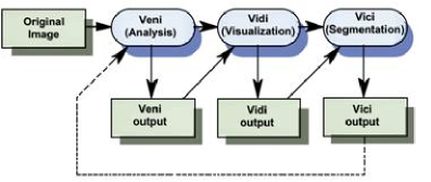
Note that rectangles represent files and rounded rectangles represent processes. Veni takes the original image and the outcome of previous runs as input. The dashed line is not presented in the first run. User interaction is minimized to Veni. Vidi is sandwiched between the other two processes. Vici corresponds to a desired task to perform on the image such as segmentation or counting objects. The final outcome is then fed-back to Veni. These three processes are optional ,i.e. any one can be skipped, with at least one applied.

4.2 Mathematical Foundations

Recall that the over all process involves a set of n parameters: $p_{1},...,p_{n}$. Assume that these n parameters are divided among the three processes of Veni, Vidi, and Vici. Assume that $a,b,$ and $c$ are the parameter shares of Veni, Vidi, and Vici respectively. So, $n=a+b+c$. Veni, Vidi, and Vici are descried mathematically in table 1.

Table 1: Parameter share

Operation	Summary
Veni(g, $x_{1},...,x_{a}$)	Apply Veni on images g, setting its a parameters to x’s values
Vidi(g, $y_{1},...,y_{b}$)	Apply Vidi on images g, setting its b parameters to y’s values
Vici(g, $z_{1},...,z_{c}$)	Apply Vici on images g, setting its c parameters to z’s values

The proposed strategy for exploring parameter space is inspired by the mathematical formulas of numbering computable functions [5]. Let us define some functions that allow us to map any set of Veni, Vidi, and Vici to a unique code, or Gödel number [29].

Mapping ordered pairs to N

A function $\pi$ such that $\pi(x,y)=2^{x}(2y+1)-1$ maps $N^{2}\to N$. That is, $\pi$ maps the ordered pair (x,y) to a single number $2^{x}(2y+1)-1$.

Figure 2: A graphical representation of $\pi$

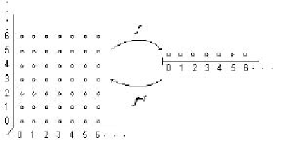
To see how this mapping is done, note that $\pi=2^{x}(2y+1)-1$ is a number such that $\pi$ has x factors of 2 and a remaining odd number 2y + 1. As an example, let $\pi$ = 103935. You can factories $\pi$ + 1 into 9 factors of 2 and you are left over with $203=101(2)-1$. Hence, $\pi+2=2^{9}(2(101)+1)$ yielding x = 9 and y = 101. Since every number has a different factorization into powers of two, $\pi$ is a bijective function mapping. The inverse of $\pi$ is defined such that $\pi_{1}$(z) returns the exponent of $p_{1}$ = 2 in the prime factorization of z, and $\pi_{2}$(z) returns the exponent of $p_{2}$ = 3.

Mapping Ordered Triples to N

A function $\zeta:N^{+}\times N^{+}\times N^{+}\to N$ maps an ordered set of three natural numbers to a single number. To define this mapping, we can use the function $\pi$, and write $\zeta(m,n,q)=\pi(\pi(m-1,n-1),q-1)$ which maps the first parameters m and n to one number using $\pi$. The resulting value and the third number q is then mapped to one number again using $\pi$. Hence, the final result is one natural number. The purpose in subtracting 1 from the parameters m,n and q is to include zero in the mapping.

Mapping a Finite Sequence $N^{k}$ to N

The concept of converting bases can be used to devise a bijection from a finite sequence of numbers to one natural number.

The binary representation is simple yet powerful. A decimal number can be converted into a binary representation by repeatedly subtracting the next largest possible power of two from the previous remainder, until no other powers exist.

Consider the conversion of 44 decimal to binary: $44=2^{5}+12=2^{5}+2^{3}+4=2^{5}+2^{3}+2^{2}$. By putting 1 for every existing power of 2, the binary representation of 44 is 101100. Let us define a function mapping from a finite sequence of numbers to one natural number. Let the function $\tau(a_{1},a_{2},...,a_{k})\to N$ be defined as $\tau(a_{1},a_{2},...,a_{k})=2^{a_{1}}+2^{a_{1}+a_{2}+1}+2^{a_{1}+a_{2}+a_{3}+2}++2^{a_{1}+a_{2}+a_{3}+...+a_{k}+(k-1)}-1$ As an example, let us perform the calculations for $\tau(5,3,2):$ $\tau(5,3,2)=2^{5}+2^{5+3+1}+2^{5+3+2+2}-1$

4.3 Implementation

Let us propose the following algorithm.

1:$\triangleright$ Load Default settings

2:$settings\leftarrow Load\_Default\_Settings()$

3:$\triangleright$ Parameter share is set

4:$a\leftarrow Input\_Integer()$

5:$b\leftarrow Input\_Integer()$

6:$c\leftarrow Input\_Integer()$

7:$\triangleright$ Exploration range is set

8:$range\leftarrow Input\_Integer()$

9:$\triangleright$ Initially, $cur$ contains input images

10:$cur\leftarrow Get\_Input\_Images()$

11:while  ( TRUE )  do

12:     $[cur,Veni_{code}]\leftarrow Veni(cur,settings[1..a])$

13:     $Save\_Files(cur)$

14:     $[cur,Vidi_{code}]\leftarrow Vidi(cur,settings[a+1..a+b])$

15:     $Save\_Files(cur)$

16:     $[cur,Vici_{code}]\leftarrow Vici(cur,settings[a+b+1..a+b+c])$

17:     $Save\_Files(cur)$

18:$\triangleright$ Encode the Veni Vidi Vici operations

19:     $code\leftarrow Encode(Veni_{code},Vidi_{code},Vici_{code})$

20:$\triangleright$ enumerate outcomes, one by one

21:     for $i=code-range/2$ to $code+range/2$ do

22:         $temp\_settings[i]\leftarrow Decode(i)$

23:         $Image\_View(i,cur,temp\_settings[i])$

24:     end for

25:$\triangleright$ User Interaction

26:     $Timed\_Pause()$

27:     $selection\leftarrow Input\_Integer()$

28:$\triangleright$ Take the current settings.

29:     if  ( $selection=NIL$)  then

30:         $ExitWhile$

31:     else

32:         $settings\leftarrow temp\_settings[selection]$

33:     end if

34:end while

Algorithm 1 Veni Vidi Vici Algorithm

The algorithm starts with loading default settings from setting file containing the values on $n$ parameters. The parameters are divided among Veni Vidi Vici operations. The algorithm also asks for the exploration range. The smaller it is, the fewer possibilities the algorithm examines. Then the algorithm load an image or a set of images, and perform successive Veni Vidi Vici operations. Each operation emits a set of files, and has a code calculated using the underpinning mathematical foundations presented in Section 4.2. The total code of Veni Vidi Vici operations is then calculated in the same way.

The total code allows for enumerating outcomes, one by one along the exploration range. Each outcome has a corresponding decoded settings. In 17^th line, user interaction is required to determine which settings suits his or her needs.

The framework can be implemented in many ways such as a recordable macro or a plug-in as shown in figure 3.

Figure 3: Creating a new plug-in

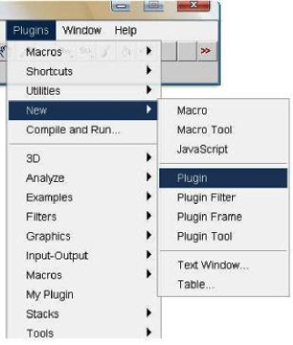
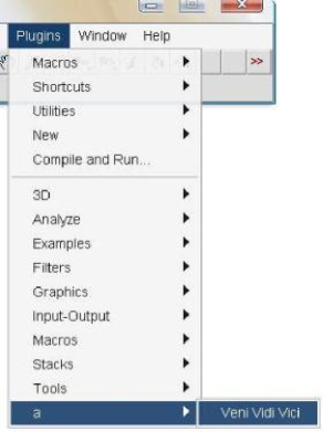
An editor pop ups to modify the run method. After compiling the plug-in, the created plug-in is shown in figure 4. Note that the name of the plug-in must contains underscores to be automatically loaded when ImageJ starts.

Figure 4: The created plug-in

5 Evaluation

To load an image, just drag-drop it on ImageJ. By clicking the menu item for the plug-in, it starts working.

Many trails were done to test the proposed framework. This was done on images provided on ImageJ site, shown in figure 5.

Figure 5: The original image

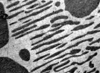
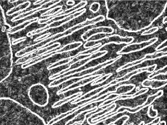
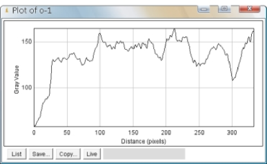
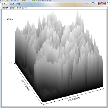
Many Veni operations can be done on the loaded image such as analysis plugins listed in section 3. Figures 6,7,8 shows the application of edge detection, plot profile, and surface plot.

Figure 6: edge detection

Figure 7: plot profile

Figure 8: surface plot

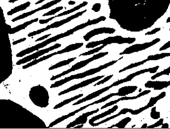
Many Vici operations can be done such as segmentation plugins listed in section 3. Figure 9 shows the application of Otsu thresholding technique [30]. This technique divides the histogram in two classes and then the inter-class variance is minimized. This plugin outputs a thresholded image with the selected threshold.

Figure 9: Otsu thresholding

6 Conclusion and Future Work

This paper proposes an alternative iterative approach to optimize input parameters and save time by minimizing the user involvement. This strategy is developed as custom plug-in in ImageJ.

The main focus was on developing an interactive visualization technique that enables users to analyze the relationships between sampled input parameters and corresponding output. This technique is implemented in a prototype called Veni Vidi Vici. It provides users with a visual overview of parameters and their sampled values. To find optimal parameter settings, users can select best possible configuration.

Not only the proposed framework facilitates better algorithm understanding, but also it can be used to explore the parameter space.

Future work have many dimension. One dimension is to consider the application of the proposed framework on temporal data such as feature point tracking and trajectory analysis for video imaging [31].

Another dimension is extending the theoretical foundation of the proposed framework to be able to answer some questions regarding the parameters of Veni, Vidi, and Vici. Questions such as : How does a slight parameter change modify the result? How stable is a parameter? In which range is a parameter stable?

Another dimension is to enhance the accuracy of the framework by incorporating transfer learning [32], to be able to generalize what learnt from one case to another. In many machine learning, there is an assumption that the training and future data must be in the same feature space and have the same distribution. However, in many real-world applications, this assumption may not hold. Knowledge transfer, if done successfully, would greatly improve the performance of learning by avoiding much expensive data-labeling efforts.

References

- [1] T. Walter, D. W. Shattuck, R. Baldock, M. E. Bastin, A. E. Carpenter, S. Duce, J. Ellenberg, A. Fraser, N. Hamilton, S. Pieper, M. A. Ragan, J. E. Schneider, P. Tomancak, and J.-K. H erich e. Visualization of image data from cells to organisms. NatureMethods Supplement, 7(3):S26 S41, 2010
- [2] A.J. Pretorius, M.-A.P. Bray, A.E. Carpenter and R.A. Ruddle, Visualization of parameter space for image analysis, IEEE Transactions on Visualization and Computer Graphics, vol. 17, no. 12, pp. 2402-2411, 2011.
- [3] Peter Sikachev and Artem Amirkhanov and Robert S. Laramee and Gabriel Mistelbauer. Interactive Algorithm Exploration using Meta Visualization, Technical report, Institute of Computer Graphics and Algorithms, Vienna University of Technology, 2011.
- [4] http://www.unrv.com/fall-republic/veni-vidi-vici.php.
- [5] N. J. Cutland. Computability: An Introduction to Recursive Function Theory, Cambridge University Press, 1980, pp. 72-84.
- [6] Collins TJ. ImageJ for microscopy. BioTechniques, 2007, volume 43, Suppl 1, pp.25 30.
- [7] L. Tweedie, B. Spence, H. Dawkes, and H. Su. The influence explorer. In Proceedings of the Conference on Human Factors in Computing Systems, pages 129 130, 1995.
- [8] L. Tweedie and R. Spence. The prosection matrix: a tool to support the interactive exploration of statistical models and data. Computational Statistics, 13(1):65 76, 1998.
- [9] K.-L. Ma. Image graphs a novel approach to visual data exploration. In Proceedings of the IEEE Conference on Visualization, pages 81 88, 1999.
- [10] L. Bavoil, S. P. Callahan, P. J. Crossno, J. Freire, and H. T. Vo. VisTrails: enabling interactive multiple-view visualizations. In Proceedings of the IEEE Conference on Visualization, pages 135 142, 2005.
- [11] S. P. Callahan, J. Freire, E. Santos, C. E. Scheidegger, C. T. Silva, and H. T. Vo. Managing the evolution of dataflows with VisTrails. In Proceedings of the International Conference on Data Engineering Workshops, pages 71 75, 2006.
- [12] T. J. Jankun-Kelly and K.-L.Ma. A spreadsheet interface for visualization exploration. In Proceedings of the IEEE Conference on Visualization, pages 69 76, 2000.
- [13] J. J. van Wijk and C. W. A. M. van Overveld. Preset based interaction with high dimensional parameter spaces. Data Visualization: The State of the Art, pages 391 406, 2003.
- [14] D. Foulser. IRIS Explorer: a framework for investigation. SIGGRAPH Computer Graphics, 29:13 16, 1995.
- [15] A. E. Carpenter, T. R. Jones, M. R. Lampbrecht, C. Clarke, I. H. Kang, O. Friman, D. A. Guertin, J. H. Chang, R. A. Lindquist, J. Moffat, P. Golland, and D.M. Sabatini. CellProfiler: image analysis software for identifying and quantifying cell phenotypes. Genome Biology, 7(R100), 2006.
- [16] Bruckner S., Gröller M. E. VolumeShop: An interactive system for direct volume illustration. In Proceedings of IEEE Visualization 2005 (October 2005), pp. 671 678.
- [17] Maryam Booshehrian, Torsten Möller, Randall M. Peterman, and Tamara Munzner. Vismon: Facilitating Risk Assessment and Decision Making In Fisheries Management, Technical report TR 2011-04, School of Computing Science, Simon Fraser University, Burnaby, BC, Canada, September 2011.
- [18] Maryam Booshehrian, Torsten Möller, Randall M. Peterman, and Tamara Munzner. Vismon: Facilitating Analysis of Trade-Offs, Uncertainty, and Sensitivity In Fisheries Management Decision Making, Computer Graphics Forum (Proceedings of Eurographics Conference on Visualization 2012 (EuroVis 2012)), vol. 31, no. 3, pp. 1235-1244.
- [19] Collie J. S., Peterman R. M., Zuelke B., A Risk Assessment Framework for AYK Salmon. Tech. rep., Project completion report for the Alaska Sustainable Salmon Fund, Nov. 2009.
- [20] Thomas Torsney-Weir, Ahmed Saad, Torsten Moller, Hans-Christian Hege, Britta Weber, and Jean-Marc Verbavatz. Tuner: Principled Parameter Finding for Image Segmentation Algorithms Using Visual Response Surface Exploration. IEEE Transactions on Visualization and Computer Graphics, volume 17, number 12, pp. 1892-1901, 2011.
- [21] http://www.cg.tuwien.ac.at/research/publications/2012/VisWeek-Tutorial-2012-Uncertainty/
- [22] Burger W, Burge M. Digital Image Processing: An Algorithmic Approach Using Java. Springer. ISBN 1-84628-379-5, 2007
- [23] Girish V, Vijayalakshmi A. Affordable image analysis using NIH Image/ImageJ. Indian J Cancer vol. 41, no. 1, pp. 47, 2004.
- [24] Eliceiri K, Rueden C. Tools for visualizing multidimensional images from living specimens. Photochem Photobiol vol. 81 , no. 5, pp. 1116 1122, 2005.
- [25] Barboriak D, Padua A, York G, Macfall J. Creation of DICOM Aware Applications Using ImageJ. J Digit Imaging , vol. 18, no. 2, pp. 91-99, 2005.
- [26] Rajwa B, McNally H, Varadharajan P, Sturgis J, Robinson J. AFM/CLSM data visualization and comparison using an open-source toolkit. Microsc Res Tech vol. 64, no. 2, pp. 176 184, 2004.
- [27] Gering E, Atkinson C. A rapid method for counting nucleated erythrocytes on stained blood smears by digital image analysis. J Parasitol vol. 90, no. 4, pp. 879 881, 2004.
- [28] Rueden CT, Eliceiri KW. Visualization approaches for multidimensional biological image data. BioTechniques vol. 43, Suppl. 1, pp. 33 36, 2007.
- [29] Davis, Martin D. Computability and Unsolvability. Dover Publishing, 1983
- [30] N. Otsu, A threshold selection method from gray level histograms, IEEE Trans. Systems, Man and Cybernetics, vol. 9, pp. 62-66 1979
- [31] I. F. Sbalzarini and P. Koumoutsakos. Feature Point Tracking and Trajectory Analysis for Video Imaging in Cell Biology, Journal of Structural Biology vol. 151, no. 2, pp. 182-195, 2005
- [32] Sinno Jialin Pan and Qiang Yang, A Survey on Transfer Learning, Knowledge and Data Engineering, IEEE Transactions on, 2010, volume 22, number 10, pages 1345-1359.