Approximation of high quantiles from intermediate quantiles

Abstract

Motivated by applications requiring quantile estimates for very small probabilities of exceedance $p_{n}\ll 1/n$, this article addresses estimation of high quantiles for $p_{n}$ satisfying $p_{n}\in[n^{-\tau_{2}},n^{-\tau_{1}}]$ for some $\tau_{1}>1$ and $\tau_{2}>\tau_{1}$. For this purpose, the tail regularity assumption $\log U\circ\exp\in ERV$ (with $U$ the left-continuous inverse of $1/(1-F)$, and $ERV$ the extended regularly varying functions) is explored as an alternative to the classical regularity assumption $U\in ERV$ (corresponding to the Generalised Pareto tail limit). Motivation for the alternative regularity assumption is provided, and it is shown to be equivalent to a limit relation for the logarithm of the survival function, the log-GW tail limit, which generalises the GW (Generalised Weibull) tail limit, a generalisation of the Weibull tail limit. The domain of attraction is described, and convergence results are presented for quantile approximation and for a simple quantile estimator based on the log-GW tail. Simulations are presented, and advantages and limitations of log-GW-based estimation of high quantiles are indicated.

Mathematics Subject Classification (2010): 60G70, 62G32, 26A12, 26A48

1 Introduction

An important application of extreme value theory is the estimation of tail quantiles. Theoretical analysis usually addresses tail quantile estimation from $n$ independent random variables $\{X_{1},...,,X_{n}\}$ with common distribution function $F$, and considers the asymptotic properties of estimators as $n\rightarrow\infty$. Of particular interest are high quantiles, exceeded with probabilities $p_{n}=O(1/n)$; see e.g. Weissman, (1978), Dekkers et al, (1989), de Haan & Rootz n, (1993) and for dependent random variables, Drees, (2003).

Let $X_{1,n}\leq X_{2,n}\leq...\leq X_{n,n}$ be the order statistics derived from $\{X_{1},...,,X_{n}\}$, and let $U$ denote the left-continuous inverse of $1/(1-F)$ on $(1,\infty)$. The intermediate quantile $U(n/k_{n})$, with the sequence $(k_{n})$ satisfying

$$k_{n}\in\{1,..,n\}\;\forall n\in\mathbb{N},\quad k_{n}/n\rightarrow 0\quad\textrm{and}\quad k_{n}\rightarrow\infty,$$ (1.1)

is under certain additional conditions estimated consistently by the intermediate order statistic $X_{n-k_{n}+1,n}$ (e.g. de Haan & Ferreira, (2006), Theorem 2.4.1). In contrast, the expected number of data points exceeding a high quantile is eventually bounded. A high quantile estimator can therefore not be expected to converge without some form of regularity of the tail, allowing it to be derived from intermediate order statistics.

The classical regularity assumption on the upper tail of the distribution function $F$ is often expressed as a condition on $U$; it requires that a positive function $w$ and a non-constant function $\varphi$ exist such that

$$\lim_{t\rightarrow\infty}\frac{U(t\lambda)-U(t)}{w(t)}=\varphi(\lambda)\quad\forall\lambda\in C_{\varphi},$$ (1.2)

with $C_{\varphi}$ the continuity points of $\varphi$ in $(0,\infty)$. As the limiting function $\varphi$ is continuous (e.g. de Haan & Ferreira, (2006), Theorem 1.1.3), $U$ satisfying (1.2) is extended regularly varying (see e.g. Appendix B2 of de Haan & Ferreira, (2006), or Chapter 3 of Bingham et al, (1987)). Therefore, $w$ can be chosen to be regularly varying and (since $U$ is nondecreasing) such that

$$\varphi=h_{\gamma}$$ (1.3)

for some real $\gamma$ with for all positive $\lambda$,

$$h_{\gamma}(\lambda):={\scriptstyle\int_{1}^{\lambda}}t^{\gamma-1}dt,$$ (1.4)

which is $\gamma^{-1}(\lambda^{\gamma}-1)$ if $\gamma\neq 0$ and $\log\lambda$ if $\gamma=0$; (1.2) with (1.3) is equivalent to a Generalised Pareto (GP) tail limit for the survival function (e.g. de Haan & Ferreira, (2006), Theorem 1.1.2). In (1.2), the limit on the right-hand side was left unspecified in order to stress the nonparametric nature of the classical regularity assumption, which makes it particularly attractive from the point of view of applications.

When referring to (1.2), we will write $U\in ERV$, with $ERV$ the extended regularly varying functions. We will write $U\in ERV_{S}$ to specify that in addition, (1.3) holds with $\gamma\in S\subset\mathbb{R}$, and $U\in ERV_{\{\gamma\}}(w)$ for (1.2) and (1.3) with a particular $\gamma$ and positive $w$. We will apply the same notational conventions when a limit relation of the form (1.2) applies to a nondecreasing function other than $U$. For a regularly varying function $g$ (e.g. Bingham et al, (1987)), we will write $g\in RV$, or $g\in RV_{S}$ to specify that $\lim_{t\rightarrow\infty}g(t\lambda)/g(t)=\lambda^{\alpha}$ for all $\lambda>0$ for some $\alpha\in S\subset\mathbb{R}$.

It has been known for long that existence of the limit (1.2) alone is of limited value for approximation of a high quantile $U(1/p_{n})$ with $p_{n}=O(1/n)$ from an intermediate quantile $U(n/k_{n})$ with $(k_{n})$ as in (1.1), since $\lambda_{n}:=k_{n}/(np_{n})\rightarrow\infty$ as $n\rightarrow\infty$. Usually, additional assumptions on the rate of convergence in (1.2) are introduced for this purpose, such as (strong) second-order extended regular variation (de Haan & Stadtm ller, (1996), de Haan & Ferreira, (2006)), the Hall class (Hall, (1982)), or conditions (1.5) and (1.6) of de Haan & Rootz n, (1993).

In this article, a different approach is explored: instead of strengthening (1.2), we will look for an alternative regularity assumption specifically to approximate certain high quantiles from intermediate quantiles, and by extension, to estimate such high quantiles. The quantiles we will focus on are very high quantiles corresponding to probabilities of exceedance $(p_{n})$ satisfying

$$p_{n}\in[n^{-\tau_{2}},n^{-\tau_{1}}]\quad\textrm{for some}\quad\tau_{1}>1,\;\tau_{2}>\tau_{1},$$ (1.5)

without excluding that the approximation may also be suitable for less rapidly vanishing $(p_{n})$. This choice is motivated by applications requiring quantile estimates for probabilities of exceedance $p_{n}$ satisfying $p_{n}n\ll 1$, such as flood hazard assessment (de Haan, (1990)), design criteria on wind, waves and currents for offshore structures (ISO, (2005), paragraph A.5.7), seismic hazard assessment (Adams & Atkinson, (2003)) and analysis of bank operational risk (Cope et al, (2009)). In such applications, one would want an estimator for $U(1/p_{n})$ which converges in a meaningful sense even when $p_{n}n\rightarrow 0$ as $n\rightarrow\infty$. However, the latter condition is difficult to handle in its full generality. Therefore, we will narrow the focus to $(p_{n})$ satisfying (1.5). Moreover, we will try to find an estimator which for $p_{n}=n^{-\tau}$ converges (in some yet-to-be-defined sense) uniformly in $\tau\in[1,T]$ for every $T>1$. In practical terms, this means that if the assumptions for convergence are satisfied, then an estimate of a quantile exceeded with a probability of, say, 0.01 can be extended to an estimate of the quantile exceeded with a probability of 0.0001 without seriously stretching the assumptions, as these probabilities differ only a factor of two in terms of $\tau$. Such flexibility is important in applications, because $p_{n}$ is generally based on social and economic considerations, without regard for the feasibility of estimating $U(1/p_{n})$.

For convenience, we will assume throughout that $U(\infty):=\lim_{t\rightarrow\infty}U(t)>1$.

2 An alternative regularity condition

The alternative regularity assumption on the upper tail of $F$ proposed for estimation of a very high quantile $U(1/p_{n})$ with $(p_{n})$ satisfying (1.5) is

$$\log q\in ERV$$ (2.1)

with

$$q:=U\circ\exp.$$ (2.2)

(2.1) is of the same nonparametric form as the classical regularity assumption (1.2), but with $U$ replaced by $\log U\circ\exp$. Therefore, it implies that for some real $\theta$ and positive function $g$,

$$\lim_{y\rightarrow\infty}\frac{\log q(y\lambda)-\log q(y)}{g(y)}=h_{\theta}(\lambda)\quad\forall\lambda>0.$$ (2.3)

To see the relevance of (2.1) for approximation of a very high quantile $q(-\log p_{n})=U(1/p_{n})$ with $(p_{n})$ satisfying (1.5) from an intermediate quantile $q(\log(n/k_{n}))=U(n/k_{n})$, assume that in addition to (1.1), $\limsup_{n\rightarrow\infty}\log k_{n}/\log n<1.$ This ensures that $-\log p_{n}=O(\log(n/k_{n}))$ as $n\rightarrow\infty$, and since convergence in (2.3) is locally uniform in $\lambda>0$ (e.g. Bingham et al, (1987), Theorem 3.1.16), it implies

$$\lim_{n\rightarrow\infty}\left|\frac{\log U(1/p_{n})-\log U(n/k_{n})}{g(\log(n/k_{n}))}-h_{\theta}\left(\frac{\log(1/p_{n})}{\log(n/k_{n})}\right)\right|=0.$$

The limit relation (2.3) can be reformulated in terms of the survival function:

Theorem 2.1

The limit relation (2.3) for some positive function $g$ and real $\theta$ is equivalent to

$$\lim_{y\rightarrow\infty}\frac{\log(1-F(q(y)\textrm{e}^{xg(y)}))}{y}=-h_{\theta}^{-1}(x)\quad\forall x\in h_{\theta}(\mathbb{R}^{+}),$$ (2.4)

Proof

Equivalence of (2.3) and (2.4) is implied by Lemma 1.1.1 in de Haan & Ferreira, (2006). ∎

The pair (2.3) and (2.4) of equivalent limits can be seen as the analogue for $\log q$ of (1.2) with $\varphi=h_{\gamma}$ and the equivalent GP limit for the survival function

$$\lim_{t\rightarrow\infty}t(1-F(xw(t)+U(t)))=1/h_{\gamma}^{-1}(x)\quad\forall x\in h_{\gamma}(\mathbb{R}^{+})$$ (2.5)

(e.g. de Haan & Ferreira, (2006), Theorem 1.1.2). It is important to realise that convergence of a log-ratio of probabilities as in (2.4) is a much weaker notion than convergence of a ratio of probabilities as in the GP limit (2.5). This difference reflects precisely the difference in extrapolation range between (2.3) and (1.2): when extrapolating over a longer range, larger errors should be expected in principle, unless additional assumptions apply.

To illustrate that condition (2.1) is a natural assumption, Proposition 1 below shows how it may arise in the context of a GP tail limit (1.2) with (1.3) and the GP quantile approximation

$$\tilde{U}_{t}(z):=U(t)+h_{\gamma}(z/t)w(t)$$ (2.6)

with $w$ and $\gamma$ as in (1.2) and (1.3).

Proposition 1

Let $U\in ERV_{\{\gamma\}}(w)$.

(a) If $\gamma>0$, then

$$\lim_{t\rightarrow\infty}\frac{\log\tilde{U}_{t}(t^{\lambda})-\log U(t^{\lambda})}{\log U(t^{\lambda})-\log U(t)}=0\quad\forall\lambda>1$$ (2.7)

and

$$\log q\in ERV_{\{1\}}.$$

(b) If $\gamma=0$ and

$$\lim_{t\rightarrow\infty}\frac{\tilde{U}_{t}(t^{\lambda})-U(t^{\lambda})}{U(t^{\lambda})-U(t)}=0\quad\forall\lambda>1,$$ (2.8)

then

$$q\in ERV_{\{1\}}\quad\textrm{and}\quad\log q\in ERV_{\{0\}}(1).$$

Proof

The proof is found in Subsection 7.1.

For distribution functions in the domain of attraction of the GP tail limit, Proposition 1 shows that the condition (2.1) must hold if $\gamma>0$; if $\gamma=0$, it is a necessary condition for convergence of the relative error in the GP approximation in the sense of (2.8).

Proposition 1 also provides some basic insight into the strengths and limitations of the GP quantile approximation (2.6) for very high quantiles. If $\gamma>0$, there is no problem; the notion of convergence in (2.7) may be weak, but can be considered appropriate for these heavy-tailed distribution functions. However, if $\gamma=0$ and (2.8) holds, then necessarily, $q\in ERV_{\{1\}}$, which is a restrictive condition. For example, for the normal distribution, $q\in ERV_{\{1/2\}}$, so (2.8) cannot hold.

In analogy to (1.2), a natural generalisation of $q\in ERV_{\{1\}}$ would be $q\in ERV$, so for some real $\theta$ and some positive function $g$,

$$\lim_{y\rightarrow\infty}\frac{q(y\lambda)-q(y)}{g(y)}=h_{\theta}(\lambda)\quad\forall\lambda>0.$$ (2.9)

By a slight modification of Theorem 2.1, (2.9) is equivalent to

$$\lim_{y\rightarrow\infty}\frac{\log(1-F(xg(y)+q(y)))}{y}=-h_{\theta}^{-1}(x)\quad\forall x\in h_{\theta}(\mathbb{R}^{+}).$$ (2.10)

Furthermore, if $\theta>0$, then $q\in RV_{\{\theta\}}$ (de Haan & Ferreira, (2006), Theorem B.2.2(1)) and we may take $\theta q$ for $g$ in (2.10), resulting in

$$\lim_{y\rightarrow\infty}\frac{\log(1-F(xq(y)))}{y}=-x^{1/\theta}\quad\forall x>0.$$ (2.11)

The equivalent limit relations $q\in RV_{\{\theta\}}$ and (2.11) with $\theta>0$ are known as the Weibull tail limit; see e.g. Broniatowski, (1993), Kl ppelberg, (1991), Gardes et al, (2011) and references in the latter. Therefore, we will refer to both (2.9) and (2.10) as the Generalised Weibull (GW) tail limit. Among the distribution functions with a GW tail limit are the Weibull, gamma, and normal distributions, but also lighter-tailed distribution functions satisfying $q\in ERV_{(-\infty,0]}$. The latter satisfy $\lim_{y\rightarrow\infty}q(y\xi)/q(y)=1$ for all $\xi>1$; if $q\in ERV_{(-\infty,0)}$, then $q(\infty)$ is finite.

In view of the above, we will refer to (2.3) and (2.4) as the log-GW tail limit. Just as $q\in ERV$ generalises the condition $q\in ERV_{\{1\}}$ arising in the context of a GP limit and GP quantile approximation in Proposition 1(b), we can see $\log q\in ERV$ as a natural generalisation of the restrictive conditions $\log q\in ERV_{\{1\}}$ and $\log q\in ERV_{\{0\}}(1)$ in Proposition 1(a) and (b), respectively. Furthermore, the log-GW tail limit generalises the GW tail limit: if $F$ satisfies $q\in ERV_{\{\theta\}}$, then it must also satisfy $\log q\in ERV_{\{\min(\theta,0)\}}$; see e.g. Dekkers et al, (1989) (Lemma 2.5) and Lemma 1(a) in Subsection 7.9, included for convenience. Therefore, the log-GW tail limit is the more important limit relation to consider as regularity assumption. Nevertheless, the GW limit may be useful in certain applications involving distribution functions with moderate or light tails. In particular, if $\theta<0$, then $\log q\in ERV_{\{\theta\}}$ if and only if $q\in ERV_{\{\theta\}}$; see Lemma 1(c) in Subsection 7.9.

The following result supplements Proposition 1 by describing the possible overlap of the domain of attraction of the GP limit with the domains of attraction of the GW and log-GW limits. It just states the plain results; an interpretation follows.

Theorem 2.2

For $q:=U\circ\exp$,

• If $U\in ERV$ and $q\in ERV$, then $U\in ERV_{\{0\}}$.

• If $U\in ERV$ and $\log q\in ERV$, then

  • (i) $U\in ERV_{\{0\}}\;and\;\log q\in ERV_{(-\infty,1]},$

  • (ii) $U\in ERV_{(0,\infty)}\;and\;\log q\in ERV{}_{\{1\}}.$

Proof

See Subsection 7.2.

Theorem 2.2(a) supplements Proposition 1(b) for the $\gamma=0$ case: the existence of a GW limit excludes distribution functions with heavy and light GP tail limits. Theorem 2.2(b) identifies which specific log-GW limits may coexist with a GP limit. Case (ii) is the classical Pareto limit encountered in Proposition 1(a). Case (i) concerns lighter tails; note that it is possible that $U\in ERV_{\{0\}}$ and $\log q\in ERV_{\{1\}}$, an example being $q(y)=\exp(y/\log(y+1)-1)$. By assertion (b), a GP limit with $\gamma<0$ excludes a log-GW limit.

The domain of attraction of the log-GW limit covers a wide range of tail behaviour. It includes the domain of attraction of the GW limit described earlier, and the domain of attraction of the Pareto limit with $\gamma>0$, but also the distribution functions satisfying $\log q\in ERV_{(0,1)}$, with tails heavier than a Weibull tail but lighter than a Pareto tail. As such, it achieves a “unification” of the Pareto and Weibull tail limits sought in Gardes et al, (2011). An example is the lognormal distribution, which satisfies $\log q\in ERV_{\{\nicefrac{{1}}{{2}}\}}$; neither (2.8), nor (2.7) holds for this distribution function. Finally, the domain of attraction of the log-GW limit also includes the very heavy-tailed distribution functions satisfying $\log q\in ERV_{(1,\infty)}$, which do not have classical limits. For these, the mean of the excess $(X-\alpha)\vee 0$ over any finite threshold $\alpha$ is infinite.

Having now established the log-GW limit as a widely applicable regularity assumption for approximation of high quantiles with probabilities $(p_{n})$ satisfying (1.5), the following sections will address the use of a log-GW tail as model for quantile approximation and estimation.

3 Approximation and convergence

The log-GW limit suggests to approximate a quantile $q(z)$ for $z>0$ by $q(y)\textrm{e}^{g(y)h_{\theta}(z/y)}$ for $y\in q^{-1}((0,\infty))$ and with $g$ and $\theta$ as in (2.3). As an introduction to the quantile estimator presented in the next section, we will consider the following somewhat more general log-GW quantile approximation:

$$\tilde{q}_{y}(z):=q(y)\textrm{e}^{\tilde{g}(y)h_{\tilde{\theta}(y)}(z/y)},$$ (3.1)

with $\tilde{\theta}$ a real function and $\tilde{g}$ a positive function, related to $q$ as follows: for some $\xi>1$,

$$\tilde{\theta}(y)-a_{\xi}(y)\rightarrow 0\quad\textrm{and}\quad\tilde{g}(y)\sim(\log q(y\xi)-\log q(y))/h_{\tilde{\theta}(y)}(\xi)\quad\textrm{as}\;y\rightarrow\infty$$ (3.2)

with for every $\iota\in(0,1)\cup(1,\infty)$,

$$a_{\iota}(y):=\frac{\log\left|\log q(y\iota^{2})-\log q(y\iota)\right|-\log\left|\log q(y\iota)-\log q(y)\right|}{\log\iota}.$$ (3.3)

If $q$ has a second derivative $q^{\prime\prime}$, then $a_{\iota}(y)$ may be regarded as a finite-difference approximation of $y(\log(y(\log q(y))^{\prime}))^{\prime}=1+yq^{\prime\prime}(y)/q^{\prime}(y)-yq^{\prime}(y)/q(y)$, a scale-invariant measure of curvature.

If $\log q\in ERV_{\{\theta\}}(g)$, then $\log q(\textrm{Id}\cdot\xi)-\log q\in RV_{\{\theta\}}$ for every $\xi>1$ and (3.2) is equivalent to $\tilde{\theta}(y)\rightarrow\theta$ and $\tilde{g}(y)\sim g(y)$ as $y\rightarrow\infty$. The following is a straightforward consequence:

Proposition 2

If $\log q\in ERV_{\{\theta\}}(g)$ and the real function $\tilde{\theta}$ and positive function $\tilde{g}$ satisfy (3.2), then $\tilde{q}_{y}$ defined by (3.1) satisfies

$$\lim_{y\rightarrow\infty}\sup_{\lambda\in[\Lambda^{-1},\Lambda]}\left|\frac{\log\tilde{q}_{y}(y\lambda)-\log q(y\lambda)}{g(y)}\right|=0\quad\forall\Lambda>1,$$ (3.4)

and if

$$\limsup_{y\rightarrow\infty}g(y)<\infty$$ (3.5)

(for example, if $q\in ERV$), then in addition,

$$\lim_{y\rightarrow\infty}\sup_{\lambda\in[\Lambda^{-1},\Lambda]}\left|\frac{\tilde{q}_{y}(y\lambda)-q(y\lambda)}{q(y)g(y)}\right|=0\quad\forall\Lambda>1.$$ (3.6)

Proof

A proof of this standard result can be found in Subsection 7.3.

Remark 1

Eq. (3.4) remains valid when $g(y)$ in the denominator is replaced by $\log q(y)$ or by $\log q(y\xi)-\log q(y)$ for any $\xi\in(0,\infty)\setminus\{1\}$, because by (2.3),

$$g(y)/\bigl{|}\log q(y\xi)-\log q(y)\bigr{|}=O(1)$$ (3.7)

as $y\rightarrow\infty$, and therefore also $g(y)/\log q(y)=O(1)$.

Condition (3.5) implies that $\theta\leq 0$ in (2.3) and therefore, that $q$ is of bounded increase (see Bingham et al, (1987), Section 2.1); vice versa, bounded increase of $q$ implies (3.5) by (2.3). If (3.5) holds, then (3.4) and (3.6) remain valid when $g(y)$ is replaced by $1$. Furthermore, $q(y)g(y)$ in (3.6) can be replaced by $q(y\xi)-q(y)$ for any $\xi\in(0,\infty)\setminus\{1\}$; see Subsection 7.4. Furthermore, if $q(\infty)<\infty$, then we may also replace $q(y)g(y)$ in (3.6) by $q(\infty)-q(y\eta)$ for any $\eta>0$; see Subsection 7.4.

The normalisation of the quantile approximation error in (3.4) is model-dependent. Whether (3.6) is applicable, and which model-independent normalisations may be substituted for $g$ in (3.4) and (3.6), depends on tail weight: i.e., on whether $q$ is of bounded increase; see Remark 1. As an alternative, the error in a quantile approximation may be expressed in terms of a mismatch between the probabilities of exceedance of the quantile and of its approximation. As we will see shortly, this can be done in such a way that a single model-independent notion of convergence holds if $\log q\in ERV$.

There may also be other reasons for considering probability-based quantile approximation and estimation errors. For example, in the context of structural reliability analysis and safety engineering (e.g. flood protection, tall buildings, bridges, offshore structures, etc.), the required overall safety level constrains a design; usually, it takes the form of a maximum tolerated failure rate, fixed in legislation or in rules issued by regulators or classification societies. Within this context, errors in estimates of load quantiles are often viewed in terms of equivalent errors in frequency of exceedance.

In the present context, a natural expression of the mismatch between $1-F(\tilde{q}_{y}(z))$ and $1-F(q(z))$ is

$$\tilde{\nu}_{y}(z):=\frac{q^{-1}(\tilde{q}_{y}(z))}{q^{-1}(q(z))}-1=\frac{\log(1-F(\tilde{q}_{y}(z)))}{\log(1-F(q(z)))}-1.$$ (3.8)

Because $F$ may be constant over some interval, it is possible that $\tilde{\nu}_{y}(z)=0$ while $\tilde{q}_{y}(z)>q(z)$. If $q(\infty)<\infty$ and $\tilde{q}_{y}(z)>q(\infty)$, then $\tilde{\nu}_{y}(z)=\infty$. If $F$ is continuous, then $-\log(1-F(q(z)))=q^{-1}(q(z))=z$ in (3.8).

For the log-GW approximation (3.1), convergence of $\tilde{\nu}_{y}(y\lambda)$ to zero as $y\rightarrow\infty$ for $\lambda>0$ is a similarly weak notion of convergence as convergence to the log-GW limit in (2.4). In fact, if $F$ is continuous, then with $\tilde{\theta}(y)=\theta$ and $\tilde{g}(y)=g(y)$ in (3.1), the log-GW limit can be written alternatively as $\lim_{y\rightarrow\infty}\lambda\tilde{\nu}_{y}(y\lambda)=0$ for all $\lambda>0$. A somewhat more general result is the following.

Theorem 3.1

If $\log q\in ERV$ and real functions $\tilde{\theta}$ and $\tilde{g}$, $\tilde{g}$ positive, satisfy (3.2), then $\tilde{q}_{y}$ defined by (3.1) satisfies

$$\lim_{y\rightarrow\infty}\sup_{\lambda\in[\Lambda^{-1},\Lambda]}\left|\tilde{\nu}_{y}(y\lambda)\right|=0\quad\forall\Lambda>1.$$ (3.9)

Proof

See Subsection 7.5.

Alternatively, one may want to consider a stronger notion of convergence such as

$$\lim_{y\rightarrow\infty}\frac{1-F(q(y\lambda))}{1-F(\tilde{q}_{y}(y\lambda))}=1\qquad\forall\lambda\geq 1.$$ (3.10)

If $\lim_{y\rightarrow\infty}y^{-1}\log(1-F(q(y)))=-1$, then by taking the logarithm, (3.10) can be seen to be equivalent to $\lim_{y\rightarrow\infty}y\tilde{\nu}_{y}(y\lambda)=0$ for all $\lambda\geq 1$. Ensuring this convergence rate condition requires strengthening of the assumption of a log-GW limit. We will discuss this further within the context of a specific estimator in the next section.

4 A simple high quantile estimator

To demonstrate the potential of the alternative regularity condition for estimation of high quantiles, this section introduces a quantile estimator closely related to the log-GW approximation (3.1) and presents consistency results.

Consider a sequence of independent random variables $(X_{n})$ with $X_{i}\sim F$ for all $i\in\mathbb{N}$. Let $X_{k,n}$ denote the $k$-th lowest order statistic out of $\{X_{1},..,X_{n}\}$. Let $\iota>1$ be fixed, and let $k_{2}:\mathbb{\mathbb{N}\rightarrow N}$ be nondecreasing and such that $k_{2}(n)\in\{1,...,n-1\}$ for all $n\in\mathbb{N}$. Define for $j\in\{0,1\}$,

$$k_{j}(n):=\left\lfloor(k_{2}(n)/n)^{\iota^{j-2}}n\right\rfloor.$$ (4.1)

A simple log-GW-based estimator for a quantile $q(z)$ with probability of exceedance $\textrm{e}^{-z}$ is $\hat{q}_{n}(z)$, defined for every $z>0$ and $n\in\mathbb{N}$ such that $X_{n-k_{0}(n)+1,n}>0$ by

$$\hat{q}_{n}(z):=X_{n-k_{0}(n)+1,n}\exp\left(\hat{g}_{n}h_{\hat{\theta}_{n}}(z/y_{n})\right)$$ (4.2)

with

$$\hat{\theta}_{n}:=\frac{\log\log\frac{X_{n-k_{2}(n)+1,n}}{X_{n-k_{1}(n)+1,n}}-\log\log\frac{X_{n-k_{1}(n)+1,n}}{X_{n-k_{0}(n)+1,n}}}{\log\iota},$$ (4.3)

$$\hat{g}_{n}:=\frac{\log\frac{X_{n-k_{1}(n)+1,n}}{X_{n-k_{0}(n)+1,n}}}{h_{\hat{\theta}_{n,\iota}}(\iota)},$$ (4.4)

and

$$y_{n}:=\log(n/k_{0}(n)).$$ (4.5)

This estimator can be regarded as a straightforward application of the approximation (3.1) to the sampling distribution of $\{X_{1},..,X_{n}\}$ instead of $F$, taking

$$g_{\iota}(y):=(\log q(y\iota)-\log q(y))/h_{a_{\iota}(y)}(\iota)$$ (4.6)

for $\tilde{g}(y)$ and $a_{\iota}(y)$ for $\tilde{\theta}(y)$. Assume that $k_{2}(n)/n\rightarrow 0$ and $k_{2}(n)\rightarrow\infty$ as $n\rightarrow\infty$. Then by (4.1), as $\iota>1$, also $k_{j}(n)/n\rightarrow 0$ and $k_{j}(n)\rightarrow\infty$ as $n\rightarrow\infty$ for $j=1$ and $j=0$. Moreover, if $k_{2}$ is chosen to satisfy

$$\limsup_{n\rightarrow\infty}\frac{\log k_{2}(n)}{\log n}=:c<1,$$ (4.7)

then by (4.1), $\limsup_{n\rightarrow\infty}(\log k_{0}(n))/\log n=1+\iota^{-2}(c-1)$, so

$$\liminf_{n\rightarrow\infty}y_{n}/\log n=(1-c)\iota^{-2}.$$ (4.8)

Therefore, for every $T\geq 1$, eventually

$$[T^{-1}\log n,T\log n]\subset[\lambda^{-1}y_{n},\lambda y_{n}]\quad\forall\lambda>T\iota^{2}/(1-c),$$ (4.9)

and as a result, $-\log p_{n}$ with $(p_{n})$ as in (1.5) is eventually in the interval $[\lambda^{-1}y_{n},\lambda y_{n}]$ for some $\lambda>1$.

If $\log X$ were replaced by $X$ in (4.2)-(4.4) and (4.1) were modified to $k_{j}(n):={\scriptstyle\left\lfloor k_{2}(n)\iota^{2-j}\right\rfloor}$ and (4.5) to $y_{n}:=n/k_{0}(n)$, then with $\iota=2$, (4.3) would become the Pickands, (1975) estimator for the extreme value index $\gamma$, and (4.2) would become an estimator for $U(z)$. Pickands’ estimator is known to be inaccurate in comparison to other commonly used estimators; see e.g. de Haan & Ferreira, (2006). The estimator $\hat{q}_{n}$, also based on only three order statistics, was chosen as an example here because of its simplicity.

Analogous to $\tilde{\nu}_{y}(z)$ in (3.8), define the probability-based quantile estimation error

$$\hat{\nu}_{n}(z):=\frac{q^{-1}(\hat{q}_{n}(z))}{q^{-1}(q(z))}-1=\frac{\log(1-F(\hat{q}_{n}(z)))}{\log(1-F(q(z)))}-1.$$ (4.10)

Theorem 4.1

Let $k_{2}:\mathbb{\mathbb{N}\rightarrow N}$ satisfy (4.7) and $k_{2}(n)/\log\log n\rightarrow\infty$ as $n\rightarrow\infty$. Consider $\hat{q}_{n}$, $\hat{\theta}_{n}$ and $\hat{g}_{n}$ defined by (4.1)-(4.5) for some $\iota>1$. If $\log q\in ERV_{\{\theta\}}(g)$, then

$$\hat{\theta}_{n}\rightarrow\theta\quad and\quad\hat{g}_{n}/g(y_{n})\rightarrow 1\quad a.s.$$ (4.11)

and for every $T>1$ (see (3.8)),

$$\sup_{\tau\in[T^{-1},T]}\left|\hat{\nu}_{n}(\tau\log n)\right|\rightarrow 0\quad\textrm{a.s.},$$ (4.12)

$$\sup_{\tau\in[T^{-1},T]}\left|\frac{\log\hat{q}_{n}(\tau\log n)-\log q(\tau\log n)}{g(y_{n})}\right|\rightarrow 0\quad a.s.$$ (4.13)

and if (3.5) holds (for example, if $q\in ERV$), then in addition,

$$\sup_{\tau\in[T^{-1},T]}\left|\frac{\hat{q}_{n}(\tau\log n)-q(\tau\log n)}{q(y_{n})g(y_{n})}\right|\rightarrow 0\quad a.s.$$ (4.14)

Proof

The proof is found in Subsection 7.6.

Theorem 4.1 establishes almost sure convergence of very high quantile estimates for probabilities of exceedance of $n^{-\tau}$ uniformly for all $\tau$ in an arbitrary compact subset of $(0,\infty)$ if $\log q\in ERV$.

Remark 2

Remark 1 about the normalisation in (3.4) and (3.6) carries over to (4.13) and (4.14).

For the analysis of the asymptotic distributions of errors, the assumption $\log q\in ERV_{\{\theta\}}$ in Theorem 4.1 will be strengthened somewhat. We assume that the derivative $q^{\prime}$ of $q$ exists, and

$$(\log q)^{\prime}=q^{\prime}/q\in RV_{\{\theta-1\}},$$ (4.15)

which implies $\log q\in ERV_{\{\theta\}}(\bar{g})$ with

$$\bar{g}(y)=yq^{\prime}(y)/q(y).$$ (4.16)

If it is given that $\log q\in ERV_{\{\theta\}}$ and that $q$ is differentiable, several seemingly weak conditions on $q^{\prime}$ are known which ensure (4.15); see e.g. Bingham et al, (1987) (Theorems 1.7.5 and 3.6.10).

Let $g_{\iota}$ be defined by (4.6), $a_{\iota}$ be defined by (3.3), and let

$$\kappa_{\theta}(\lambda,\iota):=\frac{\partial(h_{\theta}(\lambda)/h_{\theta}(\iota))}{\partial\theta}=\begin{cases}\frac{1}{\iota^{\theta}-1}\left(\lambda^{\theta}\log\lambda-\frac{\lambda^{\theta}-1}{\iota^{\theta}-1}\iota^{\theta}\log\iota\right)&\textrm{if\>}\theta\neq 0\\ \frac{1}{2}\log\lambda\left(\frac{\log\lambda}{\log\iota}-1\right)&\textrm{if\>}\theta=0\end{cases}$$ (4.17)

for all real $\theta$, $\iota\in(0,1)\cup(1,\infty)$ and $\lambda>0$; note that $\kappa_{\theta}(1,\iota)=\kappa_{\theta}(\iota,\iota)=0$. We will first consider limiting distribution functions of suitably normalised deviations of the estimates $\hat{\theta}_{n}$, $\hat{q}_{n}$ and $\hat{\nu}_{n}$ from their deterministic analogues.

Theorem 4.2

If (4.15) holds in addition to the assumptions for Theorem 4.1, then

$$Z_{n}:=\bigl{(}\hat{\theta}_{n}-a_{\iota}(y_{n})\bigr{)}y_{n}\sqrt{k_{2}(n)}h_{\theta}(\iota)\overset{d}{\rightarrow}N(0,(\iota^{\theta-2}/\log\iota)^{2})$$ (4.18)

and with $\tilde{\theta}=a_{\iota}$ and $\tilde{g}=g_{\iota}$ in (3.1), for all $T>1$,

$$\sup_{z\in[T^{-1}\log n,T\log n]}\left|\bigl{(}\hat{\nu}_{n}(z)-\tilde{\nu}_{y_{n}}(z)\bigr{)}y_{n}\sqrt{k_{2}(n)}-\Bigl{(}\frac{z}{y_{n}}\Bigr{)}^{-\theta}\kappa_{\theta}\Bigl{(}\frac{z}{y_{n}},\iota\Bigr{)}Z_{n}\right|\rightarrow 0\quad a.s.$$ (4.19)

and

$$\sup_{z\in[T^{-1}\log n,T\log n]}\left|\frac{\log\hat{q}_{n}(z)-\log\tilde{q}_{y_{n}}(z)}{g(y_{n})}y_{n}\sqrt{k_{2}(n)}-\kappa_{\theta}\Bigl{(}\frac{z}{y_{n}},\iota\Bigr{)}Z_{n}\right|\rightarrow 0\quad a.s.$$ (4.20)

for every positive function $g$ satisfying (2.3).

Proof

See Subsection 7.7.

Under an additional convergence rate assumption, the previous result implies asymptotic normality of the estimation errors $\hat{\theta}_{n}-\theta$, $\hat{\nu}_{n}$ and $\log\hat{q}_{n}-\log q$:

Corollary 1

If in addition to the assumptions for Theorem 4.2, (4.15) is strengthened to

$$\frac{q^{\prime}(y\lambda)/q(y\lambda)}{q^{\prime}(y)/q(y)}=\lambda^{\theta-1}(1+o(1)/\phi(y))\quad as\quad y\rightarrow\infty\quad\forall\lambda>1$$ (4.21)

with $\phi$ some positive increasing function satisfying $\lim_{y\rightarrow\infty}\phi(y)/(y\sqrt{\log y})=\infty$, and if $k_{2}$ satisfies $k_{2}(n)=O(\phi^{2}(y_{n})y_{n}^{-2})$, then

$$Z_{n}^{0}:=\bigl{(}\hat{\theta}_{n}-\theta\bigr{)}y_{n}\sqrt{k_{2}(n)}h_{\theta}(\iota)\overset{d}{\rightarrow}N(0,(\iota^{\theta-2}/\log\iota)^{2}),$$ (4.22)

and for all $T>1$,

$$\sup_{z\in[y_{n},T\log n]}\left|\hat{\nu}_{n}(z)\>y_{n}\sqrt{k_{2}(n)}-\Bigl{(}\frac{z}{y_{n}}\Bigr{)}^{-\theta}\kappa_{\theta}\Bigl{(}\frac{z}{y_{n}},\iota\Bigr{)}Z_{n}^{0}\right|\rightarrow 0\quad a.s.$$ (4.23)

and

$$\sup_{z\in[y_{n},T\log n]}\left|\frac{\log\hat{q}_{n}(z)-\log q(z)}{g(y_{n})}y_{n}\sqrt{k_{2}(n)}-\kappa_{\theta}\Bigl{(}\frac{z}{y_{n}},\iota\Bigr{)}Z_{n}^{0}\right|\rightarrow 0\quad a.s.$$ (4.24)

for every positive function $g$ satisfying (2.3).

Proof

See Subsection 7.7.

Remark 3

Eq. (4.19) and (4.7) imply that $y_{n}\sqrt{k_{2}(n)}(\hat{\nu}_{n}(y_{n}\lambda)-\tilde{\nu}_{y_{n}}(y_{n}\lambda))$ is asymptotically normal with zero mean and variance equal to $((\iota^{\theta-2}/\log\iota)\lambda^{-\theta}\kappa_{\theta}\left(\lambda,\iota)\right)^{2}$ for every $\lambda>0$. Similar comments apply to (4.20), (4.23) and (4.24).

Remark 4

If a function $\phi$ satisfying the conditions of Corollary 1 exists, then a $k_{2}$ satisfying $k_{2}(n)=O(\phi^{2}(y_{n})y_{n}^{-2})$, $k_{2}(n)/\log\log n\rightarrow\infty$ as $n\rightarrow\infty$ and (4.7) can always be found; for example, for some $\alpha>0$, one can take for $k_{2}(n)$ the smallest integer $k$ satisfying $k\geq\max(1,{\scriptstyle\left\lfloor\min(\textrm{e}^{\alpha y},\phi^{2}(y)y^{-2})\right\rfloor})$ with $y=\iota^{-2}\log(n/k)$.

Remark 5

Using (4.10), it can be seen that (4.23) implies

$$\sup_{z\in[y_{n},T\log n]}\biggl{|}\frac{1-F(q(z))}{1-F(\hat{q}_{n}(z))}-1\biggr{|}\overset{p}{\rightarrow}0\qquad\forall T>1,$$ (4.25)

representing a strong notion of convergence of the probability of exceedance of the quantile estimate to its target value (this may be compared to the comment following Theorem 3.1). Furthermore, if $g(y)/y$ is eventually bounded as $y\rightarrow\infty$ (so the tail is not heavier than a typical Pareto tail), then (4.24) implies that for all $T>1$, $\sup_{z\in[y_{n},T\log n]}\left|\hat{q}_{n}(z)/q(z)-1\right|\overset{p}{\rightarrow}0$.

Convergence rate assumptions like (4.21) with $\phi$ some function increasing to infinity are commonly made to derive asymptotic normality of parameter and quantile estimators under the condition that the rate of increase of $k_{2}$ (or more in general, the number of upper order statistics controlling the accuracy of the estimator) is restricted by $\phi$ in some manner.

For the estimator $\hat{q}_{n}$, the convergence rate assumption is rather restrictive: corollary 1 requires that $\phi(y)/y$ must tend to infinity as $y\rightarrow\infty$. The reason for this is that each factor $\sqrt{k_{2}(n)}$ in (4.18)-(4.20) is preceded by a factor $y_{n}$, which can only increase when reducing $k_{2}(n)$. While these factors contribute to a low large-sample variability for this estimator, they make it more difficult or impossible to “mask” bias by reducing $k_{2}(n)$.

This limitation is due to the particular formulation of this estimator. Alternative estimators exist which satisfy expressions analogous to (4.18)-(4.20) but without the factors $y_{n}$, thus weakening the restrictions to be imposed on $\phi$ in (4.21) for establishing asymptotic normality. For the special case of a Weibull tail limit, i.e., $\theta=0$ and $g(y)\rightarrow g_{\infty}\in(0,\infty)$ in (2.3), examples are the estimators for the Weibull tail index $g_{\infty}$ and associated quantile estimators in Gardes & Girard, (2006). Preliminary work suggests that this type of estimator may be extended to log-GW and GW-based quantile estimators under the appropriate tail limits.

Alternatively, one may try to correct quantile estimates for bias, which may relax restrictions on $k_{2}$. This would involve extending the model $\tilde{q}_{y_{n}}$ with $\tilde{\theta}=a_{\iota}$ and $\tilde{g}=g_{\iota}$ in (3.1) and its estimator $\hat{q}_{n}$ to make $(\log\tilde{q}_{y_{n}}(z)-\log q(y_{n}))/g(y_{n})$ vanish more rapidly with increasing $n$, without substantially slowing the rate of absolute decrease of $(\log\hat{q}_{n}(z)-\log\tilde{q}_{y_{n}}(z))/g(y_{n})$ in (4.20). Within the context of the GP tail limit and GP-based high quantile estimation, estimation of a model of second-order ERV to correct quantile estimates has been developed to an advanced level; see e.g. Li et al, (2010) and Cai et al, (2013). More limited progress has been made within the context of the Weibull tail limit. For example, bias correction in Diebolt et al, 2008a can produce asymptotically normal zero-mean estimation errors with the same variance as obtained with the asymptotically biased uncorrected estimator. These developments suggest that bias correction could be successful in the context of the log-GW limit and log-GW-based quantile estimation.

5 Simulations

As an illustration, the log-GW-based quantile estimator $\hat{q}_{n}$ defined in (4.1)-(4.5) was applied with $\iota=2$ to simulated samples of iid random variables to estimate very high quantiles with a probability of exceedance of ${\scriptstyle n^{-2}}$ . For comparison, a GP-based quantile estimator was applied to the same data. For this purpose, the moment estimator of Dekkers et al, (1989) and de Haan & Rootz n, (1993) was chosen; see also de Haan & Ferreira, (2006) (3.5, 4.2 and 4.3.2). With $k:\mathbb{N}\rightarrow\mathbb{N}$ such that $k(n)\in\{1,..,n\}$ and $X_{n-k(n)+1,n}>0$ for $n$ large enough, it is given by

$$\hat{q}_{n}^{m}(z):=X_{n-k(n)+1,n}+\hat{\sigma}_{n}h_{\hat{\gamma}_{n}^{m}}\left(\textrm{e}^{z}k(n)/n\right)$$

$$\hat{\gamma}_{n}^{m}:=M_{n}^{(1)}(k(n))+\hat{\gamma}_{n}^{-},\quad\hat{\sigma}_{n}:=X_{n-k(n)+1,n}M_{n}^{(1)}(k(n))(1-\hat{\gamma}_{n}^{-}),$$

$$\hat{\gamma}_{n}^{-}:=1-\frac{1}{2}\left(1-(M_{n}^{(1)}(k(n)))^{2}/M_{n}^{(2)}(k(n))\right)^{-1}$$

and

$$M_{n}^{(j)}(k):=\frac{1}{k-1}\sum_{i=1}^{k-1}\biggl{(}\log\frac{X_{n-i+1,n}}{X_{n-k+1,n}}\biggr{)}^{j}.$$

This estimator is applicable to all $\gamma\in\mathbb{R}$, it is accurate in comparison to other well-known estimators, and its bias is small; see e.g. de Haan & Ferreira, (2006) (3.7.1).

For each distribution function considered and each $n$ in $\{{\scriptstyle 2^{5}},{\scriptstyle 2^{6}},.....,{\scriptstyle 2^{16}}\}$, 1000 random samples were generated. The estimators were applied with for each $n$, $k_{2}(n)$ and $k(n)$ chosen to minimise the empirical mean square of $\log(\hat{\nu}_{n}(2\log n)+1)$ and of $\log(\hat{\nu}_{n}^{m}(2\log n)+1)$, respectively. The reason for using say, $\log(\hat{\nu}_{n}+1)$ instead of $\hat{\nu}_{n}$ is that its empirical distributions tend to be more symmetrical with fewer outliers; note that $\log(\hat{\nu}_{n}+1)$ can replace $\hat{\nu}_{n}$ in Theorems 4.1 and 4.2 and Corollary 1. The reason for comparing estimates at the optimal $k_{2}(n)$ and $k(n)$ for each $n$ is to avoid biasing the comparison in favour of either estimator. In addition, all quantile estimates were constrained from below by the sample maxima.

Both the normal and lognormal distribution function satisfy $U\in ERV_{\{0\}}$. For the normal distribution, $q(y)\sim\sqrt{2y}$ as $y\rightarrow\infty$, so $q\in ERV_{\{\nicefrac{{1}}{{2}}\}}$ and by Lemma 1(a) in Subsection 7.9, $\log q\in ERV_{\{0\}}$; moreover, $q^{\prime}/q\in ERV_{\left\{-1\right\}}$. Similarly, for the lognormal distribution, it can be shown that $\log q\in ERV_{\{\nicefrac{{1}}{{2}}\}}$ and $q^{\prime}/q\in ERV_{\left\{-1/2\right\}}$. Therefore, Theorems 4.1 and 4.2 apply to both distribution functions. However, by Proposition 1(b), neither satisfies (2.8), and the lognormal does not even satisfy (2.7), so we would not expect good performance of a GP-based quantile estimator for $U(n^{2})$.

Figure 5.1: High quantile estimates for probabilities of exceedance of $n^{-2}$ on simulated independent standard lognormal samples based on GP (top) and log-GW (bottom) based estimators as functions of $n$ (see text). Diamonds/vertical bars: median of estimates (black) with 90% intervals. Left (a): quantile estimates, with target quantiles $U(n^{2})$ (dashed) and approximate thresholds $U(n/k(n))$ and $U(n/k_{0}(n))$ (squares). Centre (b): parameter estimates $\hat{\gamma}_{n}^{m}$ (top) and $\hat{\theta}_{n}$ (bottom), dashed lines indicating the indices $\gamma$ and $\theta$. Right (c): errors $\hat{\nu}_{n}^{m}$ (top) and $\hat{\nu}_{n}$ (bottom). For log-GW only: quantile approximations (-) and asymptotic 90% interval bounds (-.).

Figure 5.2: As Figure 5.1, but for the standard normal distribution instead of the lognormal.

Figure 5.3: As Figure 5.1, but for the Pareto-like distribution ($U(t)=t(1+2(\log t){}^{2})-1$) instead of the lognormal.

Figure 5.4: As Figure 5.1, but for the Burr(1,$\frac{1}{4}$,4) distribution (see main text) instead of the lognormal.

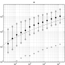
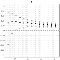
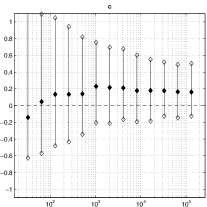
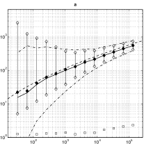
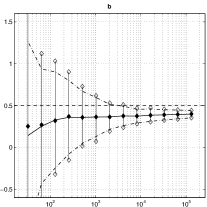
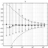
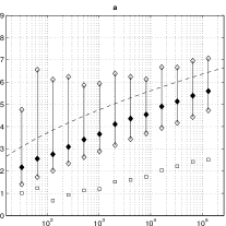
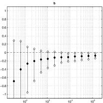
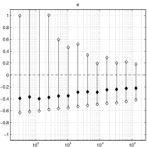
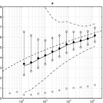
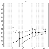
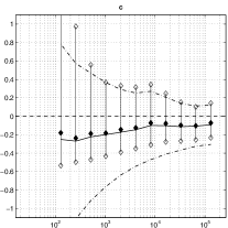
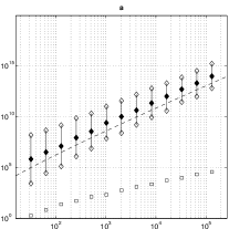
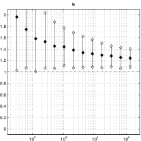
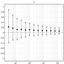
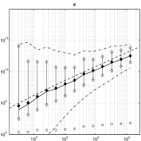
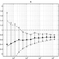
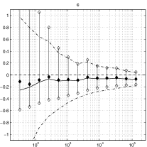
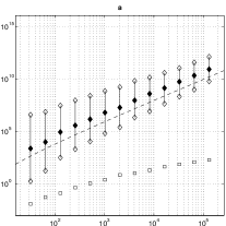
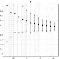
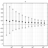
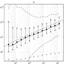
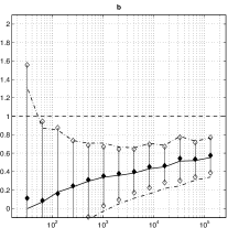
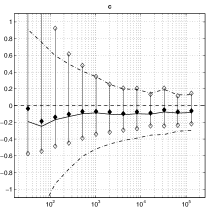
Figure 5.1 shows the results for the lognormal distribution with the GP-based estimator in the top row, and with the log-GW-based estimator in the bottom row. The leftmost column (a) shows the medians and the empirical 90%-intervals (between the 5% and 95% percentiles) of the quantile estimates; the width of an empirical 90%-interval will be referred to as “spread”. The quantiles $U(n^{2})$ to be estimated are indicated by a dashed curve. Approximate thresholds $U(n/k(n))$ and $U(n/k_{0}(n))$ are indicated by open squares. The middle column (b) shows the parameter estimates $\hat{\gamma}_{n}^{m}$ (top) and $\hat{\theta}_{n}$ (bottom), with the dashed lines indicating the tail indices $\gamma$ and $\theta$ for the distribution function considered. The rightmost column (c) displays the probability-based errors $\hat{\nu}_{n}^{m}$ (top) and $\hat{\nu}_{n}$ (bottom). For the log-GW-based estimator, also deterministic approximations $\tilde{q}_{y_{n}}(2\log n)$ with with $\tilde{\theta}=a_{\iota}$ and $\tilde{g}=g_{\iota}$ in (3.1) and asymptotic 90% intervals based on (4.18)-(4.20) are displayed. The latter are not confidence intervals, but are shown for comparison against the empirical 5% and 95% percentiles and medians of the (biased) estimates in order to verify how good the approximations provided by (4.18)-(4.20) are.

The top row of Figure 5.1 shows the GP-based estimates of $\log U(n^{2})$ apparently settling at a fixed distance upward from the exact values, and no convergence of $\hat{\nu}_{n}^{m}$. The parameter estimates $\hat{\gamma}_{n}^{m}$ appear to converge slowly. In the bottom row, the log-GW-based estimator is seen to perform well, with bias rapidly vanishing. Also, the spreads in $\hat{q}_{n}$ and $\hat{\nu}_{n}$ drop much more rapidly with increasing $n$ than for $\hat{q}_{n}^{m}$ and $\hat{\nu}_{n}^{m}$.

Figure 5.2 for the normal distribution displays a similar pattern as Figure 5.1, but with some differences. The GP-based estimator now underestimates the very high quantiles, even though the parameter estimator $\hat{\gamma}_{n}^{m}$ converges rapidly. This is the only case in which the sample maximum as lower bound to the quantile estimate became effective. The log-GW-based quantile estimator is performing much better in this case, although convergence is not as rapid as with lognormal data. Based on these results alone, it is not clear whether the bias in $\hat{\nu}_{n}$ converges to zero; deterministic computations (not shown) for $n$ up to ${\scriptstyle 2^{60}}$ with prescribed $k_{2}(n)={\scriptstyle\left\lfloor n^{1/4}\right\rfloor}$ show that it vanishes slowly. For $\hat{q}_{n}(2\log n)-q(2\log n)$, a small nonzero bias eventually remains, but the error relative to $q(2\log n)$ vanishes, and therefore also the error relative to $q(2\log n)-q(y_{n})$.

Since the favourable results of the log-GW-based estimator on lognormal data would translate directly to equivalent results with an analogous GW-based estimator on normal data, the latter would do better on the normal data than the log-GW-based quantile estimator in Figure 5.2. This indicates that in some cases, the speed of convergence may be increased by replacing the latter by a GW-based estimator.

The next two examples concern heavy-tailed distribution functions with classical Pareto tail limits $U\in ERV_{(0,\infty)}$. By Proposition 1(a), $\log q\in ERV_{\{1\}}$. Figure 5.3 shows results obtained for the distribution function satisfying $U(t)=t(1+2(\log t){}^{2})-1$. Concerning bias, both estimators perform rather well as expected. For small $n$, the log-GP-based estimator has a much smaller spread than the log-GW estimator; for large $n$, the spreads are similar. Given that the log-GW based estimator is based on only three order statistics, a large small-sample spread is not surprising. Indeed, replacing the moment estimator by Pickands’ estimator for $\gamma$ (Pickands, (1975)) based on three order statistics, the spread becomes larger than for the log-GW estimator (result not shown).

Finally, Figure 5.4 shows results for the Burr(1,$\frac{1}{4}$,4) distribution with $U(t)={\scriptstyle(t^{1/4}-1)^{4}}$, which also satisfies $U\in ERV_{\{1\}}$. Unlike the previous examples, $U$ has a negative second-order index (see de Haan & Ferreira, (2006)) in this case, so eventually, convergence toward the GP limit should be rapid. As in the previous example, the GP-based estimator performs rather well; the log-GW-based estimator performs similarly but with somewhat larger spread (which is again smaller than obtained when using Pickands’ estimator for the GP-based estimation).

In all figures, the threshold values $U(n/k_{0}(n))$ and $U(n/k(n))$ corresponding to the numbers $k_{0}(n)$ and $k(n)$ of upper order statistics used by the estimators are rather different for the two estimators. For the log-GW estimator with $\iota=2$, $k_{0}(n)$ must be at least $n^{3/4}$ irrespective of $k_{2}(n)$ (see (4.1)), so there is little room for adjustment in order to optimise performance. However, with the GP estimator, $k(n)$ can be reduced considerably to reduce bias if needed. For the lognormal and normal distributions in Figures 5.1 and 5.2, this is seen to lead to a large spread.

The results tentatively confirm the expectations. For distribution functions in the classical Pareto ($\gamma>0$) domain of attraction (satisfying $\log q\in ERV_{\{1\}}$), log-GW en GP-based estimators seem to perform similarly. However, in the classical domain of attraction of the exponential ($\gamma=0$), log-GW may offer advantages.

For the log-GW-based estimator, the asymptotic 90%-intervals for for $\hat{\theta}_{n}$ and $\hat{\nu}_{n}$ based on (4.18) and (4.19) provide good approximations to the empirical 90%-intervals. For $\hat{q}_{n}$, the asymptotic 90% intervals based on (4.20) are in some cases much too wide.

6 Discussion

The log-GW tail limit $\log q\in ERV$ is a weak assumption of the same nature as the classical regularity assumption $U\in ERV$ corresponding to the GP tail limit, but specifically aimed toward approximation and estimation of very high quantiles for probabilities in the range (1.5). Proposition 1 indicates that if a GP tail limit applies, then log-GW-based approximation may provide benefits if $\gamma=0$. If $\gamma>0$, then approximation using the GP tail should already be adequate.

Further analysis confirms this: if $U\in ERV_{\{0\}}$ and $\log q\in ERV$, then $\log q\in ERV_{(-\infty,1]}$ (see Theorem 2.2(b)), offering a continuum of tail shapes for approximation of quantiles where the GP limit with $\gamma=0$ offers only one, the exponential tail.

Suppose that $U\in ERV_{\{0\}}$. Then any assumption ensuring convergence of GP-based quantile approximations with $\gamma=0$ as in (2.8) implies $q\in RV_{\{1\}}$, so $\log q\in ERV_{\{0\}}(1)$ (see Proposition 1(b)); therefore, it excludes all other distribution functions satisfying a log-GW tail limit and a GP tail limit with $\gamma=0$, such as Weibull-like distributions (e.g. the normal distribution), distribution functions of exponents of Weibull-like distributed random variables (e.g. the lognormal distribution), light tails with $q(\infty)$ still infinite such as $F=1-\exp(-\exp\textrm{I{d}})$, distribution functions with finite $q(\infty)$ such as $F=1-\exp((q(\infty)-\textrm{Id})^{1/\theta}$) with $\theta<0$, just to mention a few which correspond to log-GW or GW limits or are close to such limits.

As an example, consider the following seemingly innocent rate assumption for (1.2):

$$\lim_{t\rightarrow\infty}\biggl{(}\frac{U(t\lambda)-U(t)}{w(t)}-h_{\gamma}(\lambda)\biggr{)}\log t=0\quad\forall\lambda\geq 1$$ (6.1)

with $\gamma=0$. It implies $q\in ERV_{\{1\}}$ (see Subsection 7.8), and thus by Lemma 1(a) in Subsection 7.9, $\log q\in ERV_{\{0\}}(1)$. Therefore, in the present context, (6.1) is actually quite restrictive.

The Pareto domain of attraction with $\gamma>0$ is in the domain of attraction of the log-GW tail limit $\log q\in ERV_{\{1\}}$ (Proposition 1(a)), so all results obtained for the latter also apply to the former. Therefore, one might expect that if log-GW based quantile approximation and estimation can not offer improvement if $\gamma>0$, it may not do much harm either.

This is tentatively confirmed by the results of the simulations in Section 5, which indicate that log-GW-based quantile estimation may have merits within the $\gamma=0$ subdomain of attraction of the GP limit and performs similarly to GP-based quantile estimation in the $\gamma>0$ subdomain. However, it would be premature to draw conclusions from only these few examples.

For the log-GW based estimator $\hat{q}_{n}$, the log-GW limit is sufficient for consistency. To establish asymptotic normality, a relatively high rate of convergence (4.21) to the log-GW limit needed to be assumed. As shown in Section 4, this is a consequence of the particular formulation of this estimator. Therefore, there is a need for alternative estimators which allow the rate condition (4.21) to be relaxed. Based on the simulation results, there appears to be a need for improved accuracy with small sample sizes as well. It is suggested in Section 4 that bias correction based on estimation of a higher-order ERV model could be useful in log-GW-based estimators in order to obtain asymptotic normality while avoiding slow decay of variability with increasing $n$.

A limitation of log-GW approximation and estimation is that the notions of convergence in (3.4) and (4.13) may be weak and cannot be replaced by (3.6) and (4.14) for tails heavier than a typical Weibull tail unless additional assumptions apply. The probability-based errors (3.9) and (4.12) are based on log-ratios of survival functions of a quantile and its approximation or estimator. Although natural in view of the probability range considered, a stronger notion of convergence, e.g. of a ratio of survival functions, would be desirable for applications. Stronger notions of convergence apply under the additional assumptions for establishing asymptotic normality for the quantile estimator $\hat{q}_{n}$ in Corollary 1, notably the rate assumption (4.21); see Remark 5.

As a final remark, log-GW-based quantile approximation and estimation for light tails with finite endpoints has only been marginally covered here, so this case remains to be examined in more detail.

7 Proofs and lemmas

7.1 Proof of Proposition 1

If $U\in ERV_{\{\gamma\}}$ for $\gamma>0$, then $U\in RV_{\{\gamma\}}$ so by the Potter bounds (e.g. Bingham et al, (1987), Theorem 1.5.6), there is for every $\varepsilon\in(0,\gamma\wedge 1)$ a $y_{\varepsilon}>0$ such that $y(\lambda-1)(\gamma-\varepsilon)-\varepsilon\leq\log q(y\lambda)-\log q(y)\leq y(\lambda-1)(\gamma+\varepsilon)+\varepsilon$ for all $y\geq y_{\varepsilon}$ and all $\lambda\geq 1$. Therefore, $\log q\in ERV_{\{1\}}(\textrm{Id}\cdot\gamma)$, so $\log q\in RV_{\{1\}}$. Noting that $\gamma y\sim\log q(y)$ as $y\rightarrow\infty$ and $\gamma U(t)/w(t)\rightarrow 1$ as $t\rightarrow\infty$ (both due to de Haan & Ferreira, (2006), Theorem B.2.2(1)), we obtain $\log\tilde{U}_{t}(t^{\lambda})=\log U(t)+\log(1+\frac{w(t)}{\gamma U(t)}(t^{(\lambda-1)\gamma}-1)))$ $=\log U(t)+(\lambda-1)\gamma\log t+o(1)\sim\lambda\log U(t)$ for every $\lambda\geq 1$, and since $\log q\in RV_{\{1\}}$, (2.7) follows, so (a) is proven.

If $\gamma=0$, (2.8) implies $\lim_{y\rightarrow\infty}(q(y\lambda)-q(y))/(w(\textrm{e}^{y})y)=\lambda-1\quad\forall\lambda>1$. Therefore, $q\in ERV_{\{1\}}$ and by Lemma 1(a) in Subsection 7.9, $\log q\in ERV_{\{0\}}(1)$, proving (b).

7.2 Proof of Theorem 2.2

Suppose that $U\in ERV_{\{\gamma\}}$ with $\gamma>0$, then as in Subsection 7.1, there is for every $\varepsilon\in(0,\gamma\wedge 1)$ a $y_{\varepsilon}>0$ such that $y(\lambda-1)(\gamma-\varepsilon)-\varepsilon\leq\log(q(y\lambda)/q(y))\leq y(\lambda-1)(\gamma+\varepsilon)+\varepsilon$ for all $y\geq y_{\varepsilon}$ and all $\lambda\geq 1$, and therefore, fixing $\iota>1$ and $\xi>\iota$, there is some $\varepsilon\in(0,\gamma(\xi-\iota)/(\xi+\iota-2)\wedge 1)$, $\delta>0$ and $z_{\varepsilon}\geq y_{\varepsilon}$ such that

$$\frac{q(y\xi)-q(y)}{q(y\iota)-q(y)}\geq\frac{e^{y(\xi-1)(\gamma-\varepsilon)}(1-\varepsilon)-1}{e^{y(\iota-1)(\gamma+\varepsilon)}(1+\varepsilon)-1}\geq\exp(\delta y)\quad\forall y\geq z_{\varepsilon}.$$ (7.1)

However, since $q\in ERV$, the left-hand side of (7.1) must tend to $h_{\theta}(\xi)/h_{\theta}(\iota)<\infty$ for some real $\theta$ as $y\rightarrow\infty$, so $\gamma$ cannot exceed $0$. Assuming that $\gamma<0$, a similar argument leads to a similar contradiction, completing the proof of (a).

For (b), if $U\in ERV$ then by Lemma 1(a) in Subsection 7.9, $\log U\in ERV$ so since $\log q\in ERV$, (a) implies that $\log U\in ERV_{\{0\}}$. Since $U\in ERV$ and $\log q\in ERV$, Proposition 1(a) implies that either $U\in ERV_{(0,\infty)}$ and $\log q\in ERV_{\{1\}}$, or $U\in ERV_{(-\infty,0]}$. In the latter case, since $\log U\in ERV_{\{0\}}$, Lemma 1(c) implies that $U\in ERV_{\{0\}}\subset RV_{\{0\}}$. Therefore, by the Potter bounds, $\log q(y)=o(y)$ as $y\rightarrow\infty$, so again by the Potter bounds, $\log q$ cannot be in $RV_{(1,\infty)}=ERV_{(1,\infty)}$.

7.3 Proof of Proposition 2

Because $\tilde{\theta}(y)\rightarrow\theta$ and $\tilde{g}(y)\sim g(y)$ as $y\rightarrow\infty$, noting that by (1.4), $h_{\theta+o(1)}(\lambda)=\lambda^{o(1)}h_{\theta}(\lambda)$, we obtain using the mean value theorem,

$$\log\tilde{q}_{y}(y\lambda)=\log q(y)+g(y)h_{\theta}(\lambda)(1+o(1))$$ (7.2)

locally uniformly in $\lambda>0$. Since (2.9) also holds locally uniformly in $\lambda>0$ (see Bingham et al, (1987), Theorem 3.1.16), (3.4) follows from (7.2). If in addition, (3.5) holds, then by (3.4), $\log\tilde{q}_{y}(y\lambda)-\log q(y\lambda)=(\tilde{q}_{y}(y\lambda)/q(y\lambda)-1)(1+o(1))$ as $y\rightarrow\infty$ locally uniformly in $\lambda>0$, and (3.6) follows. If $q\in ERV$, then (3.5) follows from Lemma 1(b) in Subsection 7.9.

7.4 Clarification of Remark 1

Under condition (3.5), $q(y)g(y)$ in (3.6) can be replaced by $q(y\xi)-q(y)$ for any $\xi\in(0,\infty)\setminus\{1\}$: for $\xi>1$, this follows from (3.7), as $q(y\xi)/q(y)-1>\log q(y\xi)-\log q(y)$; for $\xi\in(0,1)$, we find $\bigl{|}\frac{g(y)q(y)}{q(y\xi)-q(y)}\bigr{|}=\frac{g(y\xi)}{q(y)/q(y\xi)-1}O(1)=\frac{g(y\xi)}{\log q(y)-\log q(y\xi)}O(1)=O(1)$ as $y\rightarrow\infty$ by regular variation of $g$ and (3.7).

If $q(\infty)<\infty$, then $q(y)g(y)$ in (3.6) may be replaced by $q(\infty)-q(y\eta)$ for any $\eta>0$: taking $\xi>1$, $\frac{q(y)g(y)}{q(\infty)-q(y\eta)}\leq\frac{q(\infty)g(y)}{q(y\eta\xi)-q(y\eta)}\sim\frac{g(y\eta)}{\log q(y\eta\xi)-\log q(y\eta)}\frac{g(y)}{g(y\eta)}=O(1)$ as $y\rightarrow\infty$ by (3.7) and regular variation of $g$.

7.5 Proof of Theorem 3.1

From Proposition 2 and (2.3), as $y\rightarrow\infty$,

$$\log\tilde{q}_{y}(y\lambda)=\log q(y)+g(y)(h_{\theta}(\lambda)+o(1))$$ (7.3)

locally uniformly in $\lambda>0$. Let $\varLambda>1$ and $b\in(0,\varLambda^{-\bigl{|}\theta\bigr{|}}/\bigl{|}\theta\bigr{|})$. Applying the mean value theorem to $x\mapsto h_{\theta}^{-1}(h_{\theta}(\lambda)+x)=(\lambda^{\theta}+x\theta)^{1/\theta}$, we find that for some $M>0$,

$$\bigl{|}h_{\theta}^{-1}(h_{\theta}(\lambda)+x)-\lambda\bigr{|}\leq M\bigl{|}x\bigr{|}\qquad\forall\lambda\in[\varLambda^{-1},\varLambda],\>x\in[-b,b].$$

Therefore, by (7.3), $\log\tilde{q}_{y}(y\lambda)=\log q(y)+g(y)h_{\theta}(\lambda+o(1))$ uniformly in $\lambda\in[\varLambda^{-1},\varLambda]$, so using (2.4),

$$q^{-1}(\tilde{q}_{y}(y\lambda))=-\log\bigl{(}1-F\bigl{(}q(y)e^{g(y)h_{\theta}(\lambda+o(1))}\bigr{)}\bigr{)}=y(\lambda+o(1))$$

uniformly in $\lambda\in[\varLambda^{-1},\varLambda]$. As $\lim_{z\rightarrow\infty}z^{-1}q^{-1}(q(z))=1$ by (2.4), we obtain (3.9).

7.6 Proof of Theorem 4.1

Define $\hat{\iota}_{m}(n)$ for all $n\geq 1$ and $m\in\{0,1,2\}$ by

$$\hat{\iota}_{m}(n):=y_{n}^{-1}q^{-1}(X_{n-k_{m}(n)+1,n})=-y_{n}^{-1}\log(1-F(X_{n-k_{m}(n)+1,n})).$$ (7.4)

To simplify notation, we will use

$$s:=\log q,\quad\hat{s}_{n}:=\log\hat{q}_{n},\quad\tilde{s}_{y}:=\log\tilde{q}_{y}.$$ (7.5)

Since $q(\infty)>1$, almost surely some $n_{0}\in\mathbb{N}$ exists such that for all $n\geq n_{0}$, $X_{n-k_{0}(n)+1,n}>0$ and $\hat{q}_{n}(z)$ is defined. By Lemma 2 in Subsection 7.9, (7.25) and (7.26) hold for $\hat{\iota}_{0}(n)$, $\hat{\iota}_{1}(n)$ and $\hat{\iota}_{2}(n)$ defined by (7.4). Therefore, by (4.3) and (7.25), using (7.5),

$$\hat{\theta}_{n}=\frac{1}{\log\iota}\log\frac{s(y_{n}\hat{\iota}_{2}(n))-s(y_{n}\hat{\iota}_{1}(n))}{s(y_{n}\hat{\iota}_{1}(n))-s(y_{n}\hat{\iota}_{0}(n))}\quad\forall n\geq n_{0}\quad\textrm{a.s}.$$

and as $s\in ERV_{\{\theta\}}(g)$ and therefore $g\in RV_{\{\theta\}}$, by locally uniform convergence (see Bingham et al, (1987), Theorems 3.1.16 and 1.5.2), and (7.26), almost surely

$$\hat{\theta}_{n}=\frac{1}{\log\iota}\left(\log\frac{h_{\theta}(\hat{\iota}_{2}(n)/\hat{\iota}_{1}(n))+o(1)}{h_{\theta}(\hat{\iota}_{1}(n)/\hat{\iota}_{0}(n))+o(1)}+\log\frac{g(y_{n}\hat{\iota}_{1}(n))}{g(y_{n}\hat{\iota}_{0}(n))}\right)\rightarrow\theta.$$ (7.6)

Similarly, using (7.6), almost surely

$$\frac{\hat{g}_{n}}{g(y_{n})}=\frac{s(y_{n}\hat{\iota}_{1}(n))-s(y_{n}\hat{\iota}_{0}(n)\eta)}{g(y_{n})h_{\hat{\theta}_{n}}(\iota)}=\frac{h_{\theta}(\hat{\iota}_{1}(n)/\hat{\iota}_{0}(n))+o(1)}{h_{\hat{\theta}_{n}}(\iota)}\left(\frac{g(y_{n}\hat{\iota}_{0}(n))}{g(y_{n})}\right)\rightarrow 1,$$

so (4.11) is proven. Furthermore, in a similar manner, almost surely

$$\frac{s(y_{n})-\log X_{n-k_{0}(n)+1,n}}{g(y_{n})}=\frac{s(y_{n})-s(y_{n}\hat{\iota}_{0}(n))}{g(y_{n})}=-h_{\theta}(\hat{\iota}_{0}(n))+o(1)\rightarrow 0.$$ (7.7)

By (4.11), almost surely $(\hat{g}_{n}/g(y_{n}))h_{\hat{\theta}_{n}}(\lambda)\rightarrow h_{\theta}(\lambda)$ locally uniformly in $\lambda>0$, so using (7.7), $\hat{s}_{n}$ defined by (7.5) and (4.2) satisfies

$$\sup_{\lambda\in[\Lambda^{-1},\Lambda]}\bigl{|}\hat{s}_{n}(y_{n}\lambda)-s(y_{n}\lambda)\bigr{|}/g(y_{n})\rightarrow 0\qquad a.s.\qquad\forall\varLambda>1.$$ (7.8)

Using (4.9), we subsequently obtain (4.13), and (4.14) follows readily as in the proof of Proposition 2. From (7.8) and (2.3), almost surely

$$\hat{s}_{n}(y_{n}\lambda)=s(y_{n}\lambda)+o(g(y_{n}))=s(y_{n})+g(y_{n})(h_{\theta}(\lambda)+o(1))$$ (7.9)

locally uniformly in $\lambda>0$. By mimicking the proof of Theorem 3.1 in Subsection 7.5 with $y_{n}$ replacing $y$ and $\hat{s}_{n}(y_{n}\lambda)$ replacing $\tilde{s}_{y}(y\lambda)$, we obtain that for every $\varLambda>1$ almost surely, $\sup_{\lambda\in[\Lambda^{-1},\Lambda]}\bigl{|}\hat{\nu}_{n}(y_{n}\lambda)\bigr{|}\rightarrow 0$; using (4.9), (4.12) follows.

7.7 Proofs of Theorem 4.2 and Corollary 1

Using the definitions (7.5), by (4.15), $s^{\prime}\in RV_{\{\theta-1\}}$, so $s$ is a homeomorphism on some neighbourhood of $\infty$. Therefore, without loss of generality, we can take $s$ increasing and continuous, so $\log X_{n-k_{m}(n)+1,n}=s(y_{n}\hat{\iota}_{m}(n))$ for all $n$ and $m\in\{0,1,2\}$. Furthermore, by integration, $s^{\prime}\in RV_{\{\theta-1\}}$ implies

$$s(y\lambda)-s(y)=s^{\prime}(y)yh_{\theta}(\lambda)(1+o(1))$$ (7.10)

with $o(1)$ vanishing locally uniformly for $\lambda>0$ as $y\rightarrow\infty$. Therefore, with $\hat{\iota}$ as in (7.4) and

$$\mathcal{R}_{n}^{m}:=\frac{\log X_{n-k_{m}(n)+1,n}-s(y_{n}\iota^{m})}{s^{\prime}(y_{n}\iota^{m})y_{n}\iota^{m}},$$

using (7.26) from Lemma 2 in Subsection 7.9, almost surely

$$\mathcal{R}_{n}^{m}=\frac{s(y_{n}\hat{\iota}_{m}(n))-s(y_{n}\iota^{m})}{s^{\prime}(y_{n}\iota^{m})y_{n}\iota^{m}}\sim h_{\theta}(\iota^{-m}\hat{\iota}_{m}(n))\sim\iota^{-m}\hat{\iota}_{m}(n)-1$$ (7.11)

for $m\in\{0,1,2\}$. Similarly, for $\tilde{\nu}$ defined by (3.8) with $\tilde{\theta}=a_{\iota}$ and $\tilde{g}=g_{\iota}$ in (3.1), substituting $y_{n}\lambda(1+\tilde{\nu}_{y_{n}}(y_{n}\lambda))$ for $y$ in (7.10) and using $s^{\prime}\in RV_{\{\theta-1\}}$ and Theorems 3.1 and 4.1, almost surely,

$$\frac{s(y_{n}\lambda(1+\hat{\nu}_{n}(y_{n}\lambda)))-s(y_{n}\lambda(1+\tilde{\nu}_{y_{n}}(y_{n}\lambda)))}{s^{\prime}(y_{n})y_{n}}\sim\lambda{}^{\theta}h_{\theta}\left(\frac{1+\hat{\nu}_{n}(y_{n}\lambda)}{1+\tilde{\nu}_{y_{n}}(y_{n}\lambda)}\right)$$

$$\sim\lambda^{\theta}(\hat{\nu}_{n}(y_{n}\lambda)-\tilde{\nu}_{y_{n}}(y_{n}\lambda))$$ (7.12)

locally uniformly for $\lambda>0$. From (3.3) and (4.3), using (7.11), (7.10), $s^{\prime}\in RV_{\{\theta-1\}}$ and (7.26),

$$(\hat{\theta}_{n}-a_{\iota}(y_{n}))\log\iota=\log\left(1+\frac{\mathcal{R}_{n}^{2}\frac{s^{\prime}(y_{n}\iota^{2})\iota}{s^{\prime}(y_{n}\iota)}-\mathcal{R}_{n}^{1}}{\frac{s(y_{n}\iota^{2})-s(y_{n}\iota)}{y_{n}\iota s^{\prime}(y_{n}\iota)}}\right)-\log\left(1+\frac{\mathcal{R}_{n}^{1}\frac{s^{\prime}(y_{n}\iota)\iota}{s^{\prime}(y_{n})}-\mathcal{R}_{n}^{0}}{\frac{s(y_{n}\iota)-s(y_{n})}{y_{n}s^{\prime}(y_{n})}}\right)$$

$$=\left(h_{\theta}(\iota)\right)^{-1}\left(\iota^{\theta}(\iota^{-2}\hat{\iota}_{2}(n)-1)(1+o(1))-(\iota^{-1}\hat{\iota}_{1}(n)-1)(1+o(1))\right.$$

$$\left.-\iota^{\theta}(\iota^{-1}\hat{\iota}_{1}(n)-1)(1+o(1))+(\hat{\iota}_{0}(n)-1)(1+o(1))\right)\quad\textrm{a.s.}$$ (7.13)

Because $1-F(X)$ has the uniform distribution on $(0,1)$, by Smirnov, (1952),

$$y_{n}(\hat{\iota}_{m}(n)-\iota^{m})\sqrt{k_{m}(n)}\overset{d}{\rightarrow}N(0,1)\quad\forall m\in\{0,1,2\}$$ (7.14)

as $n\rightarrow\infty$. Therefore, as $k_{2}(n)=o(k_{1}(n))$ and $k_{1}(n)=o(k_{0}(n))$, (7.13) implies (4.18). From (4.2) and (3.1),

$$\frac{\hat{s}_{n}(y_{n}\lambda)-\tilde{s}_{y_{n}}(y_{n}\lambda)}{y_{n}s^{\prime}(y_{n})}=\mathcal{R}_{n}^{0}+\frac{h_{a_{\iota}(y_{n})}(\lambda)}{h_{a_{\iota}(y_{n})}(\iota)}\left(\mathcal{R}_{n}^{1}\frac{s^{\prime}(y_{n}\iota)\iota}{s^{\prime}(y_{n})}-\mathcal{R}_{n}^{0}\right)$$ (7.15)

$$+\left(\frac{h_{\hat{\theta}_{n}}(\lambda)}{h_{\hat{\theta}_{n}}(\iota)}-\frac{h_{a_{\iota}(y_{n})}(\lambda)}{h_{a_{\iota}(y_{n})}(\iota)}\right)\left(\frac{s(y_{n}\iota)-s(y_{n})}{y_{n}s^{\prime}(y_{n})}+\mathcal{R}_{n}^{1}\frac{s^{\prime}(y_{n}\iota)\iota}{s^{\prime}(y_{n})}-\mathcal{R}_{n}^{0}\right).$$

As $s$ is increasing and $\sqrt{k_{2}(n)/k_{m}(n)}\log\log n\rightarrow 0$ for $m\in\{0,1\}$, Lemma 2(b) in Subsection 7.9 implies that

$$(\hat{\iota}_{m}(n)-\iota^{m})y_{n}\sqrt{k_{2}(n)}\rightarrow 0\quad m\in\{0,1\}\quad a.s.$$ (7.16)

and $(\hat{\iota}_{2}(n)-\iota^{2})y_{n}\sqrt{k_{2}(n)}=o(\log\log n)$ a.s., so by (7.13), $(\hat{\theta}_{n}-a_{\iota}(y_{n}))y_{n}\sqrt{k_{2}(n)}=o(\log\log n)$ a.s. Therefore, by Taylor’s theorem (see (4.17)),

$$\left|\frac{h_{\hat{\theta}_{n}}(\lambda)}{h_{\hat{\theta}_{n}}(\iota)}-\frac{h_{a_{\iota}(y_{n})}(\lambda)}{h_{a_{\iota}(y_{n})}(\iota)}-\kappa_{\theta}(\lambda,\iota)(\hat{\theta}_{n}-a_{\iota}(y_{n}))\right|=O(1)(\hat{\theta}_{n}-a_{\iota}(y_{n}))^{2}\quad a.s.$$ (7.17)

locally uniformly in $\lambda>0$, with on the right-hand side (using (4.8)):

$$(\hat{\theta}_{n}-a_{\iota}(y_{n}))^{2}=o(1)(\log\log n)^{2}/(y_{n}^{2}k_{2}(n))=o(1)/(y_{n}k_{2}(n))\quad a.s.$$ (7.18)

By (7.11) and (7.16), $\mathcal{R}_{n}^{m}y_{n}\sqrt{k_{2}(n)}\rightarrow 0$ a.s. for $m\in\{0,1\}$. Therefore, from (7.15), using (7.17), (7.18), (7.10) and $s^{\prime}\in RV_{\{\theta-1\}}$, for all $\Lambda>1$,

$$\sup_{\lambda\in[\Lambda^{-1},\Lambda]}\left|\frac{\hat{s}_{n}(y_{n}\lambda)-\tilde{s}_{y_{n}}(y_{n}\lambda)}{y_{n}s^{\prime}(y_{n})}-\kappa_{\theta}(\lambda,\iota)(\hat{\theta}_{n}-a_{\iota}(y_{n}))h_{\theta}(\iota)\right|y_{n}\sqrt{k_{2}(n)}\rightarrow 0\quad a.s.$$ (7.19)

Therefore, by (4.18) and (4.9), (4.20) is obtained. Because $s$ is continuously increasing, $s(y_{n}\lambda(1+\tilde{\nu}_{y_{n}}(y_{n}\lambda)))=\tilde{s}_{y_{n}}(y_{n}\lambda)$ and $s(y_{n}\lambda(1+\hat{\nu}_{n}(y_{n}\lambda)))=\hat{s}_{n}(y_{n}\lambda)$ in (7.12) so almost surely,

$$\hat{\nu}_{n}(y_{n}\lambda)-\tilde{\nu}_{y_{n}}(y_{n}\lambda)=(1+o(1))\lambda^{-\theta}\frac{\hat{s}_{n}(y_{n}\lambda)-\tilde{s}_{y_{n}}(y_{n}\lambda)}{y_{n}s^{\prime}(y_{n})}$$

locally uniformly in $\lambda>0$. Therefore, using (4.9) and (4.20), we obtain (4.19). This proves Theorem 4.2.

To prove Corollary 1, note that (4.21) must hold locally uniformly in $\lambda\geq 1$: with $r$ defined by $r(y):=\log s^{\prime}(y)-(\theta-1)\log y$, (4.21) is equivalent to $\lim_{y\rightarrow\infty}(r(y\lambda)-r(y))\phi(y)=0$ for all $\lambda\geq 1$, which holds locally uniformly in $\lambda\geq 1$ by Theorem 3.1.7c of Bingham et al, (1987). By integration,

$$s(y\lambda)-s(y)=ys^{\prime}(y)h_{\theta}(\lambda)(1+o(1)/\phi(y))$$ (7.20)

locally uniformly in $\lambda\geq 1$. Therefore,

$$a_{\iota}(y)=\theta+o(1)/\phi(y),$$ (7.21)

so by the mean value theorem, $\frac{h_{a_{\iota}(y)}(\lambda)}{h_{a_{\iota}(y)}(\iota)}-\frac{h_{\theta}(\lambda)}{h_{\theta}(\iota)}=O(a_{\iota}(y)-\theta)=o(1)/\phi(y)$ locally uniformly in $\lambda\geq 1$. Using (7.20), therefore,

$$\frac{\tilde{s}_{y}(y\lambda)-s(y\lambda)}{ys^{\prime}(y)}=\frac{s(y\iota)-s(y)}{ys^{\prime}(y)}\Bigl{(}\frac{h_{\theta}(\lambda)}{h_{\theta}(\iota)}+o(1)/\phi(y)\Bigr{)}+\frac{s(y)-s(y\lambda)}{ys^{\prime}(y)}=o(1)/\phi(y)$$ (7.22)

locally uniformly in $\lambda\geq 1$. Finally, by (7.10) and Theorem 3.1, as $s^{\prime}\in RV_{\{\theta-1\}}$,

$$s(y\lambda(1+\tilde{\nu}_{y}(y\lambda)))-s(y\lambda)\sim\lambda^{\theta}h_{\theta}\left(1+\tilde{\nu}_{y}(y\lambda)\right)ys^{\prime}(y)\sim\lambda^{\theta}\tilde{\nu}_{y}(y\lambda)ys^{\prime}(y)$$ (7.23)

locally uniformly in $\lambda\geq 1$. Since $s$ is continuously increasing, $s(z(1+\tilde{\nu}_{y}(z)))=\tilde{s}_{y}(z)$ for all $z>0$, so combining (7.23) and (7.22), it follows that

$$\tilde{\nu}_{y}(y\lambda)=o(1)/\phi(y)$$ (7.24)

locally uniformly in $\lambda\geq 1$. Using $k_{2}(n)=O(\phi^{2}(y_{n})y_{n}^{-2})$, (4.22) follows from (4.18) and (7.21); using (4.9) as well, (4.24) follows from (4.20) and (7.22), and (4.23) follows from (4.19) and (7.24).

7.8 Proof that (6.1) implies $q\in ERV_{\{1\}}$

Take $w\in RV_{\{0\}}$. With $R_{\lambda}(t):=(U(t\lambda)-U(t))/w(t)$, (6.1) implies $w(t\lambda)/w(t)=(R_{\lambda\xi}(t)-R_{\lambda}(t))/R_{\xi}(t\lambda)=1+o(1/\log t)$ for all $\lambda\geq 1$ and $\xi>1$, so by Bojanic & Seneta, (1971) (see Bingham et al, (1987), Theorem 2.3.1), $w(t^{\lambda})/w(t)\rightarrow 1$ locally uniformly in $\lambda\geq 1$ as $t\rightarrow\infty$; applying Theorem 3.6.6 in Bingham et al, (1987) gives $U(t^{\lambda})-U(t)\sim(\lambda-1)w(t)\log t$ for all $\lambda\geq 1$, so $q\in ERV_{\{1\}}$.

7.9 Lemmas

Lemma 1

Let $f$ be a nondecreasing function satisfying $f(\infty)>0$.

(a) If $f\in ERV_{\{\theta\}}$, then $\log f\in ERV_{\{\min(\theta,0)\}}(g)$ with the positive function $g$ converging to $\max(\theta,0)$.

(b) If $\log f\in ERV_{\{\theta\}}(g)$, then $f\in ERV$ if and only if $g$ converges to some $g_{\infty}\in[0,\infty)$. If so, then $f\in ERV_{\{\min(\theta,0)+\max(0,g_{\infty})\}}(fg)$.

(c) For $\theta<0$, $\log f\in ERV_{\{\theta\}}$ if and only if $f\in ERV_{\{\theta\}}$.

Proof

If $f\in ERV_{\{\theta\}}$ with $\theta>0$, then $f\in RV_{\{\theta\}}$ so $\log q\in ERV_{\{0\}}(\theta)$. If $f\in ERV_{\{\theta\}}(\bar{g})$ with $\theta\leq 0$, then as $y\rightarrow\infty$, $\bar{g}(y)/f(y)\rightarrow 0$ (see de Haan & Ferreira, (2006), Lemma 1.2.9). Therefore, for every $\lambda\in(0,1)\cup(1,\infty)$, also $f(y\lambda)/f(y)-1\rightarrow 0$, so $\log f(y\lambda)-\log f(y)\sim f(y\lambda)/f(y)-1$ and as $\bar{g}(y)/f(y)\rightarrow 0$, we obtain $\log f\in ERV_{\{\theta\}}(\bar{g}/f)$, proving (a).

If $g$ converges to $g_{\infty}>0$, then $f\in RV_{\{g_{\infty}\}}$, so $f\in ERV_{\{g_{\infty}\}}(fg)$. If $g$ converges to $0$, then for every $\lambda\in(0,1)\cup(1,\infty)$, $f(y\lambda)/f(y)-1\rightarrow 0$, so $f(y\lambda)/f(y)-1\sim\log f(y\lambda)-\log f(y)$ as $y\rightarrow\infty$. Therefore, $f\in ERV_{\{\theta\}}(fg)$ and necessarily, $\theta\leq 0$. This proves the “if” part of (b); the “only if” part follows from (a), and (c) follows directly from (a) and (b). ∎

Lemma 2

(a) $\hat{\iota}$ defined by (7.4) with (4.1) satisfies

$$X_{n-k_{m}(n)+1,n}=q(y_{n}\hat{\iota}_{m}(n))\quad\forall m\in\{0,1,2\},\>n\in\mathbb{N}\quad\textrm{a.s.}$$ (7.25)

(b) Let $k_{2}:\mathbb{\mathbb{N}\rightarrow N}$ satisfy (4.7) and $k_{2}(n)/\log\log n\rightarrow\infty$. If $q\in ERV$, then

$$\hat{\iota}_{m}(n)\rightarrow\iota^{m}\quad\forall m\in\{0,1,2\}\quad\textrm{a.s.}$$ (7.26)

If $F$ is continuous, then

$$(\hat{\iota}_{m}(n)-\iota^{m})y_{n}\sqrt{k_{m}}/\log\log n\rightarrow 0\quad\forall m\in\{0,1,2\}\quad\textrm{a.s.}$$ (7.27)

Proof

Almost surely, $X_{n-k+1,n}=q(-\log\mathcal{U}_{k,n})$ for all $n\in\mathbb{N}$ and $k\in\{1,...,n\}$, with $\mathcal{U}_{k,n}$ the $k^{th}$ order statistic of a sample of $n$ independent random variables uniformly distributed on $(0,1)$. Therefore, by (7.4),

$$\hat{\iota}_{m}(n)y_{n}=q^{-1}(q(-\log\mathcal{U}_{k_{m}(n),n}))\quad\forall m\in\{0,1,2\},\>n\in\mathbb{N}\quad a.s.$$ (7.28)

and (7.25) follows. For (b), note that $k_{m}(n)/n\rightarrow 0$ and $k_{m}(n)/\log\log n\rightarrow\infty$ for each $m\in\{0,1,2\}$, so by Einmahl & Mason, (1988) (Theorem 3(III) with $\nu=\frac{{\scriptstyle 1}}{2}$),

$$\left((n/k_{m}(n))\mathcal{U}_{k_{m}(n),n}-1\right)\sqrt{k_{m}}/\log\log n\rightarrow 0\quad\forall m\in\{0,1,2\}\quad\textrm{a.s.}$$

and as (4.7) implies that $(\log(n/k_{m}(n))-\iota^{m}y_{n})=O(1/k_{m}(n))$ for $m=0,1,2$,

$$(\log\mathcal{U}_{k_{m}(n),n}+\iota^{m}y_{n})\sqrt{k_{m}}/\log\log n\rightarrow 0\quad\forall m\in\{0,1,2\}\quad\textrm{a.s.}$$ (7.29)

If $F$ is continuous, then $q^{-1}\circ q=\textrm{Id}$, so (7.27) follows from (7.28) and (7.29). If not, then $\hat{\iota}_{m}(n)=y_{n}^{-1}q^{-1}(q(\iota^{m}y_{n}+o(1)))$ a.s. by (7.28) and (7.29), so if $q\in ERV$, then (7.26) follows from (2.10). ∎

Conflict of Interest The author declares that he has no conflict of interest.

References

- Adams & Atkinson, (2003) Adams, J. and G. Atkinson, “Development of seismic hazard maps for the proposed 2005 edition of the National Building Code of Canada”. Can. J. Civ. Eng. 30: 255–271, (2003)
- Bingham et al, (1987) Bingham. N.H., C.M. Goldie, J.L. Teugels, Regular variation. Cambridge Univ. Press, (1987)
- Bojanic & Seneta, (1971) Bojanic, R. & E. Seneta, “Slowly varying functions and asymptotic relations”. JMAA, 34, 302-315, (1971)
- Broniatowski, (1993) Broniatowski, M., “On the estimation of the Weibull tail coefficient”, J. Stat. Plan. Inference, 35, 349–366, (1993)
- Cai et al, (2013) Cai, J.J., L. de Haan, C. Zhou, “Bias correction in extreme value statistics with index around zero”. Extremes 16(2) 173-201 (2013)
- Cope et al, (2009) Cope, E.W., Mignolia, G., Antonini, G. & Ugoccioni, R., “Challenges and pitfalls in measuring operational risk from loss data”. J. Oper. Risk, 4(4), 3-27, (2009)
- Dekkers et al, (1989) Dekkers, A.L.M., J.H.J. Einmahl and L. De Haan, “A Moment Estimator for the Index of an Extreme-value Distribution”. Ann. Stat. 17(4), 1833-1855, (1989)
- (8) Diebolt, J., L. Gardes, S. Girard and A. Guillou, “Bias-reduced estimators of the Weibull tail-coefficient”. Test 17, 311–331, (2008)
- Drees, (2003) Drees, H., “Extreme quantile estimation for dependent data, with applications to finance”. Bernoulli 9(1), 617–657, (2003)
- Einmahl & Mason, (1988) Einmahl, J.H.J., and D. Mason, “Strong limit theorems for weighted quantile processes”. Ann. Prob. 16(4), 1623-1643, (1988)
- Gardes et al, (2011) Gardes, L., S. Girard & A. Guillou, “Weibull tail-distributions revisited: a new look at some tail estimators”, J. Stat. Plan. Inference, 141, 429-444, (2011)
- Gardes & Girard, (2006) Gardes, L., Girard, S., “Comparison of Weibull tail-coefficient estimators”, REVSTAT Stat. J., 4, 163–188, (2006)
- de Haan, (1990) de Haan, L., “Fighting the arch-enemy with mathematics”. Stat. Neerl., 44, 45–68 (1990)
- de Haan & Ferreira, (2006) de Haan, L. and A. Ferreira, Extreme value theory - An introduction. Springer, (2006)
- de Haan & Rootz n, (1993) de Haan, L. and H. Rootz n, “On the estimation of high quantiles”. J. Stat. Plan Inference 35(1), 1-13, (1993)
- de Haan & Stadtm ller, (1996) de Haan, L. and U. Stadtm ller, “Generalized regular variation of second order”. J. Austral. Math. Soc. (Ser. A) 61, 381-395, (1996)
- Hall, (1982) Hall, P., “On some simple estimates of an exponent of regular variation”. Journal of the Royal Statistical Society Series B, 44(1), 37-42 (1982)
- ISO, (2005) ISO, “Petroleum and natural gas industries - Specific requirements for offshore structures Part 1: Metocean design and operating considerations”. ISO/FDIS 19901-1:2005(E), (2005)
- Kl ppelberg, (1991) Kl ppelberg, C., “On the asymptotic normality of parameter estimates for heavy Weibull-like tails”. Preprint, (1991)
- Li et al, (2010) Li, D., Peng, L., Yang, J., “Bias reduction for high quantiles”. J. Stat. Plan. Inference 140(9), 2433–2441 (2010)
- Pickands, (1975) Pickands, J., “Statistical inference using extreme order statistics”. Ann. Stat. 3, 119-131, (1975)
- Smirnov, (1952) Smirnov, N.V., “Limit distributions for the terms of a variational series”.Trudy Mat. Inst. Steklov. 25 (1949) (Transl. Amer. Math. Soc. 11, 82-143, (1952))
- Weissman, (1978) Weissman, I., “Estimation of parameters and large quantiles based on the k largest observations”. J. Amer. Statist. Assoc. 73, 812-815, (1978)