Order, intermittency and pressure fluctuations in a system of proliferating rods

Abstract

Non-motile elongated bacteria confined in two-dimensional open micro-channels can exhibit collective motion and form dense monolayers with nematic order if the cells proliferate, i.e., grow and divide. Using soft molecular dynamics simulations of a system of rods interacting through short range mechanical forces, we study the effects of the cell growth rate, the cell aspect ratio and of the sliding friction on nematic ordering and on pressure fluctuations in confined environments. Our results indicate that rods with aspect ratio $>3.0$ reach quasi-perfect nematic states at low sliding friction. At higher frictions, the global nematic order parameter shows intermittent fluctuations due to sudden losses of order and the time intervals between these bursts are power-law distributed. The pressure transverse to the channel axis can vary abruptly in time and shows hysteresis due to lateral crowding effects. The longitudinal pressure field is on average correlated to nematic order, but it is locally very heterogeneous and its distribution follows an inverse power-law, in sharp contrast with non-active granular systems. We discuss some implications of these findings for tissue growth.

I Introduction

Active suspensions of bacteria or other motile particles commonly exhibit collective motion and rich nonequilibrium structures at the hydrodynamic scale, such as swarming libchaber ; couzin ; volfsonprl , instabilities joanny , turbulent vortical flows turb1 ; turb2 ; turb3 , jamming jamming or aggregation in clusters with giant number fluctuations swinney ; peruaniprl . Systems of self-propelled rods that interact through short range mechanical forces may provide minimal models for describing colonies of active elongated particles baskaranprl2008 ; baskaranpre2008 ; chate ; aranson . Despite of the fact that such models ignore chemotaxis and other biological signaling processes that may occur in real cell colonies, they are thought to be relevant at high cell densities and have actually been able to account quantitatively for many experimental observations. For instance, rich dynamical features can emerge in active rod models with only varying the density and the particle aspect ratio turb1 ; turb2 ; gianttheor .

Whereas most research on active matter has considered motile particles, the effects of cell proliferation on collective motion are less understood. Here we investigate the dynamics of colonies of non-motile but growing and dividing rods. Such systems are relevant to the formation or renewal of biofilms and tissues, and their study may help to understand the role played by physical constraints during collective cell processes such as the growth of a column of hydra hydra , tissue growth and repair tissuebiophys ; tissuerepair or tumor growth tumorjtb . Even in the absence of self-propulsion of individual cells, cell proliferation generates motion due to excluded volume effects, which, in combination with cell anisotropy, can lead to nematic ordering and coherent flow patterns volfsonpnas ; physbiol ; groisman . An important difference with the self-propelled case is that density is no longer a control parameter since the system typically self-organizes into dense states, starting from a small number of initial cells. In addition, as expansive flows are often generated during growth, pressure gradients can be high and may trigger secondary instabilities particular to these systems physbiol .

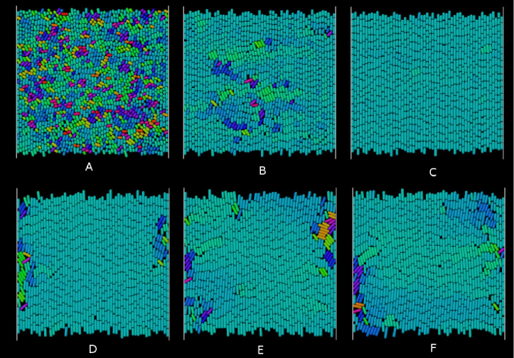
Figure 1: (Color online) Typical configurations of simulated bacterial colonies filling the channel, with the rods colored according to their orientation. A-C: Systems of low drag friction ($\mu=10^{-6}$) and different rod aspect ratio: $\ell_{0}=2.0$ (A), $\ell_{0}=3.0$ (B) and $\ell_{0}=4.0$ (C). The growth rate is $a=1.0$. Systems of longer rods have higher nematic order. D-F: Systems with $\ell_{0}=4.0$ and of varying drag friction: $\mu=0.45$ (D), $\mu=0.50$ (E) and $\mu=0.55$ (F), where disordered regions appear intermittently.

In this paper, inspired by experiments performed with a non-motile strain of E. coli bacteria (division time $\sim 20$ min) in microfluidic devices volfsonpnas , we perform molecular dynamics simulations of a system of growing and dividing rods with repulsive interactions. This system is confined by the lateral walls of a two-dimensional channel of finite length and open at both ends, where the particles can exit the channel. In the microfluidic experiments, the channel was limited in the third dimension by two walls whose separation distance was barely larger than the diameter of one bacteria. Therefore, although the rods are three-dimensional objects in the model, they form a single layer and their motion is assumed to be two-dimensional.

As shown by continuum theories of self-propelled particles baskaranprl2008 ; bartolo , the effect of boundaries and confinement have a strong impact on the ordering of active flows, where, for instance, the presence of the walls can induce a non-zero polarization. Similarly here, non-motile elongated particles push each other while they grow and tend to align parallel to the walls of the channel. In the long time regime, the rods that flow out of the channel are constantly replaced by new rods which form a dense model tissue inside the channel, with relatively small local density fluctuations volfsonpnas . In ref. physbiol , it was shown with the use of a phenomenological continuum theory and discrete element simulations that the perfectly ordered active nematic state was unstable with respect to small perturbations when a friction parameter exceeded a threshold value. This instability is analogous to a buckling instability and provokes the growth of the angles between the rods and the channel axis, allowing the release of the high compressive stresses generated by fully ordered configurations.

The aim of the present study is to investigate numerically the partially disordered states formed by these confined proliferating systems in the long time regime, when the statistical properties of the flow do not depend on time. We first quantify the effects on nematic ordering of the rod aspect ratio and of the friction that opposes rod motion. We then show that the nematic order parameter exhibits intermittent dynamics at intermediate frictions. We next focus on how the diagonal stress components fluctuate in time and space. We find that configurations subjected to larger longitudinal stresses are more ordered on average, whereas, locally, the distribution of contact forces is very heterogeneous and follows a power-law distribution in most cases.

II Model description

In our approach, thermal noise is neglected and rod dynamics is essentially deterministic. The discrete element soft-particle model used in this paper was described in previous works (see, e.g., volfsonpnas and physbiol ). Briefly, each cell is represented as a rigid rod consisting of a cylinder of fixed diameter set to unity for convenience and of two hemispherical caps at its ends. The length $l(t)$ of a given rod grows exponentially at a certain rate $a_{g}$ and the rod divides in two collinear rods of equal lengths when $l(t)$ reaches an assigned maximal length, denoted as $\ell_{m}$. To avoid spurious synchronization of cell divisions across the population, the division length $\ell_{m}$ is chosen randomly at the birth of each cell from a narrow normal distribution centered at a certain value $2\ell_{0}$ and with standard deviation $0.2\times 2\ell_{0}$. Similarly, $a_{g}$ is chosen from a distribution centered at a value $a$ and with standard deviation $0.1a$. Therefore, $a$ represents the mean growth rate of the rods in the system and $l_{0}$ the mean rod length at birth.

The rods are confined in a channel composed of two parallel walls separated by a distance $L_{x}$ (the transversal unit vector is denoted as $\hat{x}$) and length $L_{z}\equiv 2L$ (the longitudinal unit vector is denoted as $\hat{z}$). We set $L_{x}=L_{z}=55$ in the following. The rods cannot form more than one layer in the $\hat{y}$ direction, therefore motion is bidimensional. The channel boundaries at $z=\pm L$ are open: when the center of mass of a rod crosses one of the boundaries, the rod is removed from the system.

The normal contact forces between rods are obtained with the Hertzian model applied to the overlap of virtual spheres centered at the nearest points on the axes of interacting spherocylinders; similarly, the tangential (frictional) forces are given by the dynamic Coulomb friction ($\nu_{cc}$ is the coefficient of friction between cells) volfsonkudrolli . The microscopic parameters characterizing the elastic and dissipative properties of the cells coincide (unless indicated) with the ones used in volfsonpnas ; physbiol . In the experiments of ref.volfsonpnas , each cell is also subjected to forces due to the surrounding fluid and to the horizontal walls of the microfluidic chamber. These forces are modeled here by a Stokian drag force:

$${\mathbf{F}}^{(i)}_{f}=-\mu m^{(i)}{\mathbf{v}}^{(i)},$$ (1)

with ${\mathbf{v}}^{(i)}$ and $m^{(i)}$ the velocity and mass of rod $i$, respectively, and $\mu$ a drag friction constant. The contact and friction forces above are then used to compute the motion of each rod by integrating Newton’s equations.

For systems of rods that are perfectly oriented along the $z$ direction, simple continuum arguments predict that the flow is expansive and the pressure parabolic along the channel volfsonpnas : Assuming that the system reaches a steady state with constant rod density (while new rods are created, others exit the channel), the continuity equation reads ${\mathbf{\nabla}}\cdot{\mathbf{v}}=a$ and can be integrated as $v^{(0)}_{z}(z)=az$ and $v^{(0)}_{x}=0$. In the overdamped limit, the momentum conservation equation reads ${\mathbf{\nabla}}\cdot\sigma-\mu{\mathbf{v}}=0$, where $\sigma$ is the stress tensor. Imposing the boundary condition $\sigma=0$ at $z=\pm L$, one deduces that:

$$\sigma^{(0)}_{zz}(z)=\frac{1}{2}\mu a(z^{2}-L^{2}).$$ (2)

Hence, in response to the necessary growth of the rods the pressure adopts a parabolic profile and is maximal at the center of the channel ($z=0$), where $v_{z}$ vanishes. As illustrated by Eq. (2), varying the parameter $\mu$ allows to vary the magnitude of the average compressive load in the system.

III Behavior of the nematic order parameter

We simulated growing colonies starting from a few randomly oriented rods distributed in the channel. At large times, the density is roughly constant over time and the channel is filled with approximately 1000 rods in the examples of Figure 1. To measure the degree of alignment of the rods we calculated the scalar nematic order parameter:

$$Q=\overline{[\langle\text{cos}\ 2\phi\rangle^{2}+\langle\text{sin}\ 2\phi\rangle^{2}]^{1/2}},$$ (3)

where $\phi$ is the angle between the rod axis and some reference axis (the channel axis $\hat{z}$). The brackets above denote averages over all rods (spatial averaging) and the overbar, temporal averaging. In other words, $Q/2$ is the time average of the largest eigenvalue of the tensor order parameter in two dimensions, $\langle u_{\alpha}u_{\beta}-\frac{1}{2}\delta_{\alpha\beta}\rangle$, where the $u_{\alpha}$’s are the components of the orientational unit vector of a rod doiedwards . When the colony is in the disordered state $Q$ is close to zero, while perfect nematic order corresponds to $Q=1$.

III.1 Effects of rod shape and of friction

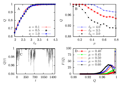
Figure 2: (Color online) A: Mean order parameter $Q$ as a function of the mean length of the rods at division ($\mu=0$, $\nu_{cc}=0$). The growth rate $a$ has a little impact on $Q$, as shown by the 3 overlapping curves. B: Mean order parameter $Q$ as a function of $\mu$ for different mean rod length ($\nu_{cc}=0$). C: A time series $Q(t)$ showing intermittent behavior at $\mu=0.45$, $\ell_{0}=4$. D: Probability distribution function of the global order parameter $Q(t)$ for different friction coefficients $\mu$. As $\mu$ increases, the most probable $Q(t)$ takes lower values.

We first consider systems with vanishing frictions ($\mu=0$, $\nu_{cc}=0$) and vary $\ell_{0}$ (Figures 1A-C). Even in this case where stresses are very small, the system may not be able to order perfectly. Figure 2A shows the nematic order parameter as a function of $\ell_{0}$. It is observed that for $\ell_{0}>3$ perfect nematic order is reached, whereas it decays rapidly if $\ell_{0}<3$. In systems of short rods (e.g., $\ell_{0}=2$, Fig. 1A) many disoriented regions are present and persist over time (see animation in SI ). It is worth noting that many bacteria such as E. coli have aspect ratio larger than $3$ turb2 and may therefore be prone to form dense ordered colonies in the presence of boundaries. The growth rate, on the other hand, has little impact on $Q$ in the asymptotic regime, as the three curves with $a=0.1,0.5$ and $1.0$ collapse onto each other in figure 2A.

When the friction $\mu$ is finite, nematic order can be significantly lower than in the case $\mu=0$, even for colonies of long rods ($\ell_{0}\geq 3$). As shown by Figure 1, the ordered states are roughly composed of flowing columns of rods parallel to each other. A larger friction should increase the pressure $-\sigma_{zz}$ exerted along the channel axis and thus increase the repulsive interaction forces between neighboring rods of a same column. According to the continuum analysis presented in physbiol this compressive energy can be released if the columns of rods bend (or buckle), producing less ordered configurations ($Q<1$). As expected from this scenario, we observe that $Q$ decays with $\mu$ (Figure 2B). For a fixed $\mu$, systems with larger $\ell_{0}$ are more ordered. This is also in qualitative agreement with the prediction of physbiol , where the bending constant $\xi$ in the elastic free energy of the system was estimated from the overlap of a rod with the rods of the neighboring columns, leading to $\xi\propto\ell_{0}^{3}$.

In all the following, we fix $\ell_{0}=4$. Figure 2C shows a typical time evolution of the order parameter $Q(t)$, obtained by taking the space average only, at relatively high friction ($\mu=0.45$). The colony can exhibit long periods of high nematic order, interrupted once in a while by bursts of disorder or “turbulence” (see animation in SI ). This intermittent behavior of $Q(t)$ is observed in a relatively narrow range of frictions, $\mu=0.40-0.50$.

III.2 Intermittent dynamics

Following a method similar to that proposed in ref. huepealdana to characterize the intermittent dynamics of an ordered active system, we extract from the corresponding time series the probability distribution function of $Q(t)$, for different values of the friction drag. As shown by Figure 2D, with $\mu=0.4$ (or lower) the distribution of $Q(t)$ is very peaked near unity, whereas with $\mu=0.6$ (or larger), completely ordered configurations are never reached during a typical simulation time. In the latter high friction range, the distribution has a most probable value $<1$ and a larger variance. There is an intermediate regime, roughly in the range $\mu\in[0.4,0.6]$, where the distribution is peaked at $Q=1$ and also has a second local maximum at some value $Q_{max}<1$. We thus consider in this regime that, at any given time, the system can be either in an “ordered” or in a “disordered” phase, depending whether $Q(t)>Q^{\ast}$ or $Q(t)<Q^{\ast}$, respectively, where $Q^{\ast}$ is a crossover value. Here we choose $Q^{\ast}$ as given by the secondary maximum $Q_{max}$ of the distribution. The results are not very sensitive to other choices of $Q^{\ast}$.

In this intermediate friction range, we can thus define a ordered (or “laminar”) time interval pomeau as the duration $\tau_{Q}$ separating two consecutive disordered episodes. To measure these durations, we record the time periods during which $Q(t)$ remains larger than $Q^{\ast}$ without interruption. The probability distribution function (p.d.f.) of $\tau_{Q}$ is shown in Figure 3 and exhibits a clear inverse power-law behavior over 3 decades, $F(\tau_{Q})\sim\tau_{Q}^{-\beta}$. The typical value of $\beta$ is 1.2 and depends little on $\mu$.

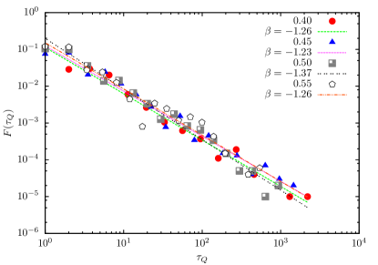
Figure 3: (Color online) Probability distribution function (p.d.f.) for the duration $\tau_{Q}$ of the laminar periods, with $\mu=0.45-0.55$. All curves show an inverse power-law behavior. The lines are best fits to the data, with their respective exponent estimates.

IV Pressure fluctuations

We next monitor the virial stress tensor caused by pairwise interactions between rods and defined as

$$\sigma_{\alpha\beta}({\mathbf{r}},t)=\frac{1}{2\mathcal{V}}\sum_{c,i}r_{\alpha}^{ic}F_{\beta}^{ic},$$ (4)

where ${\bf r}^{ic}$ is a vector from the center of mass of the rod $i$ to a point of contact with another rod, the index $i$ runs over all rods in a small mesoscopic volume $\mathcal{V}$ around the position ${\mathbf{r}}$; the index $c$ runs over all points of contacts.

IV.1 Global fluctuations

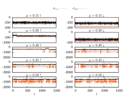
Figure 4: (Color online) Time evolution of the spatially averaged stress tensor components $\langle\sigma_{xx}\rangle(t)$ (continuous orange - gray - line) and $\langle\sigma_{zz}\rangle(t)$ (dotted black line) for different values of $\mu$ during a cycle. Left panel: System with increasing friction ($\uparrow$ branch). Right panel: System with decreasing friction ($\downarrow$ branch).

To study the temporal fluctuations of the stresses in the system as a whole, we consider the spatially averaged stress:

$$\langle\sigma_{\alpha\beta}\rangle(t)=\langle\sigma_{\alpha\beta}({\mathbf{r}},t)\rangle.$$ (5)

Typical time series of $\langle\sigma_{xx}\rangle=-\langle P_{x}\rangle$ and $\langle\sigma_{zz}\rangle=-\langle P_{z}\rangle$ for different values of $\mu$ are shown in Figure 4. In order to investigate possible hysteresis effects, we varied $\mu$ cyclically in a same simulation. In the left panel of Fig. 4, a system is prepared with $\mu=0.1$ and evolves during 1500 time units. The friction is then incremented of $0.05$ and kept constant for another 1500 time units. The procedure is repeated up to $\mu=0.80$ (“$\uparrow$” branch). From there, the friction is decreased in a similar way with decrements of $0.05$ down to $0.1$ again (“$\downarrow$” branch, right panel of Figure 4).

The spatially averaged pressure in the longitudinal direction, $\langle\sigma_{zz}\rangle(t)$, fluctuates little in time and does not show clear signs of hysteresis (see also the lower panel of Fig. 6). However, the pressure in the direction transverse to the channel axis, $\langle\sigma_{xx}\rangle(t)$, exhibits much larger temporal variations (orange - gray - curves of Fig.4). In Fig. 4, for $\mu=0.30$ and $0.40$ in the $\uparrow$ branch, for instance, one observes step-like variations or abrupt jumps occurring at random times between different stationary values. The average pressure in the $\hat{x}$ direction can vary in time by a factor of $\sim 7$ in a same dynamics.

As shown by Figure 5, these practically discrete jumps in the transversal pressure are due to the rapid formation (or elimination) of one or more columns of rods, which are oriented along the $\hat{z}$ direction. The number of rod columns exhibits a similar step-like dynamics. As a new rod column appears, the system becomes more crowded in the $\hat{x}$ direction, resulting in a sharp increase in $|\langle\sigma_{xx}\rangle|$. On the contrary, when a column disappears, the pressure is relaxed.

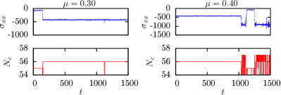
Figure 5: (Color online) The spatially averaged stress tensor component $\langle\sigma_{xx}\rangle(t)$ (upper panels) at a given time is closely related to the number $N_{c}$ of rod columns that fill the channel at the same time in the transverse direction (lower panels).

Higher frictions cause an increase in both $P_{x}$ and $P_{z}$ on average (see Fig. 6). The increase of $P_{z}$ with $\mu$ is due to the higher friction forces exerted on the particles, has qualitatively predicted by Eq. (2). The increase in $P_{x}$ is due to the fact that at higher frictions the system tends to form more columns and thus denser populations along the $\hat{x}$ direction. This densification was already noticed right after the buckling instability in ref. physbiol . If the friction is further decreased, the high transverse densities may persist. For this reason, at the end of the hysteresis loop ($\mu=0.15\downarrow$, Fig. 4) the transverse pressure can be much higher than what it was at the beginning ($\mu=0.15\uparrow$). The higher panel of Figure 6 illustrates the hysteretic behavior of the time averaged pressure $|\overline{\langle\sigma_{xx}\rangle}|$. Note that at the beginning of the loop the time intervals between jumps can be large and thus the time averages may vary from one simulation to another due to the limited observation time.

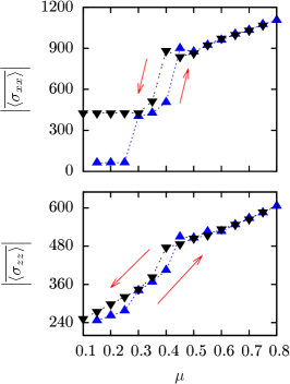
Figure 6: (Color online) Time averages $\overline{\langle\sigma_{xx}\rangle}$ and $\overline{\langle\sigma_{zz}\rangle}$ of the spatially averaged stress tensor components. The $\uparrow$ and $\downarrow$ branches of the cycle are labeled with blue up-triangles and black down-triangles, respectively.

IV.2 Distribution of local stresses

To examine how the local pressure fluctuates in space and time, we display in Figure 7 the probability distribution functions of the local stresses $P_{x}$ and $P_{z}$, given by Eq. (4). These p.d.f’s are obtained by aggregating all positions and times of a given simulation.

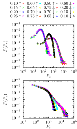
Figure 7: (Color online) Probability distribution function of the local pressure for different values of $\mu$, which is varied cyclically: $\mu=0.1\rightarrow 0.8\rightarrow 0.1$. For clarity, only the cases $\mu\leq 0.25$ and $\mu\geq 0.60$ are shown. Upper panel: Distributions of $P_{x}$, where the curves for $\mu\leq 0.25$ ($\uparrow$), $\mu\geq 0.60$ ($\uparrow$ and $\downarrow$) and $\mu\leq 0.25$ ($\downarrow$) are located on the left part, right part and middle part of the graph, respectively. Lower panel: Distributions of $P_{z}$, where the curves with broader tails correspond to $\mu\geq 0.60$.

The hysteresis effects observed above on $\langle\sigma_{xx}\rangle$, are noticeable in the full distribution, which has a characteristic scale given by its most probable value. In the $\uparrow$ branch, the most probable values of $-\sigma_{xx}$ for $\mu\leq 0.25$ are much lower than the most probable values for $\mu\geq 0.60$. When low friction values ($\mu\leq 0.25$) are reached again in the $\downarrow$ branch, the most probable $-\sigma_{xx}$ returns to a value larger than its initial value (middle curves of Figure 7, upper panel).

The distribution of $P_{z}$, shown in Figure 7, lower panel, does not exhibit such hysteresis and has a markedly different shape: it is monotonic decreasing and independent of $\mu$ at small $P_{z}$. In this regime, the distribution is approximately scale-free, i.e., well described by a power-law with exponent $\approx-0.7$. Hence, the gradual increase of the average longitudinal stress produced by increasing $\mu$ (see Fig. 6) does not modify much how stresses are distributed locally among the rods: it only produces a broadening of the tail of the distribution. Many regions carry small stresses and contribute little to the average pressure, even at high $\mu$, whereas a few rare places have stresses much higher than average. Therefore, the longitudinal pressure field is very heterogeneous in space and time. For $\mu\leq 0.25$, a fit shows that the distribution decays exponentially at very large $P_{z}$. However, for $\mu\geq 0.60$, the tail of the distribution is better described by a second power-law, with steeper exponent $\approx-2$.

For comparison, it is instructive to calculate the p.d.f $F^{(0)}(P_{z})$ predicted by the continuum theory where the rods are assumed to be perfectly aligned and where $P_{z}(\mathbf{r},t)$ is stationary and only depends on $z$. From the parabolic profile given by Eq.(2) and from the general property $|F^{(0)}(P)dP|=|g(z)dz|$, where $g(z)$ is the distribution of $z$ ($g(z)=cst$ along the channel), one obtains:

$$F^{(0)}(P_{z})\propto\frac{1}{(1-P_{z}/P_{0})^{1/2}}.$$ (6)

According to this result, elementary regions of space where the pressure is larger (close to the maximum $P_{0}$, at the center of the channel) should be more frequent than regions with lower pressures. Such behavior is opposite to that of the distributions of Figure 7 (lower panel). This result illustrates that local disorder profoundly reorganizes the system by a redistribution of stresses. This situation is reminiscent of the heterogeneous distributions of contact forces in static granular systems. Nevertheless, contact force distributions are exponential in static systems and thus have a typical scale forcefluct .

IV.3 Correlations with $Q$

Figure 8: (Color online) Parametric plots $Q(t)$ vs. $\langle\sigma_{xx}\rangle(t)$ and $Q(t)$ vs. $\langle\sigma_{zz}\rangle(t)$ at $\mu=0.50$.

To investigate the interplay between nematic order and pressure at a given time, we calculated the Pearson correlation coefficients between $Q(t)$ and $\langle\sigma_{xx(zz)}\rangle(t)$. Given two arbitrary discrete time series $a_{i}$ and $b_{i}$ of means $\overline{a}$ and $\overline{b}$, respectively, this coefficient is defined as

$$\rho_{ab}=\frac{\sum_{i=1}^{n}(a_{i}-\overline{a})(b_{i}-\overline{b})}{\sqrt{\sum_{i=1}^{n}(a_{i}-\overline{a})^{2}}\sqrt{\sum_{i=1}^{n}(b_{i}-\overline{b})^{2}}}.$$ (7)

The cases $\rho_{ab}=1$, $-1$ and $0$ correspond to perfectly correlated, anti-correlated and not correlated variables, respectively. In Figure 8, each dot represents a particular time step of a dynamics.

Table 1 shows that $Q(t)$ tends to be significantly anti-correlated to $\langle\sigma_{zz}\rangle(t)$, independently of $\mu$. This property indicates that, at a given time, a more ordered configuration is likely to be subjected to larger longitudinal stresses. This finding is consistent with the fact that gradients in the rod orientations (mis-alignments) actually release the compressive longitudinal energy physbiol .

To check whether there exists a relationship between the step-like variations of $\langle\sigma_{xx}\rangle(t)$ at intermediate frictions (see Figure 4) and the intermittent dynamics of $Q(t)$ observed in about the same friction range, we calculated the Pearson coefficient between (i) $Q(t)$ and $\langle\sigma_{xx}\rangle(t)$, (ii) $Q(t)$ and $|d\langle\sigma_{xx}\rangle(t)/dt|$ and (iii) $|dQ(t)/dt|$ and $|d\langle\sigma_{xx}(t)\rangle/dt|$. As shown by Table 1, very weak correlations are found in almost all cases. Therefore, there seems to be no systematic correlations between the fast variations in $\langle\sigma_{xx}\rangle(t)$ and the intermittent bursts of nematic disorder, except maybe for lower frictions, see $\mu=0.4$ and $0.45$ in Table 1. This suggests that the mechanisms by with the system modulates its transversal pressure under confinement (through the formation or elimination of columns of growing rods) is not directly related to the ordering dynamics itself. The mis-alignment of some rods does not preferentially leads to a lower transverse pressure, contrary to what happens in the longitudinal direction.

$\mu$	$Q\ \&\ \sigma_{zz}$	$Q\ \&\ \sigma_{xx}$	$Q\ \&\ |\dot{\sigma}_{xx}|$	$\dot{Q}\ \&\ |\dot{\sigma}_{xx}|$
0.40	-0.27	-0.17	-0.03	$\sim 0$
0.45	-0.38	-0.20	0.03	$\sim 0$
0.50	-0.34	0.04	-0.01	$\sim 0$
0.55	-0.34	0.04	-0.00	$\sim 0$

Table 1: Numerical values for the Pearson correlation coefficient from time series where $Q(t)$ has an intermittent behavior. These values correspond to the $\downarrow$ part of the cycle (similar values are found for the $\uparrow$ part).

V Conclusions

We have studied with molecular dynamics simulations the ordering of systems of growing elongated particles confined in a channel. We find that the average nematic order parameter depends crucially on the rod aspect ratio, a parameter which is difficult to incorporate in continuum theories. Colonies fail to order parallel to the side walls if $\ell_{0}<3$, even when the drag friction is vanishing. For $\ell_{0}>3$ and at finite friction, intermittent bursts of disorder can take place and the periods during which the system remains well-ordered are power-law distributed. In another context, intermittent dynamics for the global order parameter have already been observed in active systems of self-propelled particles governed by the Vicsek model rules huepealdana .

Our results also show that the stress tensor is very anisotropic and that the pressure field has markedly different properties in the directions transverse and longitudinal to the channel axis ($\hat{x}$ and $\hat{z}$, respectively). Whereas $P_{x}$ is relatively homogeneously distributed in space, its spatial average can vary very rapidly in time due to stochastic and abrupt density variations in the lateral direction. This density can remain constant for long periods of time at low friction, which leads to hysteresis effects ohta . The fast variations of the spatial average $\langle P_{x}\rangle(t)$ at intermediate frictions do not seem to be correlated to the intermittent dynamics of the nematic order parameter. Comparatively, the spatially averaged $\langle P_{z}\rangle(t)$ has a much smoother behavior in time and does not present hysteresis, but it is correlated to the global nematic order parameter. This is to be expected from theoretical arguments that predict that longitudinal stresses should be released in systems of misaligned rods physbiol .

We emphasize that, unlike $P_{x}$, the longitudinal pressure $P_{z}$ is very heterogeneously distributed in space, in such a way that most of the rods are subjected to small stresses while very large stresses are supported by a few rods. This trend is opposite to the prediction of a simple continuum theory (that ignores granularity), which is that not-so-stressed rods should be less numerous than highly stressed rods. The distribution of $P_{z}$ is well fitted by a truncated power-law at low friction and by two power-laws at large friction. For comparison, the probability distribution function of the contact forces in jammed packings of non-active grains is generically exponential, i.e. comparatively much more homogeneous forcefluct . Contact forces also remain exponentially distributed in sheared packings of elongated particles azema .

In the proliferating systems studied here, a global state of compressive stress thus emerges from individual cell growth and division. This parallels the case of advancing sheets of epithelial cells in a channel, where global states of tensile stress have been observed in experiments nphys2010 . In those experiments, traction did not result from leader cells at the edge of the sheet dragging those behind, but from the cells located deep inside the tissue. It was observed that the traction force also followed a profile approximately parabolic, and exhibited, at a fixed location, large temporal fluctuations. These fluctuations were exponentially distributed, though, as in static granular materials nphys2010 .

Previous studies have shown that dense colonies of growing bacteria are able to self-organize and form crowds that efficiently escape from confining domains groisman . Our results further suggests that active systems subjected to external perturbations (such as an average pressure increase) could have the ability to self-organize in such a way that only a few particles would actually be affected by the perturbation. Our findings could have implications for understanding the growth of real tissues and biofilms, where individual cells subjected to large stresses are known to grow at a reduced rate or not to grow at all tumorjtb ; volfsonpnas . Colonies of bacteria or other cell types may be able to keep growing in adverse conditions and the study of such robustness should motivate further studies.

- (1) X.-L. Wu and A. Libchaber, Phys. Rev. Lett. 84, 3017 (2000).
- (2) T. S. Deisboeck and I. D. Couzin, BioEssays 31, 190 (2009).
- (3) A. Kudrolli, G. Lumay, D. Volfson, and L. S. Tsimring, Phys. Rev. Lett. 100, 058001 (2008).
- (4) M.C. Marchetti, J.F. Joanny, S. Ramaswamy, T.B. Liverpool, J. Prost, Madan Rao, and R. Aditi Simha, arXiv:1207.2929 [cond-mat.soft] (2012).
- (5) H. H. Wensink and H. Lwen, J. Phys.: Condens. Matter 24, 464130 (2012).
- (6) H. H. Wensink, J. Dunkel, S. Heidenreich, K. Drescher, R. E. Goldstein, and J. M. Yeomans, Proc. Natl. Acad. Sci. USA 109, 14308 (2012).
- (7) J. Dunkel, S. Heidenreich, K. Drescher, H. H. Wensink, M. Bar, and R. E. Goldstein, Phys. Rev. Lett. 110, 228102 (2013).
- (8) S. Henkes, Y. Fily, and M. C. Marchetti, Phys. Rev. E 84, 040301(R) (2011).
- (9) H. P. Zhang, A. Be’er, E.-L. Florin, and H. L. Swinney, Proc. Natl. Acad. Sci. USA 107, 13626 (2010).
- (10) F. Peruani, J. Starruß, V. Jakovljevic, L. Søgaard-Andersen, A. Deutsch, and Markus Bar, Phys. Rev. Lett. 108, 098102 (2012).
- (11) Y. Yang, V. Marceau, and G. Gompper, Phys. Rev. E 82, 031904 2010.
- (12) R. D. Campbell, J. Morphol. 121, 19 (1967).
- (13) G. Cheng, B. B. Youssef, P. Markenscoff, and K. Zygourakis, Biophys. J. 90, 713 (2006).
- (14) M. Poujade, E. Grasland-Mongrain, A. Hertzog, J. Jouanneau, P. Chavrier, B. Ladoux, A. Buguin, and P. Silberzan, Proc. Natl. Acad. Sci. USA 104, 15988 (2007).
- (15) A. R. Kansal, S. Torquato, G. R. Harsh, E. A. Chiocca, and T. S. Deisboeck, J. Theor. Biol. 203, 367 (2000).
- (16) A. Baskaran and M. C. Marchetti, Phys. Rev. Lett. 101, 268101 (2008).
- (17) A. Baskaran and M. C. Marchetti, Phys. Rev. E 77, 011920 (2008).
- (18) F. Ginelli, F. Peruani, M. Br, and H. Chaté, Phys. Rev. Lett. 104, 184502 (2010).
- (19) A. Peshkov, I. S. Aranson, E. Bertin, H. Chaté, and F. Ginelli, Phys. Rev. Lett. 109, 268701 (2012).
- (20) T. Brotto, J.-B. Caussin, E. Lauga, and D. Bartolo, Phys. Rev. Lett. 110, 038101 (2013).
- (21) D. Volfson, S. Cookson, J. Hasty, and L. S. Tsimring, Proc. Natl. Acad. Sci. USA 105, 15346 (2008).
- (22) D. Boyer, W. Mather, O. Mondragón-Palomino, S. Orozco-Fuentes, T. Danino, J. Hasty, and L. S. Tsimring, Phys. Biol. 8, 026008 (2011).
- (23) D. Volfson, A. Kudrolli, and L. S. Tsimring, Phys. Rev. E 70, 051312 (2004).
- (24) H. Cho, H. Jnsson, K. Campbell, P. Melke, J. W. Williams, B. Jedynak, A. M. Stevens, A. Groisman, A. Levchenko, PLoS Biol. 5, e302 (2007).
- (25) M. Doi and S. F. Edwards,The theory of polymer dynamics (Oxford University Press, Oxford, 1986).
- (26) Supplemental Material files.
- (27) C. Huepe and M. Aldana, Phys. Rev. Lett. 92, 168701 (2004).
- (28) P. Berge, Y. Pomeau, and C. Vidal, Order Within Chaos: Towards a Deterministic Approach to Turbulence (John Wiley and Sons, Inc., New York, 1987).
- (29) C.-h. Liu, S. R. Nagel, D. A. Schecter, S. N. Coppersmith, S. Majumdar, O. Narayan, and T. A. Witten, Science 269, 513 (1995).
- (30) E. Azéma and F. Radja, Phys. Rev. E 85, 031303 (2012).
- (31) Hysteresis behavior is also found in (non-confined) systems of deformable self-propelled particles with repulsive interactions, see Y. Itino, T. Ohkuma, and T. Ohta, J. Phys. Soc. Jpn. 80, 033001 (2011).
- (32) X. Trepat, M. R. Wasserman, T. E. Angelini, E. Millet, D. A. Weitz, J. P. Butler, and J. J. Fredberg, Nature Phys. 5, 426 (2010).