Toward a Deterministic Model of Planetary Formation VII:
Eccentricity Distribution of Gas Giants

Abstract

The ubiquity of planets and diversity of planetary systems reveal planet formation encompass many complex and competing processes. In this series of papers, we develop and upgrade a population synthesis model as a tool to identify the dominant physical effects and to calibrate the range of physical conditions. Recent planet searches leads to the discovery of many multiple-planet systems. Any theoretical models of their origins must take into account dynamical interaction between emerging protoplanets. Here, we introduce a prescription to approximate the close encounters between multiple planets. We apply this method to simulate the growth, migration, and dynamical interaction of planetary systems. Our models show that in relatively massive disks, several gas giants and rocky/icy planets emerge, migrate, and undergo dynamical instability. Secular perturbation between planets leads to orbital crossings, eccentricity excitation, and planetary ejection. In disks with modest masses, two or less gas giants form with multiple super-Earths. Orbital stability in these systems is generally maintained and they retain the kinematic structure after gas in their natal disks is depleted. These results reproduce the observed planetary mass-eccentricity and semimajor axis-eccentricity correlations. They also suggest that emerging gas giants can scatter residual cores to the outer disk regions. Subsequent in situ gas accretion onto these cores can lead to the formation of distant ($\gtrsim 30$AU) gas giants with nearly circular orbits.

1 Introduction

The accelerating pace of observational discovery (with radial velocity, transit, microlensing, and direct imaging surveys) provide rich data sets on the statistical properties of extra solar planets and planetary systems. In order to extract, from these data, useful information on the dominant physical processes and appropriate range of physical condition associated with planetary formation and evolution, population synthesis models have been developed. In a series of papers (Ida & Lin, 2004a, b, 2005, 2008a, 2008b, referred to as Paper I-V), we and others (Mordasini et al., 2009a, b; Alibert et al., 2011) have outlined prescriptions for various physical processes and described attempts to reproduce observational data with simulated models. Some of the relevant effects have been taken into account so far include the coagulation of planetesimals into embryos, gas accretion onto sufficiently massive cores, type I and II migration of individual protoplanets due to their interaction with their natal disks.

Recent transit search by the Kepler space telescope indicates that many, if not most, super-Earths have siblings, i.e., they are members of multiple-planet systems. In these systems, gravitational interaction between planets affects not only the formation but also their evolution and destiny. There have been several attempts to describe the dynamical evolution of these systems with N-body simulations. Due to the time consuming nature of such approaches, only limited range of initial parameters have been explored. It is not clear whether these models adequately represent the distribution of multiple planet systems.

The population synthesis method is based on a statistical mechanics approach to evaluate the most likely outcome of dynamical interactions between planets. In order to describe the statistical outcome of gravitational interactions and collisions between rocky planetary embryos, we have upgraded our population synthesis method to generate a series of many simulations. In paper VI (Ida & Lin, 2010), we described our analytic prescription for the collisions and close scatterings between modest-mass planets. We applied this method to show that super-Earths may be the in situ merger products of a population of embryos with Earth-mass or less which converged towards the proximity of their host stars through type I migration.

Radial velocity survey show that modest to long-period ($>7-10$ days) gas giants also have significant eccentricity. These planets most likely have formed in their natal disks with nearly circular orbits as in the case of Jupiter and Saturn (Pollack et al 1996, Ida & Lin 2004). Their eccentricity may have been excited by the gravitational perturbation of their planetary siblings (Rasio & Ford 1996, Zhou et al 2007, Jaric & Tremaine 2008, Chatterjie et al 2008). Indeed, many gas giant planets are members of known multiple-planet systems.

In order to simulate the outcome of dynamical interaction between gas giants and their siblings including other gas giants as well as less-massive protoplanetary embryos, we construct in this paper, construct a ”multiple-planet-in-a-disk model”. This approach is a natural continuation of the method presented in Paper VI. The main technical challenge is that the gravitational perturbations from gas giants significantly affect orbital configuration of the entire planetary system.

The method we have developed to approximate the evolution of systems of N gas giants is presented in §2. This prescription takes into account gravitational interactions between all the planets around their common host stars. It reproduces the general results of direct N-body simulations with a large reduction (by many orders of magnitude) in the computational cost. A detailed description of the method is given in the Appendix.

We incorporate this prescription into the latest version of the population synthesis models. In §3, we briefly recapitulate the methodology used in our population synthesis models including prescriptions for: 1) disk structure and evolution, 2) planetesimal growth and the planetary embryos’ dynamical isolation, 3) migration due to tidal interaction between protoplanets and their natal disks, and 4) resonant interaction between protoplanets.

In §4, we apply these prescription to simulate some sample multiple-planet systems. These results show that that 1) the most favorable location for gas giant formation in the core-accretion scenario is at a few AU’s, 2) the emergence of gas giants leads to the scattering of residual protoplanetary embryos, some of which may subsequently undergo gas accretion and form later generation gas giants, 3) as a consequence of dynamical instability, some gas giants in multiple-planet systems may be scattered to attain the observed eccentricity distribution.

An advantage of the population synthesis model is its computational efficiency. With it, we are able simulate in §5 rich sets of planetary systems based on the observed range of disk properties. We compare the results obtained from the population synthesis models with the observational data. Our models reproduce the observed planetary mass - eccentricity and semimajor axis - eccentricity correlations. These comparisons are important not only to calibrate some uncertainties in the model parameters but also to highlight the dominant physical processes.

Finally in §6, we summarize our results and discuss their implications.

2 Modeling of eccentricity excitation and ejection of giant planets as a result of gravitational instability

The objective of this section is to introduce a simple-to-use and computationally-efficient prescription to approximate the dynamical interaction between multiple planets around common host stars.

2.1 An overview of our technical approach

Before outlining the technical details of our prescription, we first qualitatively describe the principles of our analytic approximation for the gravitational interactions between several gas giants. This approach is guided by the results generated from various N-body simulations of the dynamical interaction between giant planets. Many such simulations have been carried out for the purpose of studying the statistical properties associated with close encounters between multiple planets especially with regard to the origin of the eccentric as well as short-period Jupiter-mass planets (e.g. Rasio & Ford, 1996; Weidenschilling & Marzari, 1996; Ford et al., 2000; Zhou et al., 2007; Ford & Rasio, 2008; Jurić & Tremaine, 2008; Marzari & Weidenschilling, 2002; Nagasawa et al., 2008; Chatterjee et al., 2008).

Most of the N-body experiments have been carried out with idealized initial conditions. They show that 1) the onset of dynamical instability is sensitively determined by the planets’ initial normalized (in terms of their Hill’s radius) separation and 2) dynamically unstable systems undergo orbit crossing and relaxation which generally lead to a Rayleigh distribution in the planets’ asymptotic eccentricity (Ida & Makino, 1992; Zhou et al., 2007). In order to check the validity of our prescription (to be presented below), we perform calculations with our analytic prescriptions for the same initial conditions as those adopted by the previous N-body simulations.

There are some analytic approximation for the stability of planetary systems. Two planets with masses $m_{1}$ and $m_{2}$ on initially circular orbits around a common host star with a mass $M_{*}$ ($\gg m_{1},m_{2}$) would immediately cross each other’s path if the difference between their semimajor axes ($\Delta a$) is smaller than a critical value,

$$\Delta a_{\rm c}\simeq 2\sqrt{3}r_{\rm H}$$ (1)

where $a$ is the average of their semimajor axis and

$$r_{\rm H}=((m_{1}+m_{2})/3M_{\ast})^{1/3}a$$ (2)

is there mutual Hill’s radius. But, orbital crossings in such a system would not occur if initially $\Delta a$ is slightly larger than $\Delta a_{\rm c}$ (Gladman, 1993). In §2.2, we present a prescription to evaluate the asymptotic semimajor axis and eccentricity distributions of two-planet systems which undergo orbital crossings.

In systems with three or more gas giants, the orbit-crossing condition is significantly different. For a finite duration of time, systems with initial $\Delta a$ larger than $\Delta a_{\rm c}$ may be maintained in a quasi-stable state with a limited variation in the amplitude of eccentricity. However, in due course, such systems may undergo a transition with a rapid eccentricity increase which is followed by orbital crossings (Chambers et al., 1996; Lin & Ida, 1997; Marzari & Weidenschilling, 2002; Zhou et al., 2007). The time scale $\tau_{\rm cross}$ for the onset of this transition depends sensitively on the normalized initial orbital separation $\Delta a/r_{\rm H}$, the planet-to-star mass ratio, and weakly on the number of planets.

In the population synthesis model (see §3), we consider the possibility that the giant planets and rocky/icy planetary embryos may form, coexist, and evolve contemporaneously in a gaseous environment. During advanced stages of their formation, gas giants grow through runaway gas accretion, i.e., the time scale $\tau_{\rm KH}$ for them to double their mass $M_{p}$ decreases with $M_{p}$. Their Hill’s radius and the width of their feeding zone also increases with their $M_{p}$. The eccentricity of the nearby planetary siblings and residual embryos (with $\Delta a<\Delta a_{\rm c}$) would be excited over their synodic periods $\tau_{\rm syn}$ with respect to the orbits of the gas giants.

While multiple planets’ eccentricity is excited by their secular interaction with each other, it is also damped by their tidal interaction with their natal disks (Artymowicz, 1993; Ward, 1993; Tanaka & Ward, 2004). It is appropriate to take into account these competing effects (Iwasaki et al., 2002) (see §3). Planet-disk interaction also leads to type I and II migration (for modest-mass embryos and high-mass gas giants respectively). Idealized prescriptions for isolated planets’ migration have already been incorporated into early versions of population synthesis models (Papers I & V). In a subsequent paper, we will develop and apply a new prescriptions for embryos’ type I migration (Paardekooper et al., 2011) and consider the feedback on the disk structure by multiple gas giants and their interference on each other’s direction and speed of migration.

In this paper, we focus on dynamical interaction between multiple gas giants in the limit that the difference between their semimajor axis may be reduced during the course of their migration. Two gas giants would capture each other onto their mutual low-order mean-motion resonances provided the convergent speed is slow. This effect has already been analyzed with our population synthesis models for interaction between rocky and icy embryos (Paper VI). In §2.2, we modify our prescription to take into the nonlinear interaction and determine the resonant capture condition between multiple gas giants. We also consider the critical converging speed above which the gas giants may overcome the resonances’ barrier and intrude into each other’s Hill’s sphere and undergo close encounters (see §3.6).

The intensity of planet-disk interaction reduces with the depletion of the disk gas. Observational signatures of protostellar disks diminish on a time scale of 3-5 Myr. The accretion rate from the disk to the central stars (inferred from the UV veiling) also declines on a similar time scale (Hartmann, 1998). Our population synthesis models take into account disk evolution and adjust the effects of gas accretion, eccentricity damping, and orbital migration accordingly. After the disk gas is severely depleted, both gas damping and accretion cease while secular interaction between the planets persists.

In Paper VI, we presented prescriptions for eccentricity excitations and merging events (giant impacts) among the rocky/icy planetary embryos. For these relatively low-mass objects, we construct an analytic approximation to determine the outcome of the dynamical interaction between planets based on celestial mechanics. This prescription quantitatively reproduce the results of N-body simulations. We applied this prescription to simulate the evolution of systems of 10–20 embryos with a total mass of a few $M_{\oplus}$. This initial condition corresponds to the the advanced stage of oligarchic growth when the embryos become dynamically isolated. We showed that close encounters generally lead to a velocity dispersion $\sigma$ which is a significant fraction of the embryos’ surface escape speed. Within a few AU’s, embryos are unlikely to be ejected because $\sigma$ is smaller than the local Keplerian speed $v_{\rm K}$. After the gas depletion, repeated close encounters lead to mergers and the emergence of one or two Earth-mass planets with few residual embryos. Thereafter, the magnitude of $\tau_{\rm cross}$ increases beyond the main sequence life span of solar type stars (ie $10^{9}-10^{10}$ yrs). We also used this prescription to show that some super-Earths may be the merger products of a population of embryos which migrated to the proximity of their host stars.

In §2.3 of this paper, we generalize our prescription to simulate the onset of dynamical instability and resultant orbital crossings among multiple gas giants in the outer regions of an evolving disk environment. The recoil motion excites the eccentricity of the retained planets to establish a Rayleigh’s distribution similar to that observed among eccentric gas giants (Rasio & Ford, 1996; Weidenschilling & Marzari, 1996; Lin & Ida, 1997; Marzari & Weidenschilling, 2002). In contrast to the embryos close to their host stars, the surface escape speed of typical gas giants exceeds the Keplerian speed in the outer regions of their natal disks where they emerge. Close encounters with gas giants at few AU from the host stars may lead to ejection rather than merger events.

The crossing timescale $\tau_{\rm cross}$ increases with the semimajor axis separations and decreases with the orbital eccentricities. As the population of gas giants declines through merger and ejection events or migration and stellar consumption, their normalized semimajor axis separation ($\Delta a/r_{\rm H}$) is enlarged. Energy dissipation during cohesive collisions also leads to eccentricity damping. These combined effects lengthen $\tau_{\rm cross}$ by several orders of magnitude after each merger or ejection event.

Recent numerical simulations show that there is a $\sim 30\%$ chance for orbital crossings to eventually excite one of the gas giants to attain nearly parabolic orbit by Kozai effect (Nagasawa et al., 2008). The orbit of an inwardly scattered gas giant may be circularized if its pericenter distance is sufficiently close to the host star (Ivanov & Papaloizou, 2004). This scenario has been suggested as one of the mechanism for the origin of “hot Jupiters” (Rasio & Ford, 1996; Nagasawa et al., 2008). We have not incorporated tidal circularization and secular perturbations including the Kozai effect into the current version of the population synthesis models, although the overall effects of secular eccentricity excitation is implicitly taken into account through the assumption that the orbital crossings start on timescale $\tau_{\rm cross}$.

2.2 Two gas giants case

The above description qualitatively outlines the overall methodology of our population synthesis model. We now provide some technical details on its latest upgrade, i.e., the construction of an analytic plus Monte Carlo prescription.

We begin with the simplest case of dynamical interaction between two gas giants. As we have indicated above, in this case, orbit crossing are expected to occur between two planets with nearly circular co-planar orbits which are initially separated in semimajor axis by $\Delta a<\Delta a_{\rm c}$. Extensive numerical simulations show that close encounters between these planets generally leads to the expansion of their semimajor axis separation and eccentricity excitation. We construct a method to compute the outcome of these close encounters. This prescription is calibrated with the statistical results generated from numerical simulations (Ford et al., 2000; Ford & Rasio, 2008). Detailed prescriptions are described in the Appendix A1.

The procedure of our model for two-planet encounters is structured in the following manner.

A1)

We first identify two interacting gas giants, with mass $m_{1}$ and $m_{2}$.

A2)

We compute the maximum relative eccentricity attainable during a close scattering in terms of the two-body surface escape velocity ($v_{{\rm esc},12}$) scaled by the local Keplerian velocity ($v_{\rm K}$), such that,

$$e_{{\rm esc},12}=\frac{v_{{\rm esc},12}}{v_{\rm K}}\simeq 1.6\left(\frac{m_{1}+m_{2}}{M_{\rm J}}\right)^{1/3}\left(\frac{\rho}{1{\rm gcm}^{-3}}\right)^{1/6}\left(\frac{a}{1{\rm AU}}\right)^{1/2}.$$ (3)

A probable eccentricity is generated for individual bodies $j(j=1,2)$ with

$$e_{j}^{\rm max}=\left(\frac{m_{k}{\cal R}_{j}}{m_{1}+m_{2}}\right)e_{\rm esc,12},$$ (4)

where $k\neq j$ refers to the perturbing companios and

$${\cal R}_{j}(x,\sigma)=(x/\sigma^{2}){\rm exp}(-x^{2}/2\sigma^{2})$$ (5)

is a random number with a Rayleigh distribution of unit root mean square dispersion $\sigma$,

A3-a)

If, at least one of the trial eccentricities (given by Eq. 4) exceeds unity, the body with the larger eccentricity would be identified as a planet to be ejected. The remaining planet is assumed to be retained. For it, a new eccentricity is generated (with Eqs. 6 and 7) together with an associated semimajor axis (with Eq. 45) (see §2.2.1).

A3-b)

If the trial eccentricities of both planets are less than unity, they would be adopted as the expected values for the two planets after their close encounters with some damping (see step 3-b in Appendix A1). The associated semimajor axis changes are evaluated in accordance with the prescription in §2.2.2.

This procedure is applied throughout the disk evolution. Prior to severe gas depletion, the damping of eccentricity due to the planets’ tidal interaction with their natal disks is taken into account. The combined effect of planet-planet scattering and planet-disk tidal interaction induce the two planets to enlarge their semimajor axis separation $\Delta a$ until they become dynamically isolated with $\Delta a>\Delta a_{\rm c}$. The efficiency of gas damping declines during gas depletion. In the absence of any significant amount of residual disk gas, two planets with $\Delta a>\Delta a_{\rm c}$ would continue to scatter each other until either they merge with each other or one of them is ejected.

2.2.1 Planetary escape after close encounters between two planets

We consider the possibility that one member of a planet pair may attain sufficient recoil velocity to escape from the gravitational potential of their host star. We compare the results generated with our analytic plus Monte Carlo prescription with those obtained from N-body simulations which were computed without taking into account of any eccentricity damping effect (due to either planet-disk interaction or dissipative collisions.).

Since both interacting planets were initially bound to their host stars, conservation of energy implies that at least one of them must be retained. We label the retained and ejected planets as body 1 and 2 respectively. In Appendix A1, we derived the differential distribution function of the post-scattering eccentricity of the retained body 1 as

$$f(e)de\propto\frac{1}{\sqrt{2\pi}(e^{*}/3)}\exp\left(-\frac{(e-e^{*})^{2}}{2(e^{*}/3)^{2}}\right)de,$$ (6)

where

$$e^{*}=0.83\frac{m_{2}}{m_{1}}-0.17\left(\frac{m_{2}}{m_{1}}\right)^{2},$$ (7)

and $m_{1}$ and $m_{2}$ are masses of retained and ejected planets respectively. Since it takes less energy to eject the lighter body, we assume $m_{1}>m_{2}$ which is also consistent with the results of N-body simulations.

In Eqs. (6) and (7), the eccentricity distribution function depends on the ratio rather than the individual values of $m_{1}$ and $m_{2}$. The results of numerical simulation of close encounters between two equal mass planets Ford & Rasio (2008) also show a negligible dependence of $\mu=m_{1}/M_{*}=m_{2}/M_{*}$ (in the range between $0.001-0.01$). Note from Eq. (3), ejection cannot be produced from close encounters between planets with $\mu\ll 10^{-4}(\rho/1{\rm gcm}^{-3})^{-1/2}(a/1{\rm AU})^{-3/2}$).

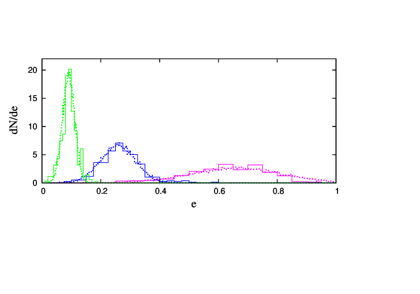
Figure 1: Dynamical instability and asymptotic properties of systems with two closely separated gas giant planets. All the models start with two planets with a total mass $(m_{1}+m_{2})/M_{*}=0.006$ around a common host star. Their initial orbits are nearly circular and coplanar with a unstable semimajor axis separation (ie $\Delta a<\Delta a_{c}$). In the absence of gas drag, one planet in each system is eventually ejected while the other is retained with an changed orbit. The eccentricity distributions of the retained planets are plotted for three sets of models (with $\beta=m_{2}/m_{1}=0.1,0.25$ and 0.5 from left to the right). The solid and dotted lines represent results obtained from our N-body simulations and our analytic plus Monte Carlo prescription.

In order to verify the validity of the analytic plus Monte Carlo prescription, we compare the results generated with it and those obtained from a series of N-body simulations with a set of similar initial conditions as those presented by Ford & Rasio (2008). In all of these models, we consider the interaction between two planets with small initial eccentricities and inclinations. We set their initial semimajor axis to be $a_{1}=1$ and $a_{2}$ is randomly specified to be in the range of $[0.9(1+\Delta a_{\rm c}),(1+\Delta a_{\rm c})]$ so that they generally undergo orbital crossings.

We consider three series with $\beta=m_{1}/m_{2}=0.1,0.25$ and 0.5. In all cases, $(m_{1}+m_{2})/M_{*}=0.006$. For each value of $\beta$, we carried out $\sim$300 N-body simulations with different random number seeds for initial relative orbital phases between the two planets. In the absence of gas drag, one planet is eventually ejected. The differential eccentricity distribution function of the retained planet is represented by the solid lines in Figure 1. For the cases with $\beta=m_{1}/m_{2}=0.1$ and $0.25$, the more massive planet 2 is generally retained. But, this mass preference is reduced for the $\beta=0.5$ cases.

We also adopted the analytic plus Monte Carlo prescription to generated $10^{4}$ models for the same sets of $\beta$ values with the distribution in Eqs. (6) and (7). The results of the Monte Carlo calculations are represented by the dotted lines in Figure 1. They are in good agreement with those of the N-body simulations.

Depending on the difference between their semimajor axes, two planet systems either rapidly undergo orbital crossings (if $\Delta a<\Delta a_{c}$) or completely avoid close encounters. Some systems may evolve into unstable states through disk migration (which leads to a reduction in $\Delta a$) or gas accretion (which widens $\Delta a_{c}$). In their natal disks, the eccentricities of gas giants are also damped. In our population synthesis simulations, we include the effect of eccentricity damping for the retained planet. The efficiency of this effect depends on the mass ratio between the planet and local disk (see Appendix A1).

Finally, the semimajor axis of the retained planet ($a_{1}$) is obtained from the conservation of energy, such that

$$\frac{m_{1}}{a_{1}}=\frac{m_{1}}{a_{1,0}}+\frac{m_{2}}{a_{2,0}},$$ (8)

where $a_{j,0}$ is the semimajor axis before scattering. For computational simplicity, we neglect 1) the decrease in the semimajor axis change associated with the eccentricity damping of the retained planet, and 2) the finite kinetic energy of the ejected planet.

2.2.2 Retention of both gas giants after close encounters between them

If the trial eccentricities (generated at step 3) of both planets are less than unity, they would both be adopted as the asymptotic values. The effect of the eccentricity damping due to the post-encounter disk-planet interactions is applied to both planets with the same prescription as that described in the previous section (i.e., in §2.2.1). In §5.4, we also discuss the eccentricity damping due to disk gas accretion onto a planet.

Close encounters launch both planets into eccentric orbits from nearly circular initial orbits through changes in their energy and semimajor axis. We assume that a less massive body (represented by the subscript “2”) is always scattered outward such that its semimajor axis prior to the close encounter $a_{2,0}$ become its new periastron distance, such that

$$a_{\rm 2}=\frac{a_{\rm 2,0}}{1-e_{2}}.$$ (9)

The new semimajor axis of the inwardly scattered planet ($a_{1}$) is given by the energy conservation such that

$$\frac{m_{1}}{a_{1}}=\frac{m_{1}}{a_{1,0}}+\frac{m_{2}}{a_{2,0}}-\frac{m_{2}}{a_{2}}.$$ (10)

2.3 Three gas giants case

In contrast to the stability criterion in Eq. (1) for two planet systems, three planet systems may maintain relatively low-eccentricity states until gas in their natal disk is severely depleted and then undergo close encounters after a time scale $\tau_{\rm cross}$. The magnitude of $\tau_{\rm cross}$ is a sensitive function of their initial separation in semimajor axis $\Delta a$.

In order to develop an easy-to-use and robust prescription for close encounters among three planets, we consider the situation that $\tau_{\rm cross}$ is smaller than the expected main sequence lifespan of their host stars. In these systems, eccentricities of the planets are always excited during the close encounters. Since these events take place in the absence of residual gas drag, the planets’ excited eccentricity can only be damped through 1) dissipative merger events, 2) tidal dissipation in the proximity of their host stars, or 3) dynamical friction by a residual population of planetesimals. In this paper, we neglect the effect of the tidal dissipation and residual planetesimals.

Following a similar procedure from the previous section, we construct an analytic plus Monte Carlo prescription for the outcomes of close encounters and compare it with the result generated from N-body simulations of three-giant-planet systems which undergo orbital crossings in a gas-free environment (Marzari & Weidenschilling, 2002; Nagasawa et al., 2008; Chatterjee et al., 2008). In this case, two or more planets ensure repeated encounters with a range of impact parameter. Physical collisions occur when the impact parameter is less than the sum of the planets’ radii. Such merger events reduce the number of residual planets bound to the host star and consequently stabilize the remaining systems.

Slightly wider scatterings, with impact parameter marginally larger than the sum of planets’ radii, lead to recoil velocities comparable to their surface escape speed. At a distance of several AU from their solar-type host stars, such strong orbital deflection generally leads to the escape of one planet from the gravitational potential of the host star. The remaining two planets are retained with modest to high eccentricities and widely separated semimajor axes such that the residual systems are stabilized.

We present below our analytic plus Monte Carlo prescriptions for the outcomes of close encounters in three-planet systems. Based on N-body simulations, we assume that this intense interaction leads to 1) mostly the ejection of one planet and 2) a significant fractional ($\sim 30\%$) incidents of physical collisions and merger events. In both outcomes, the residual systems are left with two remaining planets. The main objective of our prescription is to evaluate the asymptotic eccentricities and semimajor axes of these two retained planets.

We justify the validity of our prescription based on the direct comparison of our results with those generated from the N-body simulations. The technical procedure essentially follows that constructed for the two planet case in §2.2, with some modifications applied to the inwardly and outwardly scattered retained planets. Their detailed description and physical justification are given in Appendix A2. We outline the following basic steps.

B1)

We first set initial conditions of the three giants and assign the identity of the most massive planet to be $j=1$,

B2-a)

We assign a probability ($30\%$) that two planets physically collide and merge with each other (assumed to always occur after each collision). A merged planet is formed from a randomly selected pair of planets which are involved in the orbital crossings. Its resultant semimajor axis and eccentricity are calculated under the assumed conservation of total mass, orbital energy and angular momentum.

B2-b)

We also assign a probability ($70\%$) that one of the three planets is ejected while the other two residual planets are retained.

For the ejection events,

B3)

we compute the maximum eccentricity $e_{j}^{\rm max}$ for all three ($j=1,2,3$) planets, in accordance with the procedure described in step 2 in Appendix A2. The magnitude $e_{j}^{\rm max}$ of the most massive body tends to be less than those of the other bodies.

B4)

We select the planet with the largest value of of $e_{j}^{\rm max}$ to be the ejector.

B5)

We determine asymptotic eccentricities of the two retained planets to be

$$e_{j}=\left\{\begin{array}[]{ll}\left(\frac{m_{1}+m_{\rm ejc}}{m_{1}+m_{j}}\right)^{1/2}\left(\frac{R_{1}+R_{\rm ejc}}{R_{1}+R_{j}}\right)^{1/2}{\cal R}_{j}&({\rm for}\;j\neq 1),\\ \left(\frac{m_{2}}{m_{1}}\right)\left(\frac{m_{1}+m_{\rm ejc}}{m_{1}+m_{2}}\right)^{1/2}\left(\frac{R_{1}+R_{\rm ejc}}{R_{1}+R_{2}}\right)^{1/2}{\cal R}_{j}&({\rm for}\;j=1).\end{array}\right.$$ (11)

where $R_{j}$ is the physical radius of planet $j$ and ${\cal R}_{j}$ is a random number following a Rayleigh distribution of unit root mean square. The above expression is similar to that in Eq. (4) with the consideration of incomplete stirring (see Appendix A2 for justification).

B6)

Among the two retained planets, we select the inwardly scattered body with a probability distribution function which is weighted by the square of their masses.

B7)

Based on the nature of close scattering, the new semimajor axis of the outwardly scattered body is prescribed to be

$$a_{\rm out}(1-e_{\rm out})=\sqrt{a_{\rm max}a_{\rm min}}+a_{\rm max}{\cal R}_{j},$$ (12)

where $e_{\rm out}$ is the excited eccentricity of the outer planet, and $a_{\rm max}$ and $a_{\rm min}$ are the maximum and minimum semimajor axes of the three planets in their initial state prior to orbital crossings.

B8)

The semimajor axis of the inwardly scattered body is determined by

$$\frac{m_{\rm in}}{a_{\rm in}}=E-\frac{m_{\rm out}}{a_{\rm out}},$$ (13)

where $m_{\rm in}$ is the mass of the inner planet and $E$ is the total energy calculated from the initial semimajor axes of the three planets.

In order to compare the results of our prescription with those obtained from previous N-body simulations, we adopt a set of models with three planets in nearly circular and coplanar orbits as initial conditions in step B1. For these test cases, we consider the situation that orbital crossings have already been initiated after a timescale of $\sim\tau_{\rm cross}$ has elapsed, so that the initial orbital separations are arbitrarily set. In the actual population synthesis simulations, $\tau_{\rm cross}$ is calculated and compared with the system time at each timestep (see Appendix A3).

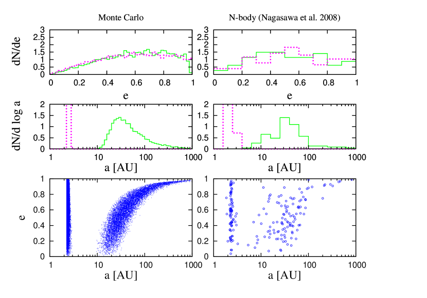
Figure 2: The eccentricity and semimajor axis distributions of surviving planets in the case of three Jupiter-mass planets with $a_{1}=5$AU, $a_{2}=7.25$AU, $a_{3}=9$AU and $e=0$ initially. The dotted and solid lines represent the distributions of inner and outer planets in the top and middle panels. The left panels show the results of $10^{4}$ models generated with our analytic plus Monte Carlo prescription and the right ones are the results of 75 models obtained from Nagasawa et al. (2008)’s N-body simulations.

The comparison of our prescribed method and N-body simulations is shown in Figure 2 where we illustrate the eccentricity and semimajor axis distributions of the surviving planets for a test case with three Jupiter-mass planets ($m_{1}=m_{2}=m_{3}=M_{\rm J}$). We adopt a set of initial conditions with $a_{1}=5$AU, $a_{2}=7.25$AU, $a_{3}=9$AU and $e=0$, in accordance with some existing N-body simulations by Marzari & Weidenschilling (2002) and Nagasawa et al. (2008) (their set N without tidal damping).

The left panels show the results of $10^{4}$ models generated with our analytic plus Monte Carlo prescription and the right panels illustrate the results of 75 models of Nagasawa et al. (2008)’s N-body simulations. The initial orbital phase distributions of planets are modified in each of the N-body simulations. In the analytic plus Monte Carlo simulations, the seed for random number $({\cal R})$ generation to determine eccentricity is changed in each simulation.

The N-body simulations are carried out in 3D, i.e., the orbital inclinations of each planet are also calculated. In our analytic plus Monte Carlo simulations, although the planets’ inclinations are not explicitly computed, their distributions can be evaluated by $i$ (in radian) $\sim e/2$ (Nagasawa et al., 2008).

In this equal-mass example, the top panel of Figure 2 shows that the analytic plus Monte Carlo prescription produces a broad differential eccentricity distribution which is similar for the inner and outer planets. We prescribed (in step B5) a Rayleigh’s distribution through $({\cal R}_{j})$ which has the form $f(e)de=2e\exp(-e^{2})de$ (see Eq. 11). The peak of this distribution function occurs at $1/\sqrt{2}\simeq 0.71$.

The middle panel of Figure 2 shows a bimodal semimajor axis distribution because inwardly scattered planets are generally well separated from outwardly scattered planets. The middle panel of Figure 2 shows a correlation between semimajor axis ($a$) and eccentricity ($e$) of the outwardly scattered planets. This correlation arises because we assume (in step B7) that these planets are scattered from the region near the initial locations and their periastron radii are close to their original semimajor axes despite some outward diffusion before the scattering (see Appendix A2). These results are all consistent with the results obtained by the previous N-body simulations.

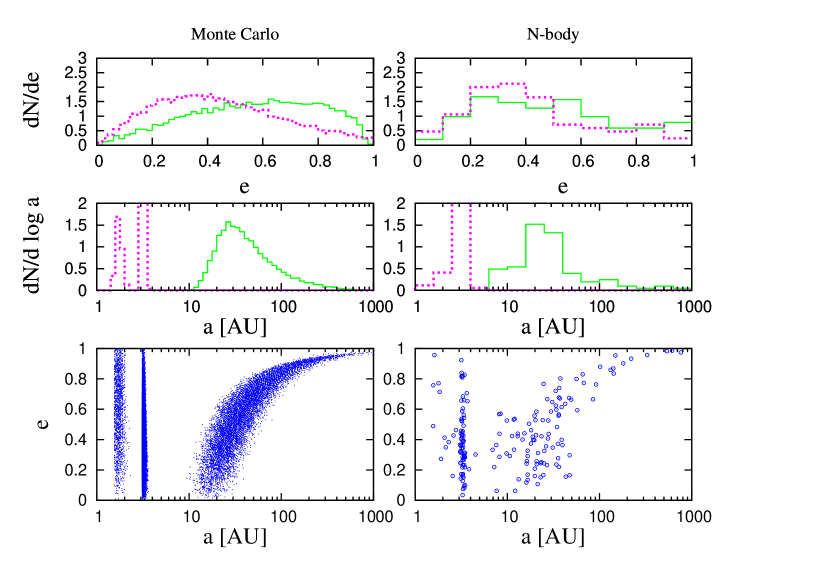
Figure 3: The eccentricity and semimajor axis distributions of the retained planets in the case of $m_{1}=2M_{\rm J},m_{2}=m_{3}=M_{\rm J}$. All other initial conditions are the same as those in Fig. 2.

Marzari & Weidenschilling (2002) also carried out simulations with $m_{1}=2M_{\rm J}$ and $m_{2}=m_{3}=M_{\rm J}$. They found that in 54 runs of 64 runs (corresponds to $\sim 84\%$ probability), the more massive planet (with $m_{1}=2M_{\rm J}$) is scattered inward and the inner retained planets have a broad eccentricity distribution peaked around $e\sim 0.3$. Here, we carry out a similar simulation with the analytic plus Monte Carlo prescription to generate $10^{4}$ models. These results show that the massive planet is scattered inward in 8382 models with a peak eccentricity $1/2\sqrt{2}\simeq 0.36$ (in accordance with eq. (11)).

For comparison purpose, we also simulated 100 N-body models. For the massive planets’ inward scattering probability and their average peak eccentricities, the results obtained with the analytic-plus Monte Carlo prescription are almost consistent with those generated with the N-body simulation, which provides support for the validity of the mass-weighted probability function we have assumed. The middle panel in Fig. 3 show two sharp peaks in the semimajor axis distribution for the inwardly scattered planets. These peaks are also found in the N-body simulations. They are generated from the requirement for energy conservation such that

$$\frac{m_{\rm in}}{a_{\rm in}}\sim\frac{2M_{\rm J}}{5{\rm AU}}+\frac{M_{\rm J}}{7.25{\rm AU}}+\frac{M_{\rm J}}{9{\rm AU}}.$$ (14)

If the inner planet has a mass $m_{\rm in}=M_{\rm J}$ $a_{\rm in}\simeq 1.54$AU whereas $a_{\rm in}\simeq 3.08$AU if $m_{\rm in}=2M_{\rm J}$.

2.4 General case

In the population synthesis simulations, multiple giant planets and rocky/icy planetary embryos co-exist. Here we describe a summary of the prescriptions for dynamical interactions in the general case.

During the early stages of their dynamical evolution, newly formed planets are embedded in and interact with their natal disks. In the presence of the disk gas, we only consider scattering between two planets when their orbital separation $\Delta a$ becomes less than the critical value $\Delta a_{\rm c}\simeq 2\sqrt{3}r_{\rm H}$ with the prescription given in §2.2.

We calculate the planets’ eccentricity damping timescale ($\tau_{\rm damp}$), due to their gravitational interaction with the residual disk, and the orbit-crossing timescale ($\tau_{\rm cross}$) for all pairs of existing planets in gas-free environment. As the disk gas is depleted, $\tau_{\rm damp}$ eventually becomes larger than $\tau_{\rm cross}$ and the planets’ eccentricity grows due to secular excitation (Iwasaki et al., 2002). It then becomes possible for planets with initial separation greater than $\Delta a_{\rm c}\simeq 2\sqrt{3}r_{\rm H}$ to cross each other’s orbits.

Orbital crossings and close encounters among gas giants strongly affect the asymptotic global structure of planetary systems. The gas giants’ eccentricities are highly excited during their orbital crossings. The order of their semimajor axis is occasionally swapped. Their secular resonances may sweep across the entire systems multiple times. Most of the residual small planets are either ejected or collide with their host stars (Matsumura et al., 2013).

For the evaluation on the outcome of planetary scattering after the severe disk-gas depletion, we apply the following prescription. The details are presented in Appendix A3. Note that the order of the prescription presented in this section is different from those in Appendix A3, for the purpose of easier understanding.

C1)

We identify the ”giant planets” from a list of all the planets in the system with the criteria that they have (i) a mass $m>30M_{\oplus}$ and (ii) $e_{\rm esc}>1$ (Eq. 51).

C2-a)

We apply the procedures for orbital crossings among the small planets (as outlined in Paper VI) if there is only one (or less) giant planet.

C2-b)

In systems with two (and only two) widely separated (with $\Delta a>\Delta a_{c}$) giant planets, they retain their initial kinematic properties (because they do not significantly perturb each other). Their dynamical influence on the less-massive planets is computed independently, following the procedures in step C2.

C2-c)

In systems with two (and only two) closely separated (with $\Delta a<\Delta a_{c}$) giant planets, the outcome of their dynamical interaction is computed following steps A2-A3 in §2.2. We also remove all the small planets under the assumption that they are ejected by the gas giants’ sweeping secular resonances.

C2-d)

In systems with 3 or more giant planets around the same host stars, we first evaluate $\tau_{\rm cross}$ for all pairs. For this case,

C3-a)

if $\tau_{\rm cross}$ for all giant planet pairs is longer than the system time ($\tau_{\rm sys}$), we would neglect any interaction between them and compute their influence on the low-mass planets following step C2-a.

C3-b)

If $\tau_{\rm cross}$ for one or more pairs of giant planets is less than $\tau_{\rm sys}$ but there are no triples (overlapping pairs) with $\tau_{\rm cross}<\tau_{\rm sys}$, we would determine the outcome of interaction between the giant planets following step C2-b or C2-c.

C3-c)

Any groups of three giant planets around the same host stars would be labelled as interacting triples if $\tau_{\rm cross}<\tau_{\rm sys}$ for at least two planet pairs. In this case, we follow steps B2-B8 for the triple giants interaction case (see §2.3). All the small planets would be removed under the assumption that they are ejected by the triple giants’ sweeping secular resonances.

C4)

After the kinematic properties of interacting triple systems are modified to a set of new configuration in the previous step, we re-calculate the $\tau_{\rm cross}$ for each pairs of giant planets. Steps C2-C3 are repeated until either 1) there are only two giant planets remaining around the host stars or 2) when $\tau_{\rm sys}+\tau_{\rm cross}>10^{9}$ yrs.

C2-e)

For systems with more than 3 giant planets, we follow the same procedure as C3-a and C4 and eject all the small planets. But, we let only one giant planet be scattered inward and all other giant planets are assumed to be scattered outward.

3 Prescriptions of other physical processes in the population synthesis models

We follow Paper VI for prescriptions of a) planetesimals’ growth through cohesive collisions, b) the evolution of planetesimal surface density, c) embryos’ type I migration, and their stoppage at the disk inner edge. For the gas giants, d) the onset, rate, and termination (through gap opening or and global depletion) of efficient gas accretion, and e) their type II migration, we follow prescriptions in Paper IV, except for a slight modification on gas accretion termination due to global depletion. Here we present a brief summary.

3.1 Disk models

We adopt the minimum mass solar nebula (MMSN) model (Hayashi, 1981) as a fiducial set of initial conditions for planetesimal surface density ($\Sigma_{d}$) and introduce a multiplicative factor ($f_{d}$). For gas surface density $\Sigma_{g}$, although we adopt the $r$-dependence of steady accretion disk with constant $\alpha$ viscosity ($\Sigma_{g}\propto r^{-1}$), rather than that of the original MMSN model ($\Sigma_{g}\propto r^{-1.5}$), we scale $\Sigma_{g}$ by that of the MMSN at 10AU with a scaling factor ($f_{g}$). Following Paper IV, we set

$$\left\{\begin{array}[]{ll}\Sigma_{d}&=\Sigma_{d,10}\eta_{\rm ice}f_{d}(r/{\rm 10AU})^{-1.5},\\ \Sigma_{g}&=\Sigma_{g,10}f_{g}(r/{\rm 10AU})^{-1},\end{array}\right.$$ (15)

where normalization factors $\Sigma_{d,10}=0.32{\rm g/cm}^{2}$ and $\Sigma_{g,10}=75{\rm g/cm}^{2}$ correspond to 1.4 times of $\Sigma_{g}$ and $\Sigma_{d}$ at 10AU of the MMSN model, and the step function $\eta_{\rm ice}=1$ inside the ice line at $a_{\rm ice}$ (eq. [17]) and 4.2 for $r>a_{\rm ice}$ [the latter can be slightly smaller ($\sim 2-3$) (Pollack et al., 1994)]. We specify an inner disk boundary where $\Sigma_{g}$ vanishes and planetesimals’ type I migration is arrested (see §3.5).

Neglecting the detailed energy balance in the disk (Chiang & Goldreich, 1997; Garaud & Lin, 2007), we adopt the equilibrium temperature distribution of optically thin disks prescribed by Hayashi (1981) such that

$$T=280\left(\frac{r}{1{\rm AU}}\right)^{-1/2}\left(\frac{L_{*}}{L_{\odot}}\right)^{1/4}{\rm K},$$ (16)

where $L_{*}$ and $L_{\odot}$ are stellar and solar luminosity. We set the ice line to be that determined by an equilibrium temperature (eq. [16]) in optically thin disk regions,

$$a_{\rm ice}=2.7(L_{\ast}/L_{\odot})^{1/2}{\rm AU}.$$ (17)

The effects of evolution of the disk temperature and associated migration of the ice line adopting more realistic thermal disk structure (Garaud & Lin, 2007; Oka et al., 2011; Min et al., 2011) will be studied in a subsequent paper.

Dependence of disk metallicity is attributed to distribution of $f_{d,0}=f_{g,0}10^{{\rm[Fe/H]}_{d}}$, where $f_{d,0}$ and $f_{g,0}$ are initial values of $f_{d}$ and $f_{g}$, respectively. Due to viscous diffusion and photoevaporation, $f_{g}$ decreases with time. For simplicity, we adopt

$$f_{g}=f_{g,0}\exp(-t/\tau_{\rm dep}),$$ (18)

where $\tau_{\rm dep}$ is disk lifetime (for detailed discussion, see Paper IV). The constant $\alpha$ self-similar solution obtained by Lynden-Bell & Pringle (1974) is expressed by $\Sigma_{g}\propto r^{-1}$ with an asymptotic exponential cut-off at radius $r_{\rm m}$ of the maximum viscous couple. In the region at $r<r_{\rm m}$, $\Sigma_{g}$ decreases uniformly independent of $r$ as the exponential decay does, although the time dependence is different. In the self-similar solution, $\Sigma_{g}$ at $r<r_{\rm m}$ decays as $\Sigma_{g}\propto(t/\tau_{\rm dep}+1)^{-3/2}$. In the exponential decay model that we adopt, $\Sigma_{g}$ decays more rapidly as $t/\tau_{\rm dep}$ becomes larger at $t>\tau_{\rm dep}$. If the effect of photoevaporation is taken into account, $\Sigma_{g}$ decays rapidly after it is significantly depleted, so that the exponential decay partially mimics the effect of photoevaporation. However, the final planet distributions hardly depend on whether $\Sigma_{g}\propto(t/\tau_{\rm dep}+1)^{-3/2}$ or $\Sigma_{g}\propto\exp(-t/\tau_{\rm dep})$. In this paper, we adopt $\alpha=10^{-3}$. The parameter values of $f_{g,0}$, $\tau_{\rm dep}$, and [Fe/H] are specified for each run.

3.2 From Oligarchic Growth to Isolation

On the basis of oligarchic growth model (Kokubo & Ida, 1998, 2002), growth rate of embryos/cores at any location $a$ and time $t$ in the presence of disk gas, is described by $dM_{\rm c}/dt=M_{\rm c}/\tau_{\rm c,acc}$ where, after correcting some typos in Paper IV,

$$\tau_{\rm c,acc}=3.5\times 10^{5}\eta_{\rm ice}^{-1}f_{d}^{-1}f_{\rm g}^{-2/5}\left(\frac{a}{1{\rm AU}}\right)^{5/2}\left(\frac{M_{\rm c}}{M_{\oplus}}\right)^{1/3}\left(\frac{M_{\ast}}{M_{\odot}}\right)^{-1/6}{\rm yrs},$$ (19)

where $M_{\rm c}$ is the mass of the embryo (core), and we set the mass of the typical field planetesimals to be $m=10^{20}$g.

If type I migration is not effective, embryos would formed through oligarchic growth and attain a local isolation mass, $M_{\rm c,iso}=2\pi r\Sigma_{d}\Delta a_{\rm c}$ where the full width of feeding zone of an embryo with a mass $M_{\rm c}$ is given by (Kokubo & Ida, 1998, 2002)

$$\Delta a_{\rm c}\simeq 10r_{\rm H}=10\left(\frac{2M_{\rm c}}{3M_{\ast}}\right)^{1/3}a,$$ (20)

and $r_{\rm H}$ is the Hill radius for two bodies with comparable masses. From equations (15) and (20) we find

$$M_{\rm c,iso}\simeq 0.16\eta_{\rm ice}^{3/2}f_{d}^{3/2}\left(\frac{a}{1\mbox{AU}}\right)^{3/4}\left(\frac{M_{\ast}}{M_{\odot}}\right)^{-1/2}M_{\oplus}.$$ (21)

However, type I migration may induce embryos to migrate before they acquire all the residual planetesimals within their feeding zone and acquire their isolation mass. Type I migration may also be stalled near some trapping radius. At these locations, the congregation of planetesimals may increase the magnitude of $\Sigma_{d}$ and enlarge the magnitude of $M_{\rm c,iso}$.

We compute the evolution of $\Sigma_{d}$ distribution due to accretion by all the emerging embryos in a self-consistent manner. The growth and migration of many planets are integrated simultaneously with the evolution of the $\Sigma_{d}$-distribution. We set up linear grids for $f_{d}$ across the disk with typical width of $\sim 10^{-3}$AU. We introduce a population of seed embryos, all with an initial mass $10^{20}$g (i.e., that of the residual planetesimals) and compute their mass accretion rate. In the inner disk region, we set their initial separation of the full feeding-zone width ($\Delta a_{\rm c}=10r_{\rm H}$) of embryos with local asymptotic isolation mass $M_{\rm c,iso}$.

The planetesimals’ growth time scale increases rapidly with their distance from the central stars and embryos in the outer disk region of the disk are unlikely to attain a local isolation masses within the life span of their host stars. There, we place seed embryos which are separated by feeding zone width of embryos with masses evaluated (using Eq 19) for the local $\Sigma_{d}$ after $t\sim 1$ Gyr. We follow the growth of the seed embryos due to planetesimal accretion in accordance with Eqs. (19) and (20). The planetesimals’ mass accreted by the embryos is uniformly subtracted within the embryos’ current feeding zone. We follow the evolution of $\Sigma_{d}$ throughout the disk and use its values to evaluate embryos’ local accretion rates. We also use $\Sigma_{d}(r,t)$ to estimate the strength of planetesimals’ dynamical friction on the embryos.

During the early phase of evolution, embryos are embedded in their natal disks. Despite their mutual gravitational perturbation, the embryos preserve their circular orbits due to the gravitational drag from disk gas(Artymowicz, 1993; Ward, 1993) and dynamical friction from the residual planetesimals(e.g., Stewart & Ida, 2000). However, after the disk gas is severely depleted, the efficiency of eccentricity damping mechanism is reduced. The embryos’ eccentricity grow until they cross each others’ orbits. We use the prescription in Paper VI and Appendix A3 to compute the occurrence and consequence of giant impacts between embryos.

3.3 Type I migration

Type I migration of an embryo is caused by the sum of tidal torque from the disk regions both interior and exterior to the embryos. The rate and direction of embryos’ migration are determined by the differential Lindblad and corotation torques. While a conventional formula of type I migration assuming locally isothermal disks (e.g., Tanaka et al., 2002) shows that the migration is always inward, recent developments of type I migration of isolated embryos in non-isothermal disks (e.g., Paardekooper et al., 2011) show the magnitude and sign of the tidal torque, especially that due to corotation resonances is a sensitive function of the surface density and temperature distribution of the disk gas.

Since the properties of migration depend on detailed thermal/dynamical structure of disks and ”saturation” degree of the corotation torque (e.g., Kretke & Lin, 2012), substantial discussions are required for the effects of type I migration in non-isothermal disks. The pace of individual embryos’ type I migration in dense multiple planet systems remains uncertain because mutual perturbation between nearest neighbors may modify their Lindblad and especially corotation torque. On the other hand, as shown below, the eccentricity distributions that we are primarily interested in here are not sensitive to a change in the formula of type I migration. Thereby, in order to highlight the validity of our treatment of dynamical interaction between multiple planets in this paper, we postpone the detailed discussions on the non-isothermal type I migration to a subsequent paper. While we also show a result with a non-isothermal formula, in most of the results we present here, we use a conventional formula of type I migration in isothermal disks derived by Tanaka et al. (2002) with a scaling factor $C_{1}$:

$$\begin{array}[]{ll}\tau_{\rm mig1}&{\displaystyle=\frac{a}{\dot{a}}=\frac{1}{C_{1}}\frac{1}{3.81}\left(\frac{c_{s}}{a\Omega_{\rm K}}\right)^{2}\frac{M_{*}}{M_{p}}\frac{M_{*}}{a^{2}\Sigma_{g}}\Omega_{\rm K}^{-1}}\\ &{\displaystyle\simeq 1.5\times 10^{5}\times\frac{1}{C_{1}f_{g}}\left(\frac{M_{\rm c}}{M_{\oplus}}\right)^{-1}\left(\frac{a}{1{\rm AU}}\right)\left(\frac{M_{*}}{M_{\odot}}\right)^{3/2}\;{\rm yrs}.}\end{array}$$ (22)

The expression of Tanaka et al. (2002) corresponds to $C_{1}=1$, and for slower migration, $C_{1}<1$. We study a dependence of the eccentricity distribution by changing a value of $C_{1}$, rather than using variations of non-isothermal formula.

We assume type I migration ceases inside the inner boundary of the disk, because $f_{g}$ is locally zero there. For computational convenience, we set the disk inner boundary to be the edge of the magnetospheric cavity at $\sim 0.04$ AU.

3.4 Formation of gas giant planets

Prescriptions for formation of gas giant planets are the same as those used in Paper IV, except for slight modification for reduction and termination of gas infall. Embryos are surrounded by gaseous envelopes when their surface escape velocity becomes larger than the sound speed of the surrounding disk gas. When their mass grow (through planetesimal bombardment) above a critical mass

$$M_{\rm c,hydro}\simeq 10\left(\frac{\dot{M}_{\rm c}}{10^{-6}M_{\oplus}/{\rm yr}}\right)^{0.25}M_{\oplus},$$ (23)

both the radiative and convective transport of heat become sufficiently efficient to allow their envelope to contract dynamically(Ikoma et al., 2000).

In the above equation, we neglected the dependence on the opacity in the envelope (see Paper I and Hori & Ikoma (2010)). In regions where the cores have already acquired isolation mass, their planetesimal-accretion rate $\dot{M}_{\rm c}$ would be much diminished (Ikoma et al., 2000; Zhou et al., 2007) and $M_{\rm c,hydro}$ can be comparable to an Earth mass $M_{\oplus}$. But, gas accretion also releases energy and its rate is still regulated by the efficiency of radiative transfer in the envelope such that

$$\frac{dM_{p}}{dt}\simeq\frac{M_{p}}{\tau_{\rm KH}},$$ (24)

where $M_{\rm p}$ is the planet mass including gas envelope.

In Paper I, we approximated the Kelvin-Helmholtz contraction timescale $\tau_{\rm KH}$ of the envelope with

$$\tau_{\rm KH}\simeq\tau_{\rm KH1}\left(\frac{M_{p}}{M_{\oplus}}\right)^{-k2},$$ (25)

where $\tau_{\rm KH1}$ is the contraction timescale for $M_{p}=M_{\oplus}$. Since there are uncertainties associated with dust sedimentation and opacity in the envelope(Pollack et al., 1996; Helled et al., 2008; Hori & Ikoma, 2011), we adopt a range of values $\tau_{\rm KH1}=10^{8}-10^{10}$ years and $k2=3$–4. Here we fix $k2=3$ and change $\tau_{\rm KH1}$ (In a nominal case, we use $\tau_{\rm KH1}=10^{9}$ years).

Equation (24) shows that $dM_{\rm p}/dt$ rapidly increases as $M_{p}$ grows. But, it is limited by the global gas accretion rate throughout the disk and by the process of gap formation near the protoplanets’ orbits. The disk accretion rate is

$$\dot{M}_{\rm disk}\simeq 3\pi\Sigma_{g}\nu\simeq 3\times 10^{-9}f_{g}\left(\frac{\alpha}{10^{-3}}\right)\;[M_{\odot}/{\rm yr}].$$ (26)

During the advanced stage of disk evolution, we assume both $\dot{M}_{\rm disk}$ and $\Sigma_{g}$ evolves $\propto\exp(-t/\tau_{\rm dep})$ where $\tau_{\rm dep}$ is the gas depletion time scale. The rate of accretion onto the cores cannot exceed ${\dot{M}_{\rm disk}}$.

An (at least partial) gap is formed when the planets’ tidal torque exceeds the disk’s intrinsic viscous stress (Lin & Papaloizou, 1985). This viscous condition for gap formation is satisfied for planets with

$$M_{p}>M_{\rm g,vis}\simeq 30\left(\frac{\alpha}{10^{-3}}\right)\left(\frac{a}{1{\rm AU}}\right)^{1/2}\left(\frac{L_{\ast}}{L_{\odot}}\right)^{1/4}M_{\oplus}.$$ (27)

Then, type I migration is switched to type II migration. Fluid dynamical simulations (e.g., D’Angelo et al., 2003; D’Angelo & Lubow, 2008) show that some faction of gas still flows into the gap. According to this, we allow a protoplanet to continue accreting the residual gas which flows past it, as shown below. These fluid dynamical simulations, however, also show that the accretion rate rapidly decreases with $M_{p}$ after $M_{p}$ exceeds a Jupiter mass. According to this result and the analysis by Dobbs-Dixon et al. (2007), we completely terminate gas accretion, when the planet’s Hill radius ($r_{\rm H}$) becomes larger than 2 times of disk scale height ($H$), which corresponds to (extended) thermal condition (Lin & Papaloizou, 1985), that is,

$$M_{p}>M_{\rm g,th}\simeq 0.95\times 10^{3}\left(\frac{a}{1{\rm AU}}\right)^{3/4}\left(\frac{L_{\ast}}{L_{\odot}}\right)^{3/8}\left(\frac{M_{\ast}}{M_{\odot}}\right)^{-1/2}M_{\oplus}.$$ (28)

In general, our prescriptions for gas accretion rates onto the cores are

$$\frac{dM_{p}}{dt}=f_{\rm gap}\dot{M}_{p,{\rm nogap}},$$ (29)

where $\dot{M}_{p,{\rm nogap}}$ is that in the absence of any feedback on the disk structure, i.e., that without the effect of gap opening,

$$\dot{M}_{p,{\rm nogap}}=\min\left(\frac{M_{\rm p}}{\tau_{\rm KH}},\dot{M}_{\rm disk}\right),$$ (30)

and $f_{\rm gap}$ is a reduction factor due to gap opening,

$$f_{\rm gap}=\left\{\begin{array}[]{ll}1&[{\rm for}\;M_{p}<M_{\rm g,vis}]\\ \displaystyle{\frac{\log M_{p}-\log M_{\rm g,vis}}{\log M_{\rm g,th}-\log M_{\rm g,vis}}}&[{\rm for}\;M_{\rm g,vis}<M_{p}<M_{\rm g,th}]\\ 0&[{\rm for}\;M_{p}>M_{\rm g,th}].\end{array}\right.$$ (31)

The formula for $M_{\rm g,vis}<M_{p}<M_{\rm g,th}$ is constructed to avoid any abrupt truncation. Some gas may leak through the gap. But, for planets with $M_{p}>M_{\rm g,th}$(D’Angelo et al., 2003), the diffuse gas flows along horseshoe streamlines without being accreted by the planet (Dobbs-Dixon et al., 2007). Further discussion on this issue will be discussed in a future paper.

In Papers I-III, we incorporated the effect of the global depletion by setting a limiting value for the planet’s mass to be $M_{p}<M_{\rm g,noiso}\sim\pi a^{2}\Sigma_{g}$. This prescription was modified in Paper IV, in which we constrained $M_{p}<\int_{0}^{2a}2\pi a\Sigma_{g}da$. These previous prescriptions do not take into account of the viscous diffusion of gas from other disk regions. In order to consider the possibility that gas accretion may also occur in the inner disk regions where the local gas content is limited, we evaluate in this paper both $\dot{M}_{p,{\rm nogap}}$ and $\dot{M}_{\rm disk}$ using the instantaneous values of $\Sigma_{g}$ $(\propto\exp(-t/\tau_{\rm dep}))$. The quenching of gas accretion due to the disk’s global depletion is taken into account without any additional specification. This modification enables us to compute the gas accretion rate onto cores with relatively small semimajor axis.

3.5 Type II migration

During the gap formation, embedded gas giants adjust their positions in the gap to establish a quasi equilibrium between the torque applied on them from the regions of the disk both interior and exterior to their orbits. Subsequently, as the disk gas undergoes viscous diffusion, this interaction leads to type II migration.

We assume that planets undergo type II migration after they have accreted a sufficient mass to satisfy the viscous ($M_{\rm g,vis}<M_{p}$) condition for gap formation, as commented in section 3.4.

While $M_{p}$ increases, the disk mass declines due to stellar and planetary accretion and photoevaporation. While the disk mass exceeds $M_{p}$ (during the disk-dominated region), planets’ type II migration is locked with the viscous diffusion of the disk gas. During the advanced stages of the disk evolution when its mass become smaller than $M_{p}$ (during the planet-dominated region), the embedded planets carry a major share of the total angular momentum content. A significant fraction of the total (viscous plus advective) angular momentum flux transported by the disk gas is absorbed by the planet in its orbital evolution (for detailed discussion, see Paper IV).

For the disk-dominated regime, the migration timescale is given by

$$\begin{array}[]{ll}\tau_{\rm mig2,disk}&{\displaystyle=\mid\frac{a}{\dot{a}}\mid=\frac{a}{(3/2)\nu/a}}\\ &{\displaystyle\simeq 0.7\times 10^{5}\left(\frac{\alpha}{10^{-3}}\right)^{-1}\left(\frac{a}{1{\rm AU}}\right)\left(\frac{M_{*}}{M_{\odot}}\right)^{-1/2}}\;{\rm yrs}.\end{array}$$ (32)

For the temperature distribution given by Eq. (16), $\nu\propto r$ and $\tau_{\rm mig2,disk}$ reduces to

$$\tau_{\rm mig2,disk}=\frac{a}{r_{\rm m}}\frac{2r_{\rm m}^{2}}{3\nu(r_{\rm m})}\simeq\frac{a}{r_{\rm m}}\tau_{\rm dep},$$ (33)

where $\tau_{\rm dep}$ is global disk viscous-evolution time scale and $r_{\rm m}$ is the disk radius where the viscous couple attains a maximum value. (The magnitude of $r_{\rm m}$ is approximately the characteristic disk size). In general, $\tau_{\rm mig2,disk}$ is a fraction of the disk lifetime except for the planets which formed near $r_{\rm m}$.

Observationally inferred disk lifetime is 1-10Myrs. If this lifetime is comparable to the disk viscous-evolution time scale, $r_{\rm m}\sim(15-150)\times(\alpha/10^{-3})$AU. In this limit, Eq. (33) would imply that many gas giants form just beyond the snow line migrate to the proximity of their host stars and become hot Jupiters unless they emerged during the advanced (planet-dominated) stage of disk evolution or the type II tidal torque is significantly reduced by the disk flow through the gap or by the mutual interaction between multiple planets and their natal disks.

In Paper IV, we showed that the type II migration time scale in the planet-dominated regime can be evaluated in terms of

$$\begin{array}[]{ll}\tau_{\rm mig2,pl}&{\displaystyle=\frac{1}{C_{2}}\frac{(1/2)M_{p}a^{2}\Omega_{\rm K}(a)}{\dot{M}_{\rm disk}r_{m}^{2}\Omega_{\rm K}(r_{m})}=\frac{1}{2C_{2}}\left(\frac{a}{r_{\rm m}}\right)^{1/2}\frac{M_{p}}{\dot{M}_{\rm disk}}}\\ &{\displaystyle\simeq 5\times 10^{5}f_{g}^{-1}\left(\frac{C_{2}\alpha}{10^{-4}}\right)^{-1}\left(\frac{M_{\rm p}}{M_{\rm J}}\right)\left(\frac{a}{1{\rm AU}}\right)^{1/2}\left(\frac{r_{\rm m}}{10{\rm AU}}\right)^{-1/2}\left(\frac{M_{*}}{M_{\odot}}\right)^{-1/2}}\;{\rm yrs},\end{array}$$ (34)

where $C_{2}$ is an efficiency factor associated with the degree of asymmetry in the torques between the inner and outer disk regions. If the inner disk is severely depleted, $C_{2}=1$. But, in evolving disks with comparable surface density on either sides of multiple planets, the degree of torque asymmetry has large uncertainties in both the disk and planet dominated regimes. Although the reduction factors for the disk and planet-dominated regimes may be independent from each other, we adopt the same reduction factor $C_{2}$ for both regime and treat the factor $C_{2}$ as a model parameter. In the results shown in this paper, we set $C_{2}=0.1$. The kinematic distribution of the planets are weakly affected by the choice of $C_{2}$, as long as $C_{1}\gtrsim 0.03$. The eccentricity distribution of the emerging gas giant planets is not strongly affected by the magnitude of $C_{2}$.

3.6 Resonant capture

The pace of both type I and II depends on both the disk structure and $M_{p}$. As different-mass planets migrate, the separation between their semimajor axis may either increase or decrease through divergent and convergent migration respectively. Multiple planets may also converge near some special disk locations such as the edge of the magnetospheric cavity near the inner disk boundary. As the migration of first-born planets is stalled at these trapping radii, later-generation planets may continue to arrive.

The planets gradually converging orbits capture each other on their mutual mean-motion resonances provided their migration time scale across the resonances’ width is shorter than the resonances’ libration time scales. After they enter into their mean motion resonances, these planets have a tendency to migrate together while maintaining the ratio of their semimajor axes (McNeil et al., 2005; Ogihara & Ida, 2009). In their simulations, Ogihara & Ida (2009) and Ogihara et al. (2010) found that outside the disk inner boundary at $\sim 0.1-0.3$AU, it is possible for a few dozen rocky planetary embryos to be trapped in adjacent embryos’ mean-motion resonances. During and after the depletion of the disk gas, their orbits become unstable, they undergo orbit crossing and cohesive collisions to merge into a few super-Earths.

In Paper VI, we implemented a prescription for resonant capture between rocky/icy planets into our sequential planet formation model. With this prescription, we constructed population synthesis models for multiple super-Earth systems. These simulations showed a rich population of embryos accumulate near the inner disk boundary. Although differential migration leads to embryos’ orbital convergence, stochastic secular perturbation between multiple embryos induces orbital diffusion. Instead of locking into the most widely separated 2:1 mean motion resonances, the nearest neighbors are packed into low-order main-motion resonance with semimajor axis separations comparable to several $r_{\rm H}$. The Hill radius $r_{\rm H}$ is defined to be $r_{\rm H}=((m_{i}+m_{j})/3M_{\ast})^{1/3}a$ where $m_{i}$ and $m_{j}$ are the masses of the closest pairs, $M_{*}$ is the host star’s mass, and $a=\sqrt{a_{i}a_{j}}$ is mean semimajor axis of the pair.

For computational simplicity, we adopted in Paper VI, a prescription that, as a consequence of converging migration, the closest embedded embryo pairs enter into and are locked in mean motion resonances with a separation of $5r_{\rm H}$ between their semimajor axes. After capture each other, the resonant embryos migrate in steps while maintaining their semimajor axis ratios and sharing angular momentum loss associated with the gravitational interactions between the disk and individual embryos.

In the present paper, we consider the possibility that the converging differential migration may proceed so rapidly that the neighboring embryos may not have time to capture each other into mean motion resonances. We evaluate the condition for a dynamical equilibrium in which convergence time scale (due to differential migration) matches with the mean motion libration time scale (see Paper VI). If this equilibrium is established with an orbital separation which is less than $\Delta a_{\rm c}\simeq 2\sqrt{3}r_{\rm H}$, we assume the converging embryos will collide and coalesce (see §2.2).

We further extend the resonant capture condition for planet pairs including both super-Earths and gas giants. Based on the rate of orbital decay due to gas drag, Shiraishi & Ida (2008) derived a criterion for non-resonant planetesimals to enter the feeding zone of a growing gas giant. Here we adopt their criterion for the embryos, the migration of which is determined by their tidal interaction with the disk gas. We replace the migration rate due to gas drag with differential speed between type II migration of a giant and type I migration of rocky/icy embryos.

In the case that a planet (an embryo or another giant) enters a feeding zone of a gas giant, we apply the prescription in §2.1 to determine the outcome of their encounters. Although the treatment in §2.1 is constructed for scattering between two gas giants, the same prescriptions are also applicable for the case where an embryo is scattered by a giant. In this limit, the perturbations from the giant is so strong and dominant that these events tend to result in the ejection of the embryos or in widely separated orbits rather than cohesive collisions.

In Paper VI, we assumed that the disk inner edge is a rigid wall for type I migration of embryos. This assumption is based on a strong ”eccentricity trapping” effect(Ogihara et al., 2010). The torque exerted onto the innermost embryo in an eccentric orbit is so strong that it can halt the type I migration and offset the angular momentum loss of several outer embryos. The magnitude of torque associated with embryos-planet interaction depends on the planet’s mass. The condition for a single planet (with a mass $m_{1}$) to frustrate the inner migration of other embryos (with masses $m_{j}$ $(j\geq 2)$) at the inner boundary (Ogihara et al., 2010) is

$$\sum_{j=1}m_{j}^{2}<\frac{5}{C_{1}}m_{1}^{2}.$$ (35)

Leakage of innermost embryo across the disk inner boundary would be imposed if the above condition is not satisfied. We also allow the leakage of embryos across the disk inner boundary if they lie in the path of an inwardly migrating gas giant planet.

4 Simulated individual systems

Before we enter into an comprehensive discussion on the statistical properties and population synthesis of multiple-planet systems, we first highlight the dynamical interaction among several bodies around common host stars with a few sample simulations of individual systems. Such studies have not been possible with the ”one-planet-per-disk-model” prescription in which planet-planet interactions are neglected (e.g., Papers I-V and the models of Mordasini et al. (2009a, b)).

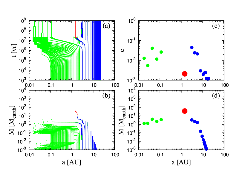
Figure 4: Growth and migration of planets in a system with $C_{1}=0.1$ and $f_{d,0}=2.0$. In the color version, the green, blue and red lines represent planets with their main component is rock, ice and gas, respectively.

For illustration purpose, we choose for Model 1, $C_{1}=0.1$, $f_{g,0}=f_{d,0}=2.0$ ([Fe/H]$=0$), $\tau_{\rm KH1}=10^{9}$ years, $\tau_{\rm dep}=3\times 10^{6}$ years around a solar-mass star ($M_{*}=1M_{\odot}$). Figure 4a and b show time and mass evolution of planets for Model 1. The green, blue and red lines represent rocky, icy, and gas giant planets with their main component being rock, ice and gas, respectively. Although rocky and icy planets are formed respectively interior and exterior to the snow line, their migration and dynamical interaction may lead to their spatial diffusion. The main composition of the planets may change through gas or planetesimal accretion or embryo-embryo collisions (giant impacts).

The results in Panel b show that at 0.1–1AU small embryos grow in situ until their masses reach $\sim 0.1M_{\oplus}$ –$1M_{\oplus}$ and then undergo type I migration to accumulate near the inner boundary of their natal disks. We can determine the critical embryo mass for transition from local mass growth to efficient type I migration by matching Eqs. (19) and (22) such that

$$M_{\rm c,max}\simeq 1.0\left(\frac{C_{1}}{0.1}\right)^{-3/4}\left(\frac{f_{g}}{2}\right)^{3/10}\left(\frac{\eta_{\rm ice}f_{d}}{f_{g}}\right)^{3/4}\left(\frac{a}{1{\rm AU}}\right)^{-9/8}\left(\frac{M_{\ast}}{M_{\odot}}\right)^{5/4}M_{\oplus}.$$ (36)

A few small ($10^{-3}M_{\oplus}$–$10^{-2}M_{\oplus}$) embryos are also induced to undergo orbital decay. The orbital evolution of these low-mass embryos is induced by the perturbation from the migrating planets.

Many resonant embryos accumulate in the vicinity of the disk inner boundary which is set to be 0.04 AU (Panel a, Figure  4). These planets are preserved in the disk region provided the condition (35) is satisfied. But when the total mass of the trapped planets in the proximity of the inner disk edge exceeds the critical mass given by eq. (35), innermost planets are driven to cross the disk inner edge until the retention condition in Eq . (35) is restored. In this model, more than half of the embryos arrived in the inner disk region eventually cross its inner boundary. We assume that after planets migrate inside the central magnetospheric cavity in the disk, their tidal and magnetic interaction with their host stars provide an effective torque to induce them to undergo further orbital decay. Note that in the weak-field limit, the size of the magnetospheric cavity is much smaller and the disk inner boundary is adjacent to the stellar surface. In this limit the innermost planets are unlikely to survive (Paper VI).

In the intermediate disk region, a migrating core attains $M_{p}\sim 5M_{\oplus}$ just outside the ice line at $a\sim 3$AU. This core starts its runaway gas accretion without any significant type I migration. When it evolves into a gas giant with a surrounding gap, it undergoes type II migration which is much slower than type I migration. The emerging gas giant scatter and eject nearby embryos (they are represented by the lines which are discontinued at $t\sim 2\times 10^{7}$ yrs.)

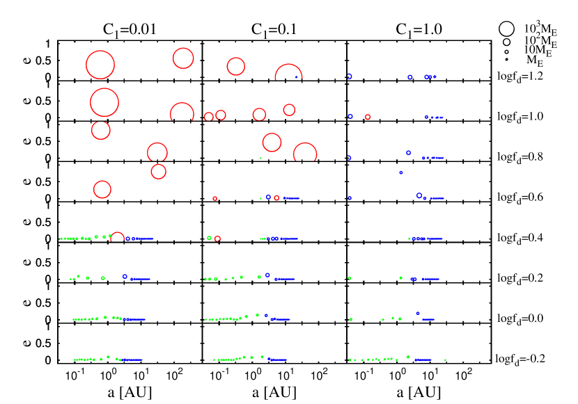
Figure 5: Planetary systems as functions of $C_{1}$ and $f_{d,0}$. The radii of circles are proportional to one cube of planetary masses; legends are shown in upper right of the figure. In the color version, the green, blue and red lines represent planets with their main component is rock, ice and gas, respectively.

In order to explore the dependence of various model parameters, we simulated a series of models with a range of different $C_{1}$ and $f_{d,0}$ values. We use the same values (as Model 1) for [Fe/H]$=0$, $\tau_{\rm dep}=3\times 10^{6}$yrs, and $M_{*}=1M_{\odot}$. The asymptotic distributions of mass, semimajor axis and eccentricity of planets for these models are summarized in Figure 5.

For high values of $C_{1}(=1)$, type I migration is so efficient that gas giants are rarely formed. In runs with $\log f_{d,0}\gtrsim 0$, rocky/icy planets are not retained at $a\lesssim 1$AU except the vicinity of the disk edge at which type I migration is halted.

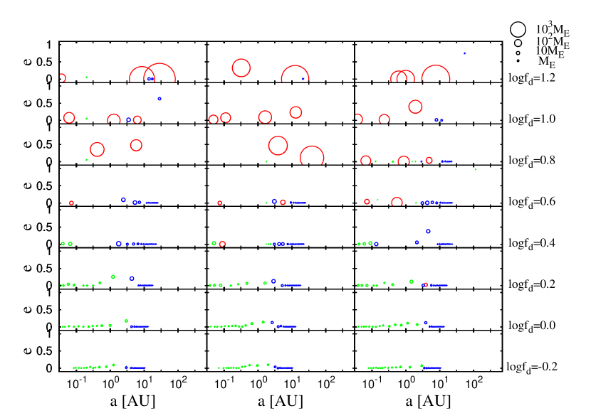
Figure 6: Planetary systems with $C_{1}=0.1$ as functions of $f_{d,0}$. In order to test the dispersion of the simulated results, we choose three random number seeds for the scattering prescription. Models in the middle column are identical to those in the middle column in Figure 5.

For models with $C_{1}=0.1$ and 0.01, the planet distributions are sensitively determined by the total planetesimal mass in the disk, i.e., the value of $\log f_{d,0}$. In our procedures for close scattering (see §2.2) depend on the choice of random number seeds. In order to test the robustness and dispersion of our models, two additional series of models are carried out for $C_{1}=0.1$ with different random number seeds for the scattering prescription (Figure 6).

All these models show similar planetary systems’ dependence on values of $f_{d,0}$. With relatively high values of $f_{d,0}$, the emerging planetary systems consist mostly of gas giants. In these massive disks, the amount of rocky/icy materials is sufficiently large to enable the formation of multiple cores of gas giants. Dynamical instability leads to giant planets to undergo close encounters which excite their eccentricity. Some giant planets may collide and coalesce into massive and eccentric merger products (Lin & Ida, 1997). Other planets attain eccentric orbits including those which are ejected from the system or scattered to endure close encounters with their host stars. During these violent dynamical relaxation, the orbits of rocky/icy planets are strongly perturbed by the giant planets and they are generally not retained.

In contrast, disks with moderate masses (or values of $f_{d,0}$) generally nurture fewer and more widely separated cores. Gas accretion leads to the emergence of either single or widely separated and sparsely populated giant planets. The mass of these planets is determined by the gap formation condition and is generally smaller than that of merger products. The mutual interaction between single gas giant planets and residual embryos or between sparsely populated gas giant planets is generally too weak for them to become dynamical unstable. They then retain relatively low eccentricities.

Comparison of Figures 5 and 6 indicates relatively massive and eccentric gas giant planets are formed out of massive disks whereas disks with modest masses generally produce gas giant planets with lower masses and eccentricities. Through the population synthesis models (next section), we show that this correlation can be used to infer initial formation condition of mature planets long after their natal disks have been depleted.

5 Population Synthesis of Planetary Systems

This set of prescription enable us to incorporate gravitational interactions among planets into our population synthesis models. The main objective of simulating ”multi-planets-in-a-disk” models is to generate mass and eccentricity distributions of the emerging multiple-planet systems. These quantities can be directly compared with observational data.

5.1 Initial conditions

We adopt a range of disk model parameters (see §3.1) and assign each their values with appropriate statistical weights to match the observed distribution of disk properties. We assume that $f_{g,0}$ and $\tau_{\rm dep}$ have log normal distributions in ranges of 0.1–10 and $10^{6}$–$10^{7}$ years, respectively. We use a normal distribution of [Fe/H] in a range of -0.2 to 0.2 which corresponds to that of typical target stars in various on-going radial velocity surveys. Since the target stars of radial velocity surveys are mostly G dwarfs, we use a log normal distribution, in a range of 0.8-$1.25M_{\odot}$, for the host stars’ mass ($M_{*}$).

The initial distributions of seed planetesimals are described in §3.1 and their growth rate and migration time scales are specified in §3.2–3.5. Prescriptions for dynamical interactions among multiple planets are presented in §2.1–2.3 and 3.6.

5.2 Distributions of mass, semimajor axis and eccentricities

The asymptotic $e-a$, $e-M_{p}$, and $M_{p}-a$ distributions of a population of $10^{4}$ multiple-planet systems are shown in Figures 7. Similar to previous figures, the green, blue and red symbols represent rocky, icy and gas giant planets, respectively.

Models with similar parameters have been simulated in Paper IV with the ”one-planet-in-a-disk” prescription. In these previous models, the formation of gas giant planets require a substantial reduction in the pace of their cores’ type I migration (with $C_{1}=0.01-0.03$). This result reflects the requirement for not only the formation but also retention of sufficiently massive cores (§3.6) to efficiently accrete gas. The present prescription bypasses this competition between type I migration and mass growth because it takes into consideration the possibility that multiple embryos may undergo convergent migration, dynamical instability, orbit crossing and close encounters. Coalescence of two or more embryos (with relatively low masses and long type I migration time scales) promote sporadic, substantial mass increases. The merger products can impulsively acquire a critical mass for the onset of gas accretion before they undergo extensive migration.

A direct comparison between Figure 7c and Figure 5 in Paper IV show that, with $C_{1}=0.1$, the new prescription indeed leads to much more prolific production of gas giants. Some of these gas giant planets form during the advanced stages of disk evolution after 90% of the disk gas been depleted. In these low density environment, the eccentricity of embryos may be excited by their perturbation on each other but not effectively damped. Eventually they cross each other’s orbit, merge into sufficiently massive cores to accrete residual disk gas and evolve into gas giant planets.

In contrast to the “one-planet-in-a-disk” models, we can determine, with the new prescription, planets’ velocity dispersion from their mutual interaction in multiple-planet systems. From this kinematic information, we obtain the $e-a$ and $e-M_{p}$ distributions in Figure 7a and c. The ”V” shape centered at a few AU in the $e-a$ distribution is a signature of strong scatterings by the most massive planets in the system which preferentially form near the snow line (at a few AU’s). Less massive planets are either scattered inward, outward, or collide with the gas giant planets. The left/right branch of the “V” corresponds to the loci of planets which have been scattered inward/outward. These inwardly/outwardly scattered planets preserve their apo/peri astrons to be orbital radii of the gas giant planets. Finally, the $e-M_{p}$ distribution shows that eccentricity distribution is uniform or rather increases with $M_{p}$. If we consider only massive planets that are currently observable by radial velocity survey, eccentricity distribution clearly increases with $M_{p}$ as shown below.

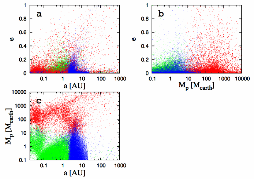
Figure 7: The asymptotic kinematic distributions of a simulated population of planets in multiple-planet systems. For these fiducial models, we adopt $\tau_{KH1}=10^{9}$ yr and $k_{2}=3$ and $C_{1}=0.1$. The eccentricity $e$ versus semimajor axis $a$ distribution is plotted in panel (a). The $e-M_{p}$ distribution is plotted in panel (b). The $M_{p}-a$ distribution is plotted in panel (c). The green, blue and red symbols represent rocky, icy and gas giant planets, respectively.

We compare our simulated population-synthesis models with observational data. In Figures 8, we plot observed (a) $e-M_{p}$, (b) $e-a$, and (c) $M_{p}-a$ distributions in the left, middle, and right columns respectively. The observational data are displayed in the top row. These data include only those planets which were first discovered by radial velocity surveys. We excluded planetary candidates which were first discovered by transit surveys, regardless whether they were confirmed by follow-up radial velocity observations. The main rationale for this selection is that the detection probability by transit surveys is highly biased to short-period planets.

The simulated population of $10^{4}$ multiple-planet systems is plotted in the bottom row. Here $M$ refers to $M_{p}\sin i$ with a distribution of inclination angle $i$ between the line of sight and the planets’ orbital angular momentum axis that assumes random orientations of orbit normals of the planets. Some of these planets have low-mass and large semimajor axis. They are below the present-day detection capability. In order to take into account the limited radial velocity precision and data base line, we selected a subset of data in which the predicted reflective motion of the host stars is larger than 1 m/s and the planets’ orbital period is shorter than 10 years. These “detectable planets” are plotted in the middle row.

Comparison between top and middle panels in Figures 8a and b shows that the theoretical models match well the observed kinematic distributions. Both observations and population synthesis models show that $e$ increases with $M_{p}$ and $a$. In the next subsection, we will show that these correlations are robustly reproduced, almost independent of model parameters.

Most gas giants have semimajor axis $a\gtrsim 0.5$AU. Their eccentricities are not affected by the dissipation of tidal perturbation induced by the host stars on the planets. Detailed comparison of the top and mid row of the middle column indicate that the fraction of high-eccentricity ($e\gtrsim 0.2$) planets in the theoretical model is low ($\sim 10\%$) compared with that ($\sim 50\%$) in observed data. This discrepancy may be observational uncertainties which generally tend introduce over-estimates for planets’ eccentricities. It may also be due the secular perturbations between gas giants which has not yet been incorporated in our prescription. In multiple-planet systems with significant angular momentum deficit, secular interaction can induce large-amplitude angular momentum exchange, eccentricity modulation, and long-term orbital instabilities. A treatment of secular perturbations will be constructed and presented elsewhere.

In this paper, we focus primarily on the planets’ eccentricity distributions. Comparison between top and middle panels in Figure 8c show that our prescription qualitatively reproduces the observed correlations in the $M_{p}-a$ distribution. Whereas the observational data clearly show an over density of gas giants at $a\gtrsim 0.7$AU, their semimajor axis distribution in the simulated population synthesis models is relatively uniform on a log scale. The sensitive dependence of the $M_{p}-a$ distribution on the parameters of population synthesis models will be discussed in detail in the next paper.

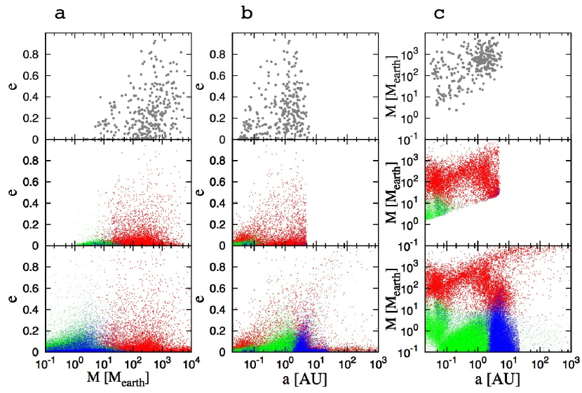
Figure 8: Comparison of theoretical results in a nominal case with observational data: (a) $e-M_{p}$, (b) $e-a$, and (c) $M_{p}-a$ distributions. The top row are the data obtained from radial velocity surveys. The planets that were discovered transit survey and confirmed with follow-up radial velocity observation are excluded. The bottom row are the distributions of planets in $10^{4}$ systems simulated with the updated population-synthesis prescription. Panels in the middle row represent only the simulated observable planets, i.e., those with radial velocities greater than 1 m/s and periods less than 10 years.

5.3 Correlations between eccentricity and mass or semimajor axis

The origin of the correlation of eccentricity and semimajor axis can be traced back through the procedures of our theoretical model. In the observed $e-a$ distribution, $e$ is apparently lower at $a\lesssim 0.1$AU than at $a\sim 1$AU (the top panel in Figure 8b). This correlation has been attributed to the dissipation of stellar tidal perturbation inside the planetary envelope which leads to the orbital circularization of close-in planets. This tidal effects has not yet been implemented in the population synthesis models. Yet, this $e-a$ correlation is also very well established in the simulated results. In Eq. (3), we showed that the maximum eccentricity excited by close scattering between gas giants is $\propto a^{1/2}$, because the two-body surface escape velocity ($v_{{\rm esc},jk}$) is independent of $a$ whereas the Kepler velocity ($v_{\rm K}$) is $\propto a^{-1/2}$. Consequently, in the deep potential near the host stars, it is difficult for close scattering to excite high eccentricities. Based on the above prescription, the maximum $e$ we obtain at $a\sim 0.1$AU is 3 times smaller than that at $a\sim 1$AU in the simulated models (the middle panel in Figure 8b).

Multiple massive giants are preferentially formed in relatively massive disks (see discussions in §4). These dynamically packed systems are more prone to dynamical instabilities, orbit crossing, excitation of high eccentricities and cohesive collisions. A correlation between high eccentricity and planetary mass is naturally expected. In order to verify this scenario, we plot in Figure 9, $e$ and $M_{p}$ of gas giants as a function of $f_{d,0}$ in the fiducial models (in which $\tau_{KH1}=10^{9}$ yr and $C_{1}=0.1$) of Figure 7. This figure clearly shows that, in the range of $f_{d,0}=1-10$, both the mass of gas giants and the fraction of high $e$ planets increase with $f_{d,0}$. Based on this inference, we can infer the distribution of disk masses from the observed $e-M_{p}$ distribution. Raymond et al. (2010) performed N-body simulations of multiiple giant planets with different masses and found a similar correlation between high eccentricity and planetary mass, although their initial conditions are artificial. Note that Figure 9 only includes gas giants at $a<30$AU. As shown in Figures 7a and c, the kinematic distribution of gas giants with $a\gtrsim 30$AU have two (high $e$ and low $e$) components. We discuss this issue in the next subsection.

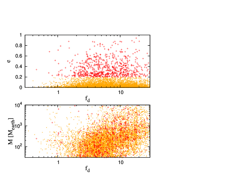
Figure 9: The distributions of $e$ and $M$ of gas giants with $a<30$AU as a function of $f_{d,0}$ in the fiducial models of Figure 7. The thick and thin symbols represent giants with $e>0.2$ and $e<0.2$, respectively (In the color version, red and orange symbols).

The above discussion indicates that the $e-a$ and $e-M_{p}$ correlations are the natural outcome of close scatterings and the formation of gas giants. It also shows that these correlations are insensitive to other physical parameters such as the rate of type I migration rate ($C_{1}$) and the magnitude of the gas accretion timescale ($\tau_{\rm KH1}$). These independences are reflected in Figures 10 and 11 for simulated populations with different values of $C_{1}$ and $\tau_{\rm KH1}$. Although the number of gas giants per host star is lower among populations with relatively high $C_{1}$ and long $\tau_{\rm KH1}$, the trend that $e$ is lower at $a\lesssim 0.1$AU than at $a\sim 1$AU persists.

This trend is less conspicuous in the limit of relatively small $C_{1}$ ($0.03$ in Figures 10) and gas accretion time scale $\tau_{\rm KH1}$ ($10^{8}$ years in Figure 11). In these limits, the prolific formation of gas giants and the high frequency of their close scattering leads to a prominent ”V” feature in the $e-a$ distribution. This feature also affects the distribution of observable planets (displayed in the upper rows of these figures). The lack of any obvious evidences of this “V” feature in the observational data (Figure 8a), places a limit on the efficiency of gas giant formation and constraints on the magnitude of $C_{1}$ and $\tau_{\rm KH1}$. In the fiducial population synthesis model (with $C_{1}=0.1$ and $\tau_{\rm KH1}=10^{9}$ yr), the fraction of solar-type stars that harbor gas giants with $a=0.5-5$AU and $M_{p}>100M_{\oplus}$ (cool jupiters) is 21%. This fraction for both the $C_{1}=0.03$ models (47%) and the $\tau_{\rm KH1}=10^{8}$ years models (42%) are both much higher than that inferred by radial velocity surveys.

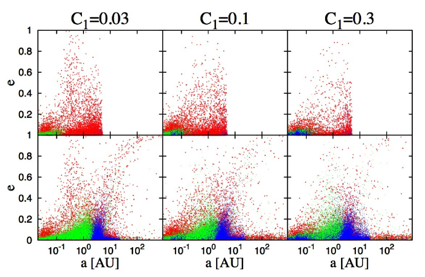
Figure 10: Dependence on $C_{1}$ of the simulated $e-a$ distribution. The lower panels are distributions of $10^{4}$ systems of planets generated with our Monte Carlo simulation. The upper panels contain only the observable (with radial velocities greater than 1 m/s and periods less than 10 years) simulated planets. These observable criteria correspond to the technical limitation of current radial velocity surveys. The left, middle and right panels display results for models with type I migration coefficient $C_{1}=0.03,0.1$ and 0.3, respectively. The symbols are the same as those in Figures 8.

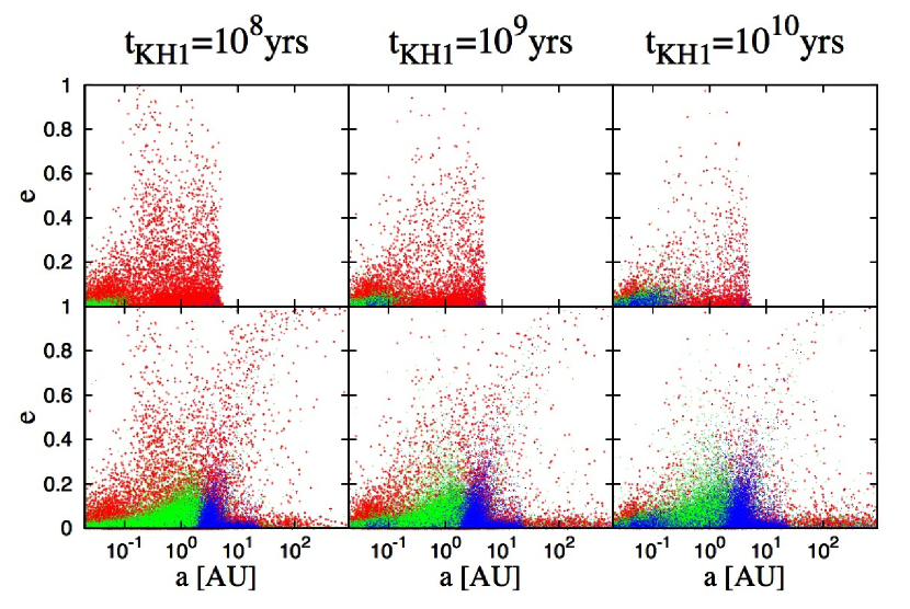
Figure 11: The $e-a$ distribution of simulated models with various values of $\tau_{\rm KH1}$. The left, middle and right panels include results generated with the parameter for envelope contraction timescale (for $M_{p}=M_{\oplus}$) $\tau_{\rm KH1}=10^{8},10^{9}$ and $10^{10}$ years, respectively. The meaning of upper and lower panels are the same as in Figures 10.

Figures 12 and 13 show the dependence of the $e-M_{p}$ distribution on $C_{1}$ and $\tau_{\rm KH1}$, respectively. Although more massive planets, in general, tend to have larger $e$, this trend is less conspicuous for models with $C_{1}=0.3$ and $\tau_{\rm KH1}=10^{10}$ years. In these limiting cases, the formation of gas giants is affected by the rapid migration of the cores and slow gas accretion. These restrictions are more severe for formation of the relatively massive gas giants. Despite these extreme cases, the correlations in $e-a$ and $e-M_{p}$ distributions are well established in the population synthesis models for a wide range of parameters. The general reproduction of the observed correlations suggests that these properties are associated with close scattering among gas giants.

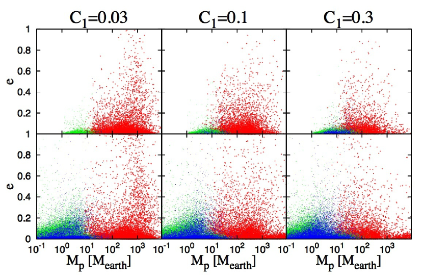
Figure 12: Dependence on $C_{1}$ of the predicted $e-M_{p}$ distribution. The meaning of panels are the same as in Figures 10.

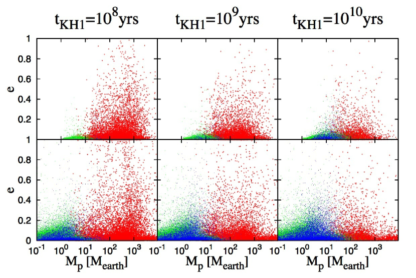
Figure 13: Dependence on $\tau_{\rm KH1}$ of the predicted $e-M_{p}$ distribution. The meaning of panels are the same as in Figures 11.

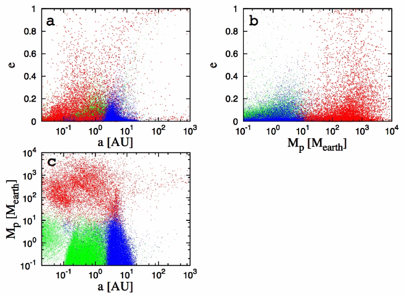
Figure 14: Same as Figure 7 except for use of non-isothermal type I migration formula instead of isothermal one with $C_{1}=0.1$.

In Figures 14a, b and c, we show the $e-a$, $e-M_{p}$ and $M_{p}-a$ distributions with the non-isothermal type I migration formula. Because in inner (optically thick) disk regions, migration is outward for some range of $M_{p}$ (Kretke & Lin, 2012), many gas giants survive even without any reduction in amplitude of the migration velocity. While the $M_{p}-a$ distribution is affected by the different migration formula, the $e-a$ and $e-M_{p}$ distributions are similar to those obtained by the isothermal migration formula and they are within a range of variations of the results with different values of $C_{1}$ and $\tau_{\rm KH1}$ in figures  10, 11, 12 and 13. Therefore, here we do not go into the details of the non-isothermal migration formula and focus on the eccentricity distributions obtained with the isothermal migration formula and a scaling factor $C_{1}$, as discussed in §3.3.

5.4 Formation of distant large gas giants in circular orbits

The population synthesis models also generate a population of massive ($M_{p}\gtrsim 10M_{J}$) gas giants with large semimajor axis ($a\gtrsim 30$AU) (Figure 7c). In principle, these planets can be observationally detected during their infancy with direct imaging searches. In the fiducial models, the fraction of host stars that have these planets is $\sim 3.7\%$ and most of them have low-eccentricity ($e\lesssim 0.1$) orbits (Figure 7a). If these planet were grown to gas giants near the snow line and scattered to these large distances, they would preserve their periastron distance. For example, planets formed interior to 30 AU may be scattered to attain a semimajor axis $ga100$ AU with an $e\gtrsim 0.7$. Although the effect of eccentricity damping is included in our prescription for disk-planet interaction, its efficiency is generally too low to account for the low eccentricity of distant, massive planets generated in these population synthesis models (step 3-a of Appendix A1).

A close inspection of our results yields an alternative path for the formation of distant gas giant planets. In systems which contain multiple gas giants, the rapid gas accretion of first generation gas giants destabilize the orbits of nearby residual embryos. Some embryos are scattered to large distance where the surface densities of both residual planetesimals and gas are relatively low. Because the scattered embryo masses are usually well below the local disk mass, even the relatively low surface density gas damps the eccentricity of the scattered embryos to the level below 0.1 (also see the discussion below).

A reduction in the planetesimal accretion rate at these distance also lowers the critical core mass for the onset of gas accretion (see Eq. 23). In extended protostellar disks, there is adequate supply of gas supply, even during the advanced stages of disk evolution to enable the circularized planets to acquire masses larger than that of Jupiter.

The ratio of planets’ asymptotic mass to that of their host stars is a monotonically increasing function of their natal disks’ aspect ratio which is also an increasing function of $a$ (see Eqs. 27 and 28). The simulated populations confirm that the masses of the long-period gas giants are robustly correlated with $a$ in the fiducial (Figure 7c) and other models. If this trend is confirmed by observation, it provides evidence to support the scenario that long-period, low-eccentricity, massive gas giants are the byproducts of gas accretion onto outwardly scattered cores.

During the course of mass accretion, the planets also acquire angular momentum of the disk gas. Although the scattered embryos have high eccentricity initially, they gain angular momentum through planet-disk tidal interaction. Our prescription for the eccentricity damping may be less efficient than that, due to supersonic relative velocity between the core and disk gas (Ostriker, 1999; Papaloizou & Larwood, 2000; Muto et al., 2010), although it nonetheless may lead to the circularization of planets’ orbits. In addition to the tidal torque, E. Thommes (2010, private communication) used a hybrid N-body and 2D hydrodynamical (FARGO) scheme to demonstrate that during their eccentric excursion, scattered embryos take longer time to pass through their apoastrons and they tend to accrete gas from that region which has relatively large specific angular momentum. We anticipate that as the embryos evolve into gas giants, their specific angular momentum becomes comparable to that of the disk gas near their apoastron and their orbits become circularized with a radius close to their apoastron radius. The detailed calculation will be shown in a separate paper (Kikuchi, Higuchi & Ida, in preparation).

Through this process, multiple cores can be scattered outward to initiate gas accretion. We find that in the fiducial models, the fraction of systems with two, three, and four giants with low-eccentricity orbits (such as the solar system) is 0.4%, 0.07%, and 0.04%, respectively. The orbital configuration of systems of multiple gas giants with relatively large masses, low eccentricities, and long periods are consistent with the observed data obtained from the direct imaging initiatives.

We have not introduced an outer boundary for planets’ natal disks. If most protostellar disks are truncated either by photoevaporation or magnetic braking, the outwardly scattered cores would not have access to gas beyond the truncation radius. An abrupt decline in the observed same major axis distribution of gas giant planets could be used to place constraints on the structure and evolution of their natal disks.

In the models with $C_{1}=0.3$, the fraction of systems with massive, low-eccentricity, and long-period gas giants is similar to that of the fiducial models (with $C_{1}=0.1$). But this fraction is reduced to $0.04\%$ in the models with $C_{1}=0.03$. This dichotomy suggests that type I migration of cores is a major cause for them to be scattered by a giant planet. In order to match with the frequency of planets discovered through direct imaging observation, type I migration cannot be neglected.

6 Summary and Discussions

Radial velocity and transit surveys indicate that multiple-planet systems are common around solar-type stars. We adopt a new paradigm that all planets are formed in families (as in the case of the solar system) and their asymptotic properties are determined by their dynamical interaction with each other as well as with their natal disks.

In order to incorporate this scenario into our population synthesis models, we upgrade an existing numerical population synthesis scheme which was developed in Paper I-IV for idealized “one-planet-in-a-disk” models. The original prescriptions were constructed and applied to simulate the semimajor axis and mass distributions of extrasolar planets, calculating the growth and migration of each planet, independently of any other planets. Similar approaches have also been adopted by other authors (Mordasini et al., 2009a, b; Alibert et al., 2011).

In Paper VI, we first introduced a modification to partly include the gravitational interactions and collisions between rocky planetary embryos. In this paper, we generalize an efficient and robust prescription to take into account close scattering between all planets. We calibrate our prescriptions for scattering among gas giants with the results of comprehensive N-body simulations. For example, in the aftermass of close scatterings between gas giants, ejection commonly occurs. Our prescriptions reproduce well the distributions of eccentricity and semimajor distributions of retained giants obtained from the N-body simulations.

With this upgraded tool, we can adopt a Monte-Carlo approach to simulate a large sample of population synthesis models. In this paper, we mostly investigate the effects of scattering by giant planets on asymptotic architecture of planetary systems and their eccentricity distributions. We focus on the correlations between the eccentricity of gas giants with their mass and semimajor axis.

Observational data obtained through radial velocity surveys clearly shows that the mean eccentricity increases with planetary mass (at least for $M\lesssim 10M_{J}$) and with semimajor axis (at least for $a\lesssim 1$AU). Our new population synthesis models show that in relatively massive disks, several massive giants may form and interact with each other intensely. Dynamical instabilities lead to eccentricity excitation, orbit crossing, close encounters, collisions, and ejection. But in protostellar disks with moderate masses (comparable to the surface density distribution of the minimum mass nebula model), one or two relatively small-mass giants are formed. They commonly avoid dynamical instability and preserve their low initial eccentricities. The observationally inferred correlation between gas giants’ eccentricity and mass is robustly reproduced by our models.

Both gas giants and rocky/icy planets form prolifically in massive disks. But the low-mass planets are mostly ejected or accreted by the gas giants. Moderate planetary systems in which rocky/icy planets preserve their modest eccentricity and coexist with one or two sibling gas giants are preferentially formed in disks with modest masses (analogous to the formation of the solar system in a minimum mass solar nebula). Multiple, short-period super-Earths, which are commonly found around solar-type stars, are also retained only in the systems formed from such modest-mass disks but not in the massive disks.

The observed correlation between eccentricity and semimajor axis is also reproduced by the population synthesis models. After the onset of dynamical instability and orbit crossing, planets’ velocity dispersion is determined by close scatterings. The maximum recoil speed is comparable to the surface escape velocity of the dominant perturber, which is independent of semimajor axis. Since mean eccentricity is given approximately by velocity dispersion scaled by the local Keplerian velocity, the mean eccentricity is proportional to square root of semimajor axis. Although we have not included the effect of tidal circularization, which preferentially damps the eccentricity of short-period planets, the correlation of eccentricity and semimajor axis can also be produced by close scatterings alone.

Recently, direct imaging surveys discovered several systems which contain massive ($M_{p}\gtrsim 10M_{J}$) gas giants in distant ($a\gtrsim 100$AU) orbits with small eccentricities ($e\lesssim 0.1$). Some of these planets are members of multiple planets systems. We found analogous planets among a non-negligible fraction (a few %) of systems in our population synthesis simulations. In our models, the cores of these gas giants were originally formed well interior to their present-day semimajor axis (with $a\lesssim 30$AU). They were scattered outwardly by first generation gas giants to the outer regions of their natal disks. The surface density of field planetesimals and their collision frequency with the cores rapidly decreases with the disk radius. A reduction in the planetesimal bombardment rate also decreases the critical core mass needed for the onset of efficient gas accretion. In the outer regions of relative massive disks, there is an adequate supply of gas to enable the cores to accrete gas even during the advanced stage of disk evolution. The high eccentricity of the scattered cores is damped by disk-planet interactions and accretion of gas in the outer disk where its specific angular momentum is relatively high.

The emergence of single massive giants can scatter multiple nearby cores, we also found systems with multiple massive gas giants in nearly circular distant orbits. Therefore, the core accretion model can indeed produce the systems that are similar to those discovered by direct imaging surveys. This origin predicts a clear correlation that the mass increases with semimajor axis for these giants by the following reason. The aspect ratio of the disks increases with their radius. At these large distances, gas giants continue to accrete gas until they acquire sufficient mass to open gaps in the disks near their orbits. Because the critical mass for gap opening is higher for larger orbital radius, the correlation is established. It is of interest to check if observed data also indeed exhibits such a trend.

ACKNOWLEDGMENTS. This work is partially supported by NASA (NNX08AM84G), NSF (AST-0908807), JSPS (23103005) and a University of California Lab Fee grant.

CORRESPONDENCE should be addressed to S. I. (ida@geo.titech.ac.jp).

Appendix. Prescription for eccentricity excitation and ejection of giant planets as a result of orbital instability

In our simulations, giant planets and rocky/icy planetary embryos co-exist. We separate the treatment of planets’ dynamical interactions into those between (i) giant planets, (ii) embryos, and (iii) a giant planet and an embryo.

We consider two-giants scatterings in a disk environment with residual gas. We adopt an assumption that three-giants scatterings mostly occur after the disk has been depleted in a gas-free environment (see §2). The prescriptions for scattering between two gas giants and three gas giants are described in A1 and A2 respectively. In A3, we present prescriptions for dynamical interactions in general cases in which giant planets and rocky/icy planetary embryos co-exist.

A1. Two giants

The prescriptions for scattering of two giants with mass $m_{1}$ and $m_{2}$ are as follows:

1)

Specify initial conditions: We assume that orbital instability between two gas giants occurs when their orbital separation becomes smaller than $2\sqrt{3}r_{\rm H}$, where $r_{\rm H}=((m_{1}+m_{2})/3M_{\ast})^{1/3}a$, $a=\sqrt{a_{1}a_{2}}$, $m_{j}$ and $a_{j}$ are the mass and semimajor axis of planets $j$ with $(j=1,2)$. For comparison with N-body simulations, we consider nearly circular and coplanar orbits (see §2.1).

2)

Compute trial eccentricities: After close encounters, the maximum eccentricity of body $j$ ($j=1,2$) is given by

$$e_{j}^{\rm max}=\frac{m_{k}{\cal R}_{j}}{m_{1}+m_{2}}e_{\rm esc,12},$$ (37)

where

$$e_{{\rm esc},jk}=\frac{v_{{\rm esc},jk}}{v_{\rm K}}=\frac{\sqrt{2G(m_{j}+m_{k})/(R_{j}+R_{k})}}{\sqrt{GM_{\ast}/a}}\simeq 1.6\left(\frac{m_{j}+m_{k}}{M_{\rm J}}\right)^{1/3}\left(\frac{\rho}{1{\rm gcm}^{-3}}\right)^{1/6}\left(\frac{a}{1{\rm AU}}\right)^{1/2},$$ (38)

$v_{\rm K}$ is the Keplerian velocity, $v_{{\rm esc},jk}$ is the two-body surface escape velocity, and $R_{j}$ is the physical radius of planet $j$. In Eq (37), ${\cal R}_{j}$ is a random number chosen from a Rayleigh distribution with the root mean square of unity (Ida & Makino, 1992). We use different seed random numbers for different bodies. This is the same expression as we constructed, in Paper VI, to simulate eccentricity excitations of embryos.

3-a)

Execute a planet’s ejection

1. Select the body to be ejected: We specify that an ejection would occur if $e_{j}^{\rm max}>1$ for at least one of the bodies. (Since the total energy of the system is conserved to its negative values prior to the close encounters, it would not be possible for both planets to escape from their host stars). We identify the ejected planet with a candidate that has a larger value of $e_{j}^{\rm max}$.

2. Evaluate the asymptotic semimajor axis and eccentricity of the retained planet: N body simulations indicate that in two planet systems, ejection of a planet primarily occurs after a series of weak distant encounters between it and the retained planet. As it attains a parabolic orbit, the eccentricity of the escaping planet (with a subscript label $j=2$) gradually increases slightly above unity.

   We assume that the initial (denoted by ”,0”) orbits of the two giants were circular. Angular momentum conservation during the close encounters would imply

   $$m_{1}\sqrt{a_{1,0}}+m_{2}\sqrt{a_{2,0}} = m_{1}\sqrt{a_{1}(1+e_{1})(1-e_{1})}+m_{2}\sqrt{a_{2}(1-e_{2})(1+e_{2})}$$ (39)

   $$\simeq m_{1}\sqrt{a_{1,0}(1-e_{1})}+m_{2}\sqrt{a_{2,0}\times 2},$$ (40)

   where $a_{1}$ and $e_{1}$ are the asymptotic semimajor axis and eccentricity of the retained gas giant (with a subscript label $j=1$). In the above approximation, we have assumed the post-encounter apoastron distance of the retained planet $a_{1}(1+e_{1})\sim a_{1,0}$ and periastron distance of the ejected planet $a_{2}(1-e_{2})\sim a_{2,0}$.

   From this equation, we obtain

   $$e_{1}\simeq e_{1}^{*} \equiv 2(\sqrt{2}-1)\frac{m_{2}}{m_{1}}\sqrt{\frac{a_{2,0}}{a_{1,0}}}-(\sqrt{2}-1)^{2}\left(\frac{m_{2}}{m_{1}}\right)^{2}\frac{a_{2,0}}{a_{1,0}}$$ (41)

   $$\simeq 0.83\frac{m_{2}}{m_{1}}-0.17\left(\frac{m_{2}}{m_{1}}\right)^{2}.$$ (42)

   In order to reproduce the results of N-body simulation, we assume that close encounters generates $e_{1}$ with a Gaussian distribution with a peak value around $\sim e_{1}^{*}$ and a dispersion $\sim(e_{1}^{*}/3)$:

   $$f(e_{1})de_{1}=\frac{1}{\sqrt{2\pi}(e_{1}^{*}/3)}\exp\left(-\frac{(e_{1}-e_{1}^{*})^{2}}{2(e_{1}^{*}/3)^{2}}\right)de_{1}.$$ (43)

   Energy conservation implies that at least one of the two planets must remain gravitationally bound to the host star after the intense scattering. This requirement also implies that $e_{1}$ must be $<1$. We truncate the the high value tail in the $e_{1}$ distribution and renormalize the numerical factor such that integral of the probability is unity.

   After the scattering, disk-planet interactions tend to damp the eccentricity of the retained planet (i.e., $j=1$). In relatively massive disks, the planets’ eccentricity damping timescale may be shorter than disk depletion time scale while in disks with modest or low masses, planets may retain residual asymptotic eccentricity. We estimate the local disk mass to be

   $$M_{\rm disk}\sim\int^{2a}_{a/2}2\pi r\Sigma_{g}dr\sim 30f_{g}\left(\frac{a}{1\mbox{AU}}\right)M_{\oplus},$$ (44)

   where $\Sigma_{g}$ is disk gas surface density (the scaling factor $f_{g}$ is defined by Eq. (15) in §3.1), and $a$ is the semimajor axis of the remaining planet. If the planet is beyond a truncation distance of the power-law disk, $M_{\rm disk}$ is further reduced. In order to reflect the possibility of incomplete damping, we compare the angular momentum decrease due to the eccentricity damping with the total angular momentum of the local disk and limit the damping of eccentricity by $\Delta e^{2}=(M_{\rm disk}/m_{1})^{2}$. In our prescription, we impose a lower limit to the asymptotic eccentricity to be $e^{\prime}_{1}=\sqrt{e_{1}^{2}-\Delta e^{2}}$ if $\Delta e<e_{1}$.

   Since the energy carried by the ejected planet is negligibly small, the semimajor axis of the retained planet ($a_{1}$) is accurately obtained from the conservation of energy such that

   $$\frac{m_{1}}{a_{1}}=\frac{m_{1}}{a_{1,0}}+\frac{m_{2}}{a_{2,0}}.$$ (45)

3-b)

the non-ejection case: Both planets would be retained if both of their $e_{j}^{\rm max}<1$ after their close encounters. In gas-free environment, such scatterings would recur until either one of the planet is ejected or they undergo direct collisions. We assume this relaxation occurs on sufficiently short time scale that the scattering events occur in the presence of disk gas. Close scattering generally results in expansion of semimajor axis separation in addition to eccentricity excitation. The excited eccentricity is eventually damped by disk-planet interactions, leading the scattered planets to attain dynamical isolation. The eccentricity damping is applied for both planets with the same prescription as that used in the ejection case.

A2. Three giants

In §2.2, we discuss the interaction between three or more gas giant planets. After the disk depletion, long-term secular perturbation between three or more gas giant planets leads to dynamical instability and scattering between them. In a gas-free environment, such scatterings recur until one or more planet is ejected or some planets collide with each other. We do not consider the possibility that after the onset of orbit crossing, all members of multiple-planet systems (with three or more gas giants) can be retained.

N-body simulations (Marzari & Weidenschilling, 2002; Nagasawa et al., 2008; Chatterjee et al., 2008) showed that the most probable outcome of orbit crossing in systems of three gas giant planets is the retention of two widely separated, eccentric planets and the ejection of one planet. The asymptotic orbits of the two retained planets are stable within main-sequence lifetime of their host stars.

N-body simulations show that direct collisions may also occur in relatively early stage before the eccentricities of all three planets are fully excited. We assume that $\sim 30\%$ of the systems undergo direct collisions. Although there are some uncertainties in the collisional frequency, we have found that the merger events do not significantly modify the planets’ asymptotic distribution provided their probability is less than $50\%$.

The procedures to calculate the asymptotic eccentricities and semimajor axes of the retained planets are similar to those applied in the case of two giants except that we need to distinguish between the inwardly and outwardly scattered planet and evaluate their orbital elements independently. The prescriptions for determining the dynamical outcomes are as follows:

1)

Specification of the initial conditions: In the population synthesis simulations, the criterion for orbital crossing that its evaluated time scale $\tau_{\rm cross}$ is smaller than the system evolution time scale (see A3 below). For a test case, we consider systems of three planets with narrowly separated, nearly circular and coplanar initial orbits under the assumption that orbit crossing is initiated on a timescale of $\sim\tau_{\rm cross}$.

2)

Determination of collision or scattering: Based on the results of N body simulations, we assume direct collisions occur in $30\%$ of scattering events. A merged planet is formed from a randomly selected pair of planets which are involved in the orbital crossings. Its resultant semimajor axis and eccentricity are calculated under the assumed conservation of total mass, orbital energy (assuming that the energy dissipated during the collisions equals to the binding energy of the colliding planets), and angular momentum. In the N-body simulations, physical collisions between pairs of planets usually occur shortly after their orbits begin to cross, before their semimajor axis and eccentricity have evolved significantly from their original values. Therefore, we neglect the effect of eccentricity excitation induced by the orbital crossings. In the remaining 70% cases, we assume one or more planets are ejected.

3)

Computation of trial eccentricities: First, we simulate the maximum eccentricities excited by the close encounters between multiple planets. We denote planets 1 and 2 to be the most massive and second most massive planets. The maximum eccentricities excited through repeated close scatterings are calculated with Eqs. (37) and (38) where $e_{{\rm esc},12}$ is that of planet 1 and $e_{{\rm esc},j1}$ is that of the two less massive planets ($j=2,3$). Because all the planets cross each other’s orbits, the eccentricities of planets 2 and 3 ($e_{2}$ and $e_{3}$) are primarily by the perturbation of planet 1 to the expected values of

$$e_{j}^{\rm max}=\left\{\begin{array}[]{ll}\frac{m_{1}{\cal R}_{j}}{(m_{1}+m_{j})}e_{\rm esc,1j}&({\rm for}\;j\neq 1),\\ \frac{m_{2}{\cal R}_{j}}{(m_{2}+m_{1})}e_{\rm esc,12}&({\rm for}\;j=1).\end{array}\right.$$ (46)

where ${\cal R}_{j}$ is a random number chosen from a Rayleigh distribution with the root mean square of unity (see Eq (37).

4)

Identification of an ejected planet: We identify the planet with the largest value of the maximum eccentricity. If its eccentricity exceeds unity, we would consider this planet as an ejected body.

5)

Determination of the asymptotic eccentricities of retained planets: In contrast to the two giants case, the orbital eccentricities of the two retained planets are not constrained by the amount of residual angular momentum because it is freely exchanged and distributed between them.

Following the same argument as step 4 in Appendix A1, we assume that the escaping planet ($j={\rm ejc}$) is ejected with a parabolic orbit, ie it carries little total energy and its $e_{\rm ejc}\simeq 1$.

Assuming that the same degree of incomplete excitation, we obtain from Eq. (46) (with ${\cal R}_{j}\simeq 1$) that

$$e_{j}\sim\frac{e_{j}^{\rm max}}{e_{\rm ejc}^{\rm max}}e_{\rm ejc}\sim\left\{\begin{array}[]{ll}\left(\frac{m_{1}+m_{\rm ejc}}{m_{1}+m_{j}}\right)^{1/2}\left(\frac{R_{1}+R_{\rm ejc}}{R_{1}+R_{j}}\right)^{1/2}&({\rm for}\;j\neq 1),\\ \left(\frac{m_{2}}{m_{1}}\right)\left(\frac{m_{1}+m_{\rm ejc}}{m_{1}+m_{2}}\right)^{1/2}\left(\frac{R_{1}+R_{\rm ejc}}{R_{1}+R_{2}}\right)^{1/2}&({\rm for}\;j=1).\end{array}\right.$$ (47)

Adding new values of ${\cal R}_{j}$ from those in Eq. (46), we use

$$e_{j}=\left\{\begin{array}[]{ll}\left(\frac{m_{1}+m_{\rm ejc}}{m_{1}+m_{j}}\right)^{1/2}\left(\frac{R_{1}+R_{\rm ejc}}{R_{1}+R_{j}}\right)^{1/2}{\cal R}_{j}&({\rm for}\;j\neq 1),\\ \left(\frac{m_{2}}{m_{1}}\right)\left(\frac{m_{1}+m_{\rm ejc}}{m_{1}+m_{2}}\right)^{1/2}\left(\frac{R_{1}+R_{\rm ejc}}{R_{1}+R_{2}}\right)^{1/2}{\cal R}_{j}&({\rm for}\;j=1).\end{array}\right.$$ (48)

6)

Determination of an inwardly scattered planet: The inwardly scattered planet is selected with a mass-square weighted probability. We adopt this statistical weight because the less massive member of the system tends to be scattered outward. The mass weight function was calibrated with the N-body simulations.

7)

Determination of the semimajor axis of an outwardly scattered body: Since the outwardly scattered planet carries a small fraction of the total energy, its asymptotic semimajor axis ($a_{\rm out}$) is not well constrained by the constraint of total energy conservation. The outer planet is scattered from the ”vicinity” of the region in which planets initially reside and its asymptotic periastron is close to the region. We estimate the outer planet’s periastron distance to be

$$a_{\rm out}(1-e_{\rm out})=\sqrt{a_{\rm max}a_{\rm min}}+a_{\rm max}{\cal R},$$ (49)

where $e_{\rm out}$ is its excited eccentricity of the outer planet, and $a_{\rm max}$ and $a_{\rm min}$ are the maximum and minimum semimajor axes of the planets in initial state prior to the orbit crossing. Energy diffusion and semimajor axis redistribution generally occur before an ejection. Due to the requirement of energy conservation, they generally lead to an expansion of the planetary system. Assuming that diffusion length is scaled by $a_{\rm max}$, we adopt a ”typical” semimajor axis of the outwardly scattered planet to be the right hand side of eq. (49). Since $e_{\rm out}$ is already determined in step 4, $a_{\rm out}$ is given by Eq. (49).

8)

Determination of the semimajor axis of an inwardly scattered body: The semimajor axis of the inner planet ($a_{\rm in}$) is obtained under the constraint of energy conservation,

$$\frac{m_{\rm in}}{a_{\rm in}}=E-\frac{m_{\rm out}}{a_{\rm out}},$$ (50)

where $m_{\rm in}$ is the mass of the inner planet and $E$ is the total energy calculated by the initial semimajor axes of the three planets. Since the energy carried by the ejected body is very small, $a_{\rm in}\simeq m_{\rm in}/E$.

A3. The general case

In the population synthesis calculations, giant planets and rocky/icy planetary embryos form in common disk environments, co-exist and dynamically evolve during and after the gas depletion. During their early stages of their life span, i.e., while there is still substantial disk gas, we only consider scattering events between two planets involving a gas giant when their orbital separation becomes less than $\Delta a_{\rm c}\simeq 2\sqrt{3}r_{\rm H}$. Under this condition, we apply the prescription given in §2.1.

The prescriptions for scattering after disk gas depletion in a general case are as follows:

1)

We identify ”giant planets” from a list of all the bodies in the system by the conditions that (i) the planetary mass $m>30M_{\oplus}$ and (ii) $e_{\rm esc}>1$ where

$$e_{{\rm esc}}=\frac{v_{{\rm esc}}}{v_{\rm K}}=\frac{\sqrt{2Gm/R}}{\sqrt{GM_{\ast}/a}}\simeq 1.6\left(\frac{m}{M_{\rm J}}\right)^{1/3}\left(\frac{\rho}{1{\rm gcm}^{-3}}\right)^{1/6}\left(\frac{a}{1{\rm AU}}\right)^{1/2}.$$ (51)

We evaluate $\tau_{\rm cross}$ for all pairs of the giant planets, using the fitting formula obtained by Zhou et al. (2007) with some minor modifications:

$$\log\left(\frac{\tau_{\rm cross}}{T_{\rm K}}\right)=A+B\log\left(\frac{b}{2.3r_{\rm H}}\right),$$ (52)

where $T_{\rm K}$ is Keplerian time at the mean semimajor axis $a(=\sqrt{a_{i}a_{j}})$ of the pair, $b=|a_{i}-a_{j}|$, $r_{\rm H}=((m_{i}+m_{j})/3M_{\ast})^{1/3}{\rm min}(a_{i},a_{j})$ (which is slightly modified from Paper VI), and

$$\begin{array}[]{l}A=-2+e_{0}-0.27\log\mu,\\ B=18.7+1.1\log\mu-(16.8+1.2\log\mu)e_{0},\\ {\displaystyle e_{0}=\frac{1}{2}\frac{(e_{i}+e_{j})a}{b}},\\ {\displaystyle\mu=\frac{(m_{i}+m_{j})/2}{M_{\ast}}}.\end{array}$$ (53)

2-a)

We assume that the systems of only two giant planets are stable against mutual long-term secular perturbations such as that between Jupiter and Saturn. Nevertheless, systems of three or more gas giant planets with widely-separated nearly circular orbits may retain their initial semimajor axes and eccentricities. But, if $\tau_{\rm cross}$ of some giant planet with two or more other giants is less than the age of the system ($\tau_{\rm sys}$), we would assume that orbit crossing of these planets has occurred at $t=\tau_{\rm sys}+\tau_{\rm cross}$. In our population synthesis models, if the expected $t$ is less than the calculation termination time that is $10^{9}$ years, we would apply the following procedures to simulate the outcomes of orbital crossing among giant planets.

1. The pair of gas giant planets with the shortest orbital crossing time ($\tau^{*}_{\rm cross}$) is assumed to undergo close encounters before any other pairs. We select giant planets which participate in follow-up (secondary) orbit crossings using the conditions that radial excursions of their initial orbits overlap with the hypothetical orbits of the pair with $\tau^{*}_{\rm cross}$ predicted by the maximum eccentricities given by eq. (46).

2. We follow step 2 to 6 of three giants case in A2. For systems with more than 3 gas giants, we assume only one gas giant planet is scattered inwardly while all the other gas giant planets are scattered outwardly. This assumption is based on the results of N-body simulations which suggest this is the most common outcome.

3. We calculate $\tau_{\rm cross}$ from the new orbital configurations and go back to step 1 until $\tau_{\rm sys}+\tau^{*}_{\rm cross}$ exceeds $10^{9}$ years. When the number of remaining gas giant planets is reduced to two, we no longer apply this procedure.

Finally, we remove all the planets other than the gas giant planets. This operation is based on the assumption that violent secular perturbations from the highly eccentric giants destabilize the other planets’ orbits (Matsumura et al., 2013).

2-b)

In systems without any gas giant planets or systems with widely separated gas giants in which the orbit crossing time scale is longer than the age of their host stars, we consider the possibility orbit crossing and dynamical relaxation among the small planets. In these simulations, we assume negligible dynamical perturbation on the gas giant planets by the smaller super-Earths and terrestrial planets. The procedures for simulating the evolution of the smaller planets are extensively described in Paper VI, except for step 6 in which perturbations from a giant planet(s) are taken into account. Here we present a brief summary (for details, see Paper VI).

1. Specification of the initial conditions. We select non-giant planets that can undergo eccentricity excitations. We assume the amount of residual planetesimals is small enough that dynamical friction from the planetesimals does not inhibits the eccentricity excitations by mutual distant perturbations of the planets.

2. Evaluation of $\tau_{\rm cross}$. We evaluate $\tau_{\rm cross}$ of all the low-mass planets, using eq. (52). The pair of planets with the shortest orbit crossing time ($\tau^{*}_{\rm cross}$) is assumed to undergo close encounters before any other pairs.

3. Determination on the excited eccentricities and changes in semimajor axes of orbit-crossing planets. We determine non-giant planets participating in the secondary orbit crossing and evaluate their excited eccentricities with eq. (46). We determine changes in their semimajor axes due to radial diffusion by successive close encounters after adjustment to satisfy conservation of energy.

4. Identification of collision pairs. Close encounters can also lead to physical collisions. We assume all physical collisions are cohesive and they lead to merger events. Among the planets in the orbit crossing group, a colliding pair is chosen with a weighted collisional probability which is proportional to $a^{-3}$.

5. Creation of a merger. A merged planet is created from the colliding pair. It acquires the total mass of the colliding pair. We determine orbital elements of the merged planet, using conservation of energy and Laplace-Runge-Lenz vector. We randomly select the relative angle between longitudes of periastrons of the colliding pair from its range that allows actual crossing of their unperturbed orbits.

6. Imposition of perturbations from the giant planets. If there is one or more gas giants in the system, the following procedure is applied. If the range of radial excursion of non-giant planets in the new orbital configuration overlaps with the strongly-perturbed zone of any gas giant planets, we assume that the non-giant planets are scattered by the giant planet. The width of the strongly-perturbed zone is assumed to be $\sim 3.5r_{\rm H}$.

   Using eq. (46), we evaluate eccentricities of the non-giant planets excited by the giant planets. If the perturbed $e$ exceeds unity, we regard that the planet is ejected. If it is less than unity, we evaluate a new semimajor axis for the scattered planet by $a_{\rm new}=a_{\rm old}/(1-e)$. This procedure is added to the prescriptions described in Paper VI.

7. Update of the system. We update $\tau_{\rm sys}$, adding $\tau_{\rm cross}$ and a collision timescale after onset of orbit crossing. We go back to step 2 until the updated $\tau_{\rm sys}$ exceeds $\sim 10^{9}$ years.

References

- Alibert et al. (2011) Alibert, Y., Mordasini, C. & Benz, W. 2011. A&A, 526, 63
- Artymowicz (1993) Artymowicz, P. 1993, ApJ, 419, 166
- Beaugé & Nesvorny (2012) Beaugé, C. & Nesvorný, D. 2012, ApJ, 751, 119
- Chambers et al. (1996) Chambers, J. E., Wetherill, G. W., Boss, A. P. 1996, Icarus, 119, 261
- Chatterjee et al. (2008) Chatterjee, S., Ford, E., Matsumura, S. & Rasio, F. A. 2008, ApJ, 686, 580
- Chiang & Goldreich (1997) Chiang, E. I. & Goldreich, P. 1997, ApJ, 490, 368
- D’Angelo et al. (2003) D’Angelo, G., Kley, W. & Henning, T. 2003 ApJ, 586, 540
- Dobbs-Dixon et al. (2007) Dobbs-Dixon, I., Li, S.-L. & Lin, D. N. C. 2007, ApJ, 660, 791
- Ford & Rasio (2008) Ford, B. E. & Rasio, F. A. 2008. ApJ, 686, 621
- Ford et al. (2000) Ford, B. E. , Havlickova, M. & Rasio, F. A. 2001. Icarus, 150, 303
- Garaud & Lin (2007) Garaud, P. & Lin, D. N. C. 2007, ApJ, 654, 606
- Gladman (1993) Gladman, B. 1993, Icarus, 106, 247
- Hartmann (1998) Hartmann, L., Calvet, N., Gullbring, E. & D’Alessio, P. 1998, ApJ, 495, 385
- Hayashi (1981) Hayashi, C. 1981, Prog. Theor. Phys. Suppl., 70, 35
- Helled et al. (2008) Helled, R., Podolak, M. & Kovetz, A. 2008, Icarus, 195, 863
- Hori & Ikoma (2010) Hori, Y. & Ikoma, M. 2010, ApJ, 714, 1343
- Hori & Ikoma (2011) Hori, Y. & Ikoma, M. 2011, MNRAS, 416, 1419
- Ida & Makino (1992) Ida, S. & Makino, J. 1992. Icarus 96, 107
- Ida & Lin (2004a) Ida, S. & Lin, D. N. C. 2004, ApJ, 604, 388 (Paper I)
- Ida & Lin (2004b) Ida, S. & Lin, D. N. C. 2004, ApJ, 616, 567 (Paper II)
- Ida & Lin (2005) Ida, S. & Lin, D. N. C. 2005, ApJ, 626, 1045 (Paper III)
- Ida & Lin (2008a) Ida, S. & Lin, D. N. C. 2008a, ApJ, 673, 487 (Paper IV)
- Ida & Lin (2008b) Ida, S. & Lin, D. N. C. 2008b, ApJ, 685, 584 (Paper V)
- Ida & Lin (2010) Ida, S. & Lin, D. N. C. 2010, ApJ, 719, 810 (Paper VI)
- Ikoma et al. (2000) Ikoma, M., Nakazawa, K. & Emori, H. 2000, ApJ, 537, 1013
- Ivanov & Papaloizou (2004) Ivanov, P. B. & Papaloizou, J. C. B. 2004, MNRAS, 347, 437
- Iwasaki et al. (2002) Iwasaki, K., Emori, H., Nakazawa, K. & Tanaka, H. 2002, PASJ, 54, 471
- Jurić & Tremaine (2008) Jurić, M. & Tremaine, S. 2008, ApJ, 686, 603
- Kokubo & Ida (1998) Kokubo, E. & Ida, S. 1998, Icarus, 131, 171
- Kokubo & Ida (2002) ———. 2002, ApJ, 581, 666
- Kretke & Lin (2012) Kretke, K. A. & Lin, D. N. C. 2012, ApJ, 755, 74
- Lin & Ida (1997) Lin, D. N. C. & Ida, S. 1997, ApJ, 477, 781
- Lin & Papaloizou (1985) Lin, D. N. C. & Papaloizou, J. C. B. 1985, Protostars and Planets II, ed. D. C. Black & M. S.Matthew (Tucson: Univ. of Arizona Press), 981
- Lynden-Bell & Pringle (1974) Lynden-Bell, D. & Pringle, J. E. 1974, MNRAS, 168, 603