CFTP/13-016
Reproducing lepton mixing in a texture zero model

Abstract

We note that the emerging features of lepton mixing can be reproduced if, with inverted neutrino mass ordering, both the smallest neutrino mass and the $\tau\tau$ element of the neutrino mass matrix vanish. Then, the atmospheric neutrino mixing angle is less than maximal and the Dirac phase $\delta$ is close to $\pi$. We derive the correlations among the mixing parameters and show that there is a large cancellation in the effective mass responsible for neutrinoless $\beta\beta$ decay. Three simple seesaw models leading to our scenario are provided.

The increasingly precise determination of the lepton mixing parameters makes a theoretical interpretation of the data a necessity. In this Letter we propose a form of the neutrino mass matrix that accommodates, and in fact correlates, two emerging structures [1] of lepton mixing: (i) the value of the atmospheric mixing angle $\theta_{23}$ is significantly less than maximal; (ii) the $CP$-violating Dirac phase $\delta$ is close to $\pi$. Table 1 shows the mixing parameters obtained from a global fit to the neutrino oscillation data.

Parameter	best-fit	$1\sigma$ range	$3\sigma$ range
$\Delta m^{2}_{\mathrm{sol}}\,[10^{-5}~{}\mathrm{eV}^{2}]$	7.54	7.32 – 7.80	6.99 – 8.18
$\Delta m^{2}_{\mathrm{atm}}\,[10^{-3}~{}\mathrm{eV}^{2}]$	2.42	2.31 – 2.49	2.17 – 2.61
$\sin^{2}\theta_{12}$	0.307	0.291 – 0.325	0.259 – 0.359
$\sin^{2}\theta_{13}$	0.0244	0.0219 – 0.0267	0.0171 – 0.0315
$\sin^{2}\theta_{23}$	0.392	0.370 – 0.431	0.335 – 0.663
$\delta$	$1.09\pi$	($0.83$ – $1.47$)$\pi$	0 – $2\pi$

Table 1: Values of the lepton mixing parameters in the case of an inverted neutrino mass ordering. This table was taken in abridged form from Ref. [1].

While features (i) and (ii) are not fully established yet, they seem interesting and worth investigating. The proposal that we make is that, in the basis of a diagonal charged-lepton mass matrix, the following features hold:

$$M_{\tau\tau}=m_{3}=0\,,$$ (1)

where $M$ is the neutrino mass matrix and $m_{3}$ is the mass of the lightest neutrino when the neutrino mass hierarchy is inverted. We shall show that this leads to the correlation

$$\tan{\theta_{23}}\simeq-2\sin{\theta_{13}}\cos{\delta}\tan{2\theta_{12}}\,,$$ (2)

and therefore implies the desired features that $\cos{\delta}$ is negative and large while $\theta_{23}$ is small, hence significantly less than maximal. Moreover, our scheme makes predictions: (i) there is an inverted neutrino mass hierarchy with vanishing smallest mass; (ii) the sole Majorana phase has a value that leads to a large cancellation in the effective mass on which the lifetime of neutrinoless $\beta\beta$ decay depends, hence that lifetime must lie at the upper end of its allowed range.

The implications of single texture zeros, with and without vanishing smallest neutrino mass, have often been studied [6, 7, 8, 9, 10, 11, 12]. We stress in this Letter how well the consequences of Eq. (1) fit the current data. We also point out that Eq. (1) can be arranged in models; we illustrate this through three seesaw models furnished with discrete symmetries.

We start with the phenomenology of Eq. (1). Defining—as in Ref. [1], from which we have taken the values of the mixing parameters—$\Delta m^{2}_{\mathrm{atm}}=\left|m_{3}^{2}-\left.\left(m_{1}^{2}+m_{2}^{2}\right)\right/2\right|$, one has, from $m_{3}=0$, that

$$m_{1}^{2} = \Delta m^{2}_{\mathrm{atm}}\left(1-\frac{r}{2}\right),$$ (3a)

$$m_{2}^{2} = \Delta m^{2}_{\mathrm{atm}}\left(1+\frac{r}{2}\right),$$ (3b)

where $r\equiv\Delta m^{2}_{\mathrm{sol}}/\Delta m^{2}_{\mathrm{atm}}\approx 0.031$ and $\Delta m^{2}_{\mathrm{sol}}=m_{2}^{2}-m_{1}^{2}$. Since the neutrino mass matrix, in the charged-lepton mass basis, is $M=U^{\ast}\,\mathrm{diag}\left(m_{1},m_{2},m_{3}\right)U^{\dagger}$, where $U$ is the PMNS matrix, one has

$$M_{\tau\tau}=0\,\Leftrightarrow\,U_{\tau 1}^{2}\sqrt{1-\frac{r}{2}}=-U_{\tau 2}^{2}\sqrt{1+\frac{r}{2}}\,.$$ (4)

In the standard parametrization of $U$,

$$U_{\tau 1} = s_{12}s_{23}-c_{12}c_{23}s_{13}e^{i\delta}\,,$$ (5a)

$$U_{\tau 2} = \left(-c_{12}s_{23}-s_{12}c_{23}s_{13}e^{i\delta}\right)e^{i\rho/2}\,,$$ (5b)

where $s_{j}=\sin{\theta_{j}}$ and $c_{j}=\cos{\theta_{j}}$ for $j=12,13,23$. To get rid of the Majorana phase $\rho$ one takes the moduli of both sides of Eq. (4):

$$\begin{array}[]{c}\displaystyle\left(s_{12}^{2}s_{23}^{2}+c_{12}^{2}c_{23}^{2}s_{13}^{2}-2s_{12}c_{12}s_{23}c_{23}s_{13}\cos{\delta}\right)\sqrt{1-\frac{r}{2}}\\ \displaystyle=\left(c_{12}^{2}s_{23}^{2}+s_{12}^{2}c_{23}^{2}s_{13}^{2}+2s_{12}c_{12}s_{23}c_{23}s_{13}\cos{\delta}\right)\sqrt{1+\frac{r}{2}}\,.\end{array}$$ (6)

Defining

$$\varepsilon\equiv\frac{\sqrt{1-r/2}-\sqrt{1+r/2}}{\sqrt{1-r/2}+\sqrt{1+r/2}}=-\frac{r}{4}-\frac{r^{3}}{64}-\cdots,$$ (7)

equation (6) may be rewritten as

$$\left(s_{12}^{2}-c_{12}^{2}\right)\left(s_{23}^{2}-c_{23}^{2}s_{13}^{2}\right)-4s_{12}c_{12}s_{23}c_{23}s_{13}\cos{\delta}+\varepsilon\left(s_{23}^{2}+c_{23}^{2}s_{13}^{2}\right)=0\,.$$ (8)

Since $c_{12}^{2}-s_{12}^{2}\approx 0.4$ while $\varepsilon\approx 0.008$, the third term in the left-hand side of Eq. (8) may be neglected relative to the first one and one ends up with

$$\cos{\delta}\approx-\frac{\tan{\theta_{23}}}{2\sin\theta_{13}\tan{2\theta_{12}}}\,,$$ (10)

and we have demonstrated Eq. (2). Equation (10) indicates that $\cos{\delta}$ is negative. Moreover, since $\sin\theta_{13}\approx 0.16$ is small, $\left|\cos{\delta}\right|$ should be large. In order for it not to exceed 1, $\theta_{23}$ must be as small as possible, hence in the first octant, while both $\theta_{13}$ and $\theta_{12}$ should be largish. To be precise,

$$\sin{\theta_{13}}\tan{2\theta_{12}}>\frac{\left.\tan{\theta_{23}}\right|_{\rm min\left(3\sigma\right)}}{2}=0.355$$ (11)

must hold.

The arguments of the left- and right-hand sides of Eq. (4) should also coincide. Neglecting the small terms containing $s_{13}$ in Eqs. (5), this results in the condition

$$\rho\approx\pi\,.$$ (12)

A consequence of Eq. (12) occurs in the effective mass $|M_{ee}|\equiv\mbox{$\langle m\rangle$}$ that governs the rate of neutrinoless $\beta\beta$ decay [13]. For vanishing $m_{3}$, and for $\rho\approx\pi$, this is given by

$$\mbox{$\langle m\rangle$}\approx c_{13}^{2}\sqrt{\Delta m^{2}_{\mathrm{atm}}}\sqrt{1-\sin^{2}{2\theta_{12}}\,\sin^{2}{\rho/2}}\stackrel{{\scriptstyle\rho\approx\pi}}{{\approx}}c_{13}^{2}\sqrt{\Delta m^{2}_{\mathrm{atm}}}\cos{2\theta_{12}}\,.$$ (13)

This gives $\mbox{$\langle m\rangle$}\approx 0.018\,{\rm eV}$ for the best-fit values in Table 1. The effective mass therefore lies at the lower end of the range $0.013\,{\rm eV}<\mbox{$\langle m\rangle$}<0.050\,{\rm eV}$ generally allowed for the inverted hierarchy. Current limits on $\langle m\rangle$ are around 0.3 eV, while future experiments are aiming at entering the regime of the inverted hierarchy by improving current lifetime limits on neutrinoless $\beta\beta$ decay by an order of magnitude.

Regarding other neutrino mass observables, KATRIN [14, 15] will not be able to see a signal if our scheme holds, whereas in cosmology [16] there could be detection in sophisticated future surveys, since the sum of the light-neutrino masses is

$$m_{1}+m_{2}\approx 2\sqrt{\Delta m^{2}_{\mathrm{atm}}}\approx 0.1\,\mathrm{eV}\,.$$ (14)

We display the phenomenology of our scenario in Fig. 1,

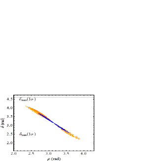
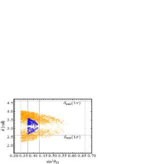
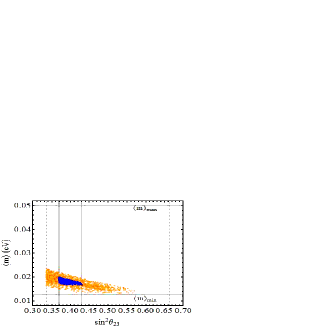
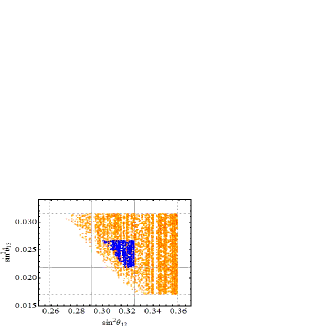
Figure 1: Scatter plots displaying the correlations among some neutrino mass and mixing observables following from Eq. (1). The horizontal and vertical full lines display the $1\sigma$ bounds of Ref. [1] on the corresponding observables; the dashed lines display the $3\sigma$ bounds. The blue (dark) points were found by allowing all the observables to lie within their corresponding $1\sigma$ ranges of Table 1; the yellow (light) points pertain to the $3\sigma$ ranges. $\langle m\rangle_{\rm min}$ and $\langle m\rangle_{\rm max}$ are the minimal and maximal values of the effective mass in the inverted hierarchy with vanishing neutrino mass.

which confirms our analytical expressions. Again, we stress the interesting correlation between the $CP$-violating Dirac phase $\delta$ and the atmospheric neutrino mixing angle $\theta_{23}$.

Next we turn to model realizations of the scenario under study. We shall present three such models. We use the type-I seesaw mechanism with only two right-handed neutrinos $\nu_{R1,2}$; this immediately ensures the existence of one massless neutrino. In the first model we need two Higgs doublets $\phi_{1,2}$ and a complex scalar gauge singlet $S$. Let there be a $\mathbb{Z}_{4}$ symmetry under which the fields—including the left-handed lepton doublets $D_{L\alpha}$ ($\alpha=e,\mu,\tau$)—transform as

$$D_{Le}\to-iD_{Le}\,,\quad D_{L\mu}\to-iD_{L\mu}\,,\quad e_{R}\to-e_{R}\,,\quad\mu_{R}\to-\mu_{R}\,,$$ (15a)

$$\nu_{R1}\to-i\nu_{R1}\,,\quad\phi_{1}\to i\phi_{1}\,,\quad S\to-iS\,.$$ (15b)

The Yukawa couplings $\bar{D}_{Le}\phi_{1}e_{R}$ and $\bar{D}_{L\mu}\phi_{1}\mu_{R}$ give mass to the electron and the muon while $\bar{D}_{L\tau}\phi_{2}\tau_{R}$ gives mass to the $\tau$. The Yukawa couplings to the right-handed neutrinos are

$$\mathcal{L}_{\mathrm{Yukawa}} = -y_{6}\,\bar{\nu}_{R1}C\bar{\nu}_{R2}^{T}\,S-\left(y_{1}\bar{D}_{Le}+y_{2}\bar{D}_{L\mu}\right)\nu_{R1}\,\tilde{\phi}_{2}$$ (16)

$$-\left(y_{4}\bar{D}_{Le}+y_{5}\bar{D}_{L\mu}\right)\nu_{R2}\,\tilde{\phi}_{1}-y_{3}\bar{D}_{L\tau}\,\nu_{R2}\,\tilde{\phi}_{2}+\mathrm{H.c.},$$

where $y_{1\mbox{--}6}$ are coefficients, $C$ is the charge-conjugation matrix in Dirac space, and $\tilde{\phi}_{k}=i\sigma_{2}\phi_{k}^{\ast}$ for $k=1,2$. There is also a bare Majorana mass term

$$\mathcal{L}_{\mathrm{Majorana}}=-\frac{m}{2}\,\bar{\nu}_{R2}\,C\bar{\nu}_{R2}^{T}+\mathrm{H.c.}$$ (17)

Therefore, the neutrino mass matrices, in the notation

$$\mathcal{L}_{\nu\,\mathrm{mass}}=-\bar{\nu}_{R}\,M_{D}\,\nu_{L}-\frac{1}{2}\,\bar{\nu}_{R}\,M_{R}\,C\bar{\nu}_{R}^{T}+\mathrm{H.c.},$$ (18)

are

$$M_{D}=\left(\begin{array}[]{ccc}y_{1}^{\ast}v_{2}&y_{2}^{\ast}v_{2}&0\\ y_{4}^{\ast}v_{1}&y_{5}^{\ast}v_{1}&y_{3}^{\ast}v_{2}\end{array}\right),\quad M_{R}=\left(\begin{array}[]{cc}0&y_{6}s\\ y_{6}s&m\end{array}\right),$$ (19)

where $s=\left\langle 0\left|S\right|0\right\rangle$ and $v_{k}=\left\langle 0\left|\phi_{k}^{0}\right|0\right\rangle$. The effective light-neutrino mass matrix is

$$M = -M_{D}^{T}\,M_{R}^{-1}\,M_{D}$$ (27)

$$= \frac{-1}{y_{6}^{2}s^{2}}\left(\begin{array}[]{cc}y_{1}^{\ast}v_{2}&y_{4}^{\ast}v_{1}\\ y_{2}^{\ast}v_{2}&y_{5}^{\ast}v_{1}\\ 0&y_{3}^{\ast}v_{2}\end{array}\right)\left(\begin{array}[]{cc}-m&y_{6}s\\ y_{6}s&0\end{array}\right)\left(\begin{array}[]{ccc}y_{1}^{\ast}v_{2}&y_{2}^{\ast}v_{2}&0\\ y_{4}^{\ast}v_{1}&y_{5}^{\ast}v_{1}&y_{3}^{\ast}v_{2}\end{array}\right),$$

which evidently has $M_{\tau\tau}=0$.

A simpler model, which dispenses with the singlet $S$, is the following. Let there be a symmetry under which

$$D_{Le}\to\sigma D_{Le}\,\,\quad D_{L\mu}\to\sigma D_{L\mu}\,,\quad D_{L\tau}\to\sigma^{-1}D_{L\tau}\,,$$ (28a)

$$e_{R}\to\sigma^{3}e_{R}\,,\quad\mu_{R}\to\sigma^{3}\mu_{R}\,,\quad\tau_{R}\to\sigma^{-1}\tau_{R}\,,$$ (28b)

$$\nu_{R1}\to\sigma\nu_{R1}\,,\quad\nu_{R2}\to\sigma^{-1}\nu_{R2}\,,\quad\phi_{1}\to\sigma^{-2}\phi_{1}\,.$$ (28c)

where $\left|\sigma\right|=1$ and $\sigma^{4}\neq 1$. Then the Yukawa couplings to the right-handed neutrinos are

$$\mathcal{L}_{\mathrm{\nu\,Yukawa}} = -\left(y_{1}\bar{D}_{Le}+y_{2}\bar{D}_{L\mu}\right)\nu_{R1}\,\tilde{\phi}_{2}$$ (29)

$$-\left(y_{4}\bar{D}_{Le}+y_{5}\bar{D}_{L\mu}\right)\nu_{R2}\,\tilde{\phi}_{1}-y_{3}\bar{D}_{L\tau}\,\nu_{R2}\,\tilde{\phi}_{2}+\mathrm{H.c.},$$

where $y_{1\mbox{--}5}$ are coefficients. There is a bare Majorana mass term

$$\mathcal{L}_{\mathrm{Majorana}}=-m\,\bar{\nu}_{R1}\,C\bar{\nu}_{R2}^{T}+\mathrm{H.c.}$$ (30)

Defining

$$a\equiv y_{1}^{\ast}v_{2}\,,b\equiv y_{2}^{\ast}v_{2}\,,c\equiv y_{3}^{\ast}v_{2}\,,d\equiv y_{4}^{\ast}v_{1}\,,f\equiv y_{5}^{\ast}v_{1}\,,$$ (31)

gives for the mass matrix

$$M=-\frac{1}{m}\left(\begin{array}[]{cc}a&d\\ b&f\\ 0&c\end{array}\right)\left(\begin{array}[]{cc}0&1\\ 1&0\end{array}\right)\left(\begin{array}[]{ccc}a&b&0\\ d&f&c\end{array}\right)=-\frac{1}{m}\left(\begin{array}[]{ccc}2ad&af+bd&ac\\ af+bd&2bf&bc\\ ac&bc&0\end{array}\right).$$ (32)

This $M$ contains five physical parameters,

$$\left|\frac{ad}{m}\right|,\quad\left|\frac{b}{a}\right|,\quad\left|\frac{f}{d}\right|,\quad\left|\frac{c}{d}\right|,\quad\arg{\left(afb^{\ast}d^{\ast}\right)}\,.$$ (33)

These parameters can be computed from the matrix elements of $M$, and thus from the neutrino masses and mixings. Notice for instance that

$$\left|\frac{y_{1}}{y_{2}}\right|=\left|\frac{M_{e\tau}}{M_{\mu\tau}}\right|,\quad\left|\frac{y_{4}}{y_{5}}\right|=\left|\frac{M_{ee}M_{\mu\tau}}{M_{\mu\mu}M_{e\tau}}\right|.$$ (34)

Another example of a model leading to $M_{\tau\tau}=0$ uses $S_{3}$ and $\mathbb{Z}_{3}$ discrete groups as flavour symmetries. The multiplication rules of $S_{3}$ can be found for instance in Ref. [11]. The particle content and group assignments are given in Table 2.

	$\left(D_{Le},D_{L\mu}\right)$	$D_{L\tau}$	$\left(\nu_{R1},\nu_{R2}\right)$	$e_{R}$	$\mu_{R}$	$\tau_{R}$	$\left(\xi_{1},\xi_{2}\right)$	$\chi$
$S_{3}$	$\mathbf{2}$	$\mathbf{1}^{\prime}$	$\mathbf{2}$	$\mathbf{1}$	$\mathbf{1}$	$\mathbf{1}^{\prime}$	$\mathbf{2}$	$\mathbf{1}$
$\mathbb{Z}_{3}$	$1$	$1$	$\omega$	$\omega^{2}$	$\omega$	$1$	$\omega$	$\omega$

Table 2: Field content of our third model. The standard-model Higgs doublet $\phi$, which is invariant under both $S_{3}$ and $\mathbb{Z}_{3}$, has been omitted. The fields $\xi_{1,2}$ and $\chi$ are ‘familons’, i.e. auxiliary scalar gauge singlets. We use $\omega\equiv\exp{\left(i2\pi/3\right)}$.

At leading order in the inverse power of the cutoff scale $\Lambda$, the neutrino Yukawa couplings and the Majorana masses are given by

$$\mathcal{L}_{\nu} = -\frac{g_{1}}{2}\left(\bar{\nu}_{R1}\,C\bar{\nu}_{R1}^{T}\,\xi_{1}^{\ast}+\bar{\nu}_{R2}\,C\bar{\nu}_{R2}^{T}\,\xi_{2}^{\ast}\right)-g_{2}\,\bar{\nu}_{R1}\,C\bar{\nu}_{R2}^{T}\,\chi^{\ast}$$ (35d)

$$-h_{1}\left(\bar{D}_{Le}\,\nu_{R1}+\bar{D}_{L\mu}\,\nu_{R2}\right)\chi^{*}\,\frac{\tilde{\phi}}{\Lambda}$$

$$-h_{2}\left(\bar{D}_{Le}\,\nu_{R2}\,\xi_{1}^{*}+\bar{D}_{L\mu}\,\nu_{R1}\,\xi_{2}^{*}\right)\frac{\tilde{\phi}}{\Lambda}$$

$$-h_{3}\,\bar{D}_{L\tau}\left(\nu_{R1}\,\xi_{1}^{*}-\nu_{R2}\,\xi_{2}^{*}\right)\frac{\tilde{\phi}}{\Lambda}+{\rm H.c.},$$

where $g_{1,2}$ and $h_{1,2,3}$ are dimensionless constants. After $\xi_{1,2}$ and $\chi$ obtain vacuum expectation values according to the alignment [17]

$$\begin{pmatrix}\xi_{1}\\ \xi_{2}\end{pmatrix}\to\begin{pmatrix}\langle\xi_{1}\rangle\\ 0\end{pmatrix},\quad\chi\to\langle\chi\rangle,$$ (36)

and after electroweak symmetry breaking with $v=\langle\tilde{\phi}\rangle$, the mass matrices at low energy take the forms

$$M_{D}=\begin{pmatrix}a&b\\ 0&a\\ c&0\end{pmatrix},\quad M_{R}=\begin{pmatrix}M_{A}&M_{B}\\ M_{B}&0\\ \end{pmatrix},$$ (37)

where $a=h_{1}\langle\chi\rangle^{*}v/\Lambda$, $b=h_{2}\langle\xi_{1}\rangle^{*}v/\Lambda$, $c=h_{3}\langle\xi_{1}\rangle^{*}v/\Lambda$, $M_{A}=g_{1}\langle\xi_{1}\rangle^{\ast}$ and $M_{B}=g_{2}\langle\chi\rangle^{\ast}$. Performing the seesaw diagonalization, one finds the effective Majorana mass matrix

$$M=\frac{1}{M_{B}}\begin{pmatrix}2ab&a^{2}&bc\\ a^{2}&0&ac\\ bc&ac&0\end{pmatrix}-\frac{M_{A}}{M_{B}^{2}}\begin{pmatrix}b^{2}&ab&0\\ ab&a^{2}&0\\ 0&0&0\\ \end{pmatrix}.$$ (38)

The charged-lepton mass sector is written through a combination of higher-dimensional operators and a renormalizable operator. At leading order in $1/\Lambda$, it is given by

$$\mathcal{L}_{l} = -h_{\tau}\bar{D}_{L\tau}\,\tau_{R}\,\phi$$ (39c)

$$-h_{e}\left(\bar{D}_{Le}\,\xi_{1}+\bar{D}_{L\mu}\,\xi_{2}\right)e_{R}\,\frac{\phi}{\Lambda}$$

$$-h_{\mu}\left(\bar{D}_{Le}\,\xi_{2}^{\ast}+\bar{D}_{L\mu}\,\xi_{1}^{\ast}\right)\mu_{R}\,\frac{\phi}{\Lambda}+{\rm H.c.},$$

where $h_{e,\mu,\tau}$ are dimensionless constants. In the vacuum configuration of Eq. (36), the charged-lepton mass matrix is diagonal:

$$M_{l}=\mathrm{diag}\left(\frac{h_{e}}{\Lambda}\,\langle\xi_{1}\rangle,\,\frac{h_{\mu}}{\Lambda}\,\langle\xi_{1}\rangle^{\ast},\,h_{\tau}\right)v^{\ast}.$$ (40)

The hierarchy between $m_{e,\mu}$ and $m_{\tau}$ is naturally explained by the suppression by the cutoff scale.

A dark matter candidate is easily accommodated in this model. For example, we can replace the $S_{3}$ charges of $D_{L\tau}$ and $\tau_{R}$ with $\mathbf{1}$ and introduce a third right-handed neutrino, $\nu_{R3}$, which is $\mathbf{1}^{\prime}$ of $S_{3}$ and $\omega$ of $\mathbb{Z}_{3}$. Then, $\nu_{R3}$ has no Yukawa couplings, so that it is stable. In the early Universe, $\nu_{R3}$ can communicate with the thermal plasma via the $s$-channel exchange of the scalar fields, since it has a $\nu_{R3}\nu_{R3}\chi$ vertex and the real part of $\chi$ mixes with the usual Higgs field. In this setup, it is known [18] that the observed relic density is easily obtained without contradicting the Higgs properties observed at LHC and the direct detection bounds.

In summary, a simple texture-zero scenario can accommodate the values of the $CP$ phase $\delta$ around $\pi$ and of the atmospheric mixing angles $\theta_{23}$ sizably less than $\pi/4$. The framework makes predictions in the form of an inverted hierarchy with a massless neutrino and a strong cancellation in neutrinoless $\beta\beta$ decay. Simple models are possible to realize the scenario.

Acknowledgments

The work of LL is supported through the Marie Curie Initial Training Network “UNILHC” PITN-GA-2009-237920 and also through the projects PEst-OE-FIS-UI0777-2011, PTDC-FIS-098188-2008, and CERN-FP-123580-2011 of the Portuguese FCT. The work of WR was supported by the Max Planck Society through the Strategic Innovation Fund in the project MANITOP.

References

• [1] G. L. Fogli, E. Lisi, A. Marrone, D. Montanino, A. Palazzo, and A. M. Rotunno, Phys. Rev. D 86 (2012) 013012 [arXiv:1205.5254 [hep-ph]].
• [2] D. V. Forero, M. Tórtola, and J. W. F. Valle, Phys. Rev. D 86 (2012) 073012 [arXiv:1205.4018 [hep-ph]].
• [3] M. C. Gonzalez-Garcia, M. Maltoni, J. Salvado, and T. Schwetz, J. High Energy Phys. 1212 (2012) 123 [arXiv:1209.3023 [hep-ph]].
• [4] J. Liao, D. Marfatia, and K. Whisnant, arXiv:1306.4659 [hep-ph].
• [5] C. H. Albright and W. Rodejohann, Eur. Phys. J. C 62 (2009) 599 [arXiv:0812.0436 [hep-ph]].
• [6] P. H. Frampton, S. L. Glashow, and D. Marfatia, Phys. Lett. B 536 (2002) 79 [hep-ph/0201008].
• [7] A. Merle and W. Rodejohann, Phys. Rev. D 73 (2006) 073012 [hep-ph/0603111].
• [8] W.-L. Guo, Z.-Z. Xing, and S. Zhou, Int. J. Mod. Phys. E 16 (2007) 1 [hep-ph/0612033].
• [9] E. I. Lashin and N. Chamoun, Phys. Rev. D 85 (2012) 113011 [arXiv:1108.4010 [hep-ph]].
• [10] P. O. Ludl, S. Morisi, and E. Peinado, Nucl. Phys. B 857 (2012) 411 [arXiv:1109.3393 [hep-ph]].
• [11] W. Rodejohann, M. Tanimoto. and A. Watanabe, Phys. Lett. B 710 (2012) 636 [arXiv:1201.4936 [hep-ph]].
• [12] W. Grimus and P. O. Ludl, JHEP 1212 (2012) 117 [arXiv:1209.2601 [hep-ph]].
• [13] W. Rodejohann, J. Phys. G: Nucl. Part. Phys. 39 (2012) 124008 [arXiv:1206.2560 [hep-ph]].
• [14] G. Drexlin, V. Hannen, S. Mertens, and C. Weinheimer, Adv. High Energy Phys. 2013 (2013) 293986 [arXiv:1307.0101 [physics.ins-det]].
• [15] D. S. Parno, arXiv:1307.5289 [physics.ins-det].
• [16] K. N. Abazajian et al., Astropart. Phys. 35 (2011) 177 [arXiv:1103.5083 [astro-ph.CO]].
• [17] N. Haba and K. Yoshioka, Nucl. Phys. B 739 (2006) 254 [hep-ph/0511108].
• [18] L. Lopez-Honorez, T. Schwetz, and J. Zupan, Phys. Lett. B 716 (2012) 179 [arXiv:1203.2064 [hep-ph]].