Modeling the Evolution and Distribution of the Frequency’s Second Derivative and Braking Index of Pulsar Spin with Simulations

Abstract

We model the evolution of spin frequency’s second derivative $\ddot{\nu}$ and braking index $n$ of radio pulsars with simulations within the phenomenological model of their surface magnetic field evolution, which contains a long-term decay modulated by short-term oscillations. For the pulsar PSR B0329+54, the model can reproduce the main characteristics of its $\ddot{\nu}$ variation with oscillation periods, predicts another $\sim 50$ yr oscillation component and another recent swing of the sign of $\ddot{\nu}$. We show that the “averaged” $n$ is different from the instantaneous $n$, and its oscillation magnitude decreases abruptly as the time span increases, due to the “averaging” effect. The simulation predicted timing residuals agree with the main features of the reported data. We further perform Monte Carlo simulations for the distribution of the reported data in $|\ddot{\nu}|$ versus characteristic age $\tau_{\rm c}$ diagram. The model with a power law index $\alpha=0.5$ can reproduce the slope of the linear fit to pulsars’ distributions in the diagrams of $\log|\ddot{\nu}|-\log\tau_{\rm c}$ and $\log|n|-\log\tau_{\rm c}$, but the oscillations are responsible for the almost equal number of positive and negative values of $\ddot{\nu}$, in agreement with our previous analytical studies; an oscillation period of about several decades is also preferred. However the range of the oscillation amplitudes is $-11.4\lesssim\log f\lesssim-10.2$, slightly lager than the analytical prediction, $\log f\simeq-11.85$, because the “averaging” effect was not included previously.

1 Introduction

The spin-down of radio pulsars is caused by emitting electromagnetic radiation and by accelerating particle winds. Traditionally, the evolution of their rotation frequencies $\nu$ may be described by the braking law

$$\dot{\nu}=-K\nu^{n},$$ (1)

where $n$ is the braking index, $K$ is a positive constant that depends on the magnetic dipole moment and the moment of inertia of the neutron star. By differentiating Equation (1), one can obtain $n$ in terms of observables, $n=\ddot{\nu}\nu/\dot{\nu}^{2}$. For the standard vacuum magnetic dipole radiation model with constant magnetic fields (i.e. $\dot{K}=0$), $n=3$ (Manchester & Taylor 1977). Thus the frequency’s second derivative can be simply expressed as

$$\ddot{\nu}=3\dot{\nu}^{2}/\nu.$$ (2)

The model predicts $\ddot{\nu}>0$ and $|\ddot{\nu}|$ should be very small.

However, unexpectedly large values of $\ddot{\nu}$ were measured for several dozen pulsars thirty years ago (Gullahorn & Rankin 1978; Helfand et al. 1980; Manchester & Taylor 1977), and many of those pulsars surprisingly showed $\ddot{\nu}<0$. Some authors suggested that the observed values of $\ddot{\nu}$ could result from a noise-type fluctuation in the pulsar period (Helfand et al. 1980; Cordes 1980; Cordes & Helfand 1980). Based on the timing data of PSR B0329+54, Demia${\rm\acute{n}}$ski & Pr${\rm\acute{o}}$szy${\rm\acute{n}}$ski (1979) further proposed that a distant planet would influence $\ddot{\nu}$, and the quasi-sinusoidal modulation in timing residuals might be caused by changes in pulse shape, precession of a magnetic dipole axis, or an orbiting planet. Baykal et al. (1999) investigated the stability of $\ddot{\nu}$ of PSR B0823+26, B1706-16, B1749-28 and B2021+51 using their time-of-arrival (TOA) data extending to more than three decades, confirmed that the anomalous $\ddot{\nu}$ terms of these sources arise from red noise (timing residual with low frequency structure), which may originate from the external torques from the magnetosphere of a pulsar.

The relationship between the low frequency structure in timing residuals and the fluctuations in pulsar spin parameters ($\nu$, $\dot{\nu}$, and $\ddot{\nu}$) is very interesting and important. We call both the residuals and the fluctuations as the “timing noise” in the present work, since we will infer that they have the same origin. Timing noise for some pulsars has even been studied over four decades (e.g. Boynton et al. 1972; Groth 1975; Jones 1982; Cordes & Downs 1985; D’Alessandro et al. 1995; Kaspi, Chakrabarty & Steinberger 1999; Chukwude 2003; Livingstone et al. 2005; Shannon & Cordes 2010; Liu et al. 2011; Coles et al. 2011; Jones 2012). However, the origins of the timing noise are still controversial and there is still unmodelled physics to be understood. Boynton et al. (1972) suggested that the timing noise might arise from “random walk” processes. The random walk in $\nu$ may be produced by small scale internal superfluid vortex unpinning (Alpar, Nandkumar & Pines 1986; Cheng 1987a), or short time ($t\sim 10~{}{\rm ms}$ for Crab pulsar) fluctuations in the size of outer magnetosphere gap (Cheng 1987b). Stairs, Lyne & Schemar (2000) reported long time-scale, highly periodic and correlated variations in the pulse shape and the slow-down rate of the pulsar PSR B1828-11, which have generally been considered as evidence of free precession. The possibilities were also proposed that the quasi-periodic modulations in timing residuals could be caused by an orbiting asteroid belt (Cordes & Shannon 2008) or a fossil accretion disk (Qiao et al. 2003).

Recently, Hobbs et al. (2010, hereafer H2010) carried out so far the most extensive study of the long term timing irregularies of 366 pulsars. Besides ruling out some timing noise models in terms of observational imperfections, random walks, and planetary companions, some of their main conclusions are: (1) timing noise is widespread in pulsars and is inversely correlated with pulsar characteristic age $\tau_{\rm c}$; (2) significant periodicities are seen in the timing noise of a few pulsars, but quasi-periodic features are widely observed; (3) the structures seen in the timing noise vary with data span, i.e., more quasi-period features are seen for longer data span and the magnitude of $|\ddot{\nu}|$ for shorter data span is much larger than that caused by magnetic braking of the neutron star; and (4) the numbers of negative and positive $\ddot{\nu}$ are almost equal in the sample, i.e. $N(\ddot{\nu}>0)\thickapprox N(\ddot{\nu}<0)$. Lyne et al. (2010) showed credible evidence that timing noise and $\dot{\nu}$ are correlated with changes in the pulse shapes, and are therefore linked and caused by the changes in the pulsar’s magnetosphere.

Blandford & Romani (1988) re-formulated the braking law of a pulsar as $\dot{\nu}=-K(t)\nu^{3}$, which means that the standard magnetic dipole radiation is still responsible for the instantaneous spin-down of a pulsar, and $\ddot{\nu}\nu/\dot{\nu}^{2}\neq 3$ does not indicate deviation from the dipole radiation model, but means only that $K(t)$ is time dependent. Considering the magnetospheric origin of timing noise as inferred by Lyne et al. (2010), we assume that magnetic field evolution is responsible for the variation of $K(t)$, i.e. $K=AB(t)^{2}$, in which $A=\frac{8\pi^{2}R^{6}\sin\theta^{2}}{3c^{3}I}$ is a constant, $R~{}(\simeq 10^{6}~{}{\rm cm})$, $I~{}(\simeq 10^{45}~{}{\rm g~{}cm^{2}})$, and $\theta~{}(\simeq\pi/2)$ is the radius, moment of inertia, and angle of magnetic inclination of the neutron star, respectively. We can rewrite Equation (2) as

$$\ddot{\nu}=3\dot{\nu}^{2}/\nu+2\dot{\nu}\dot{B}/B.$$ (3)

Since the numbers of negative and positive $\ddot{\nu}$ are almost equal, it should be the case that $B$ quasi-symmetrically oscillates, and usually $|2\dot{\nu}\dot{B}/B|\gg 3\dot{\nu}^{2}/\nu$. Meanwhile, it is noticed that pulsars with $\tau_{\rm c}\lesssim 10^{5}~{}{\rm yr}$ always have $\ddot{\nu}>3\dot{\nu}^{2}/\nu$ (H2010); a reasonable understanding is that their magnetic field decays (i.e. $\dot{B}<0$) dominate the field evolution for these “young” pulsars.

Therefore, Zhang & Xie (2012a, hereafter Paper I) constructed a phenomenological model for the dipole magnetic field evolution of pulsars with a long-term decay modulated by short-term oscillations,

$$B(t)=B_{d}(t)(1+\sum k_{i}\sin(\phi_{i}+2\pi\frac{t}{T_{i}})),$$ (4)

where $t$ is the pulsar’s age, and $k_{i}$, $\phi_{i}$, $T_{i}$ are the amplitude, phase and period of the $i$-th oscillating component, respectively. $B_{d}(t)=B_{0}(t/t_{0})^{-\alpha}$, in which $B_{0}$ is the field strength at the age $t_{0}$, and the index $\alpha\gtrsim 0.5$ (see Paper I for details). Substituting Equation (4) into Equation (1), we get the differential equation describing the the spin frequency evolution of a pulsar as follows

$$\dot{\nu}\nu^{-3}=-AB(t)^{2}.$$ (5)

In paper I, we showed that the distribution of $\ddot{\nu}$ and the inverse correlation of $\ddot{\nu}$ versus $\tau_{c}$ could be well explained with analytic formulae derived from the phenomenological model. In Zhang & Xie (2012b, hereafter Paper II), we also derived an analytical expression for the braking index ($n$) and pointed out that the instantaneous value of $n$ of a pulsar is different from the “averaged” $n$ obtained from the traditional phase-fitting method over a certain time span. However, this “averaging” effect was not included in our previous analytical studies; this work is focused on addressing this effect.

This paper is organized as follows. In Section 2, we show that the timescales of magnetic field oscillations are tightly connected to the $\ddot{\nu}$ evolution and the quasi-periodic oscillations appearing in the timing residuals, and the reported data of pulsar B0329+54 are fitted. In Section 3, we perform Monte Carlo simulations on the pulsar distribution in the $\ddot{\nu}-\tau_{\rm c}$ and $n-\tau_{\rm c}$ diagram. Our results are summarized and discussed in Section 4.

2 Modeling the $\ddot{\nu}$ and $n$ Evolution and Timing Residuals of Pulsar B0329+54

PSR B0329+54 is a bright (e.g. 1500 mJy at 400 MHz), $0.71$ s pulsar that had been suspected to possess planetary-mass companions (Demia${\rm\acute{n}}$ski & Pr${\rm\acute{o}}$szy${\rm\acute{n}}$ski 1979; Bailes, Lyne, & Shemar 1993; Shabanova 1995). However the suspected companions have not been confirmed and are currently considered doubtful (Cordes & Downs 1985; Konacki et al. 1999; H2010). Konacki et al. (1999) suggested that the observed ephemeral periodicities of the timing residuals for PSR B0329+54 are intrinsic to this neutron star. H2010 believed that the timing residual has a similar form to the other pulsars in their sample. They plotted $|\ddot{\nu}|$ obtained from the B0329+54 data sets with various time spans (see Figure 12 in their paper). For data spanning $\sim 10$ yr, they measured a large and significant $\ddot{\nu}$, and found that the timing residual takes the form of a cubic polynomial. However, no cubic term was found for data spanning more than $\sim 25$ yr, and $|\ddot{\nu}|$ became significantly smaller. The reported periods of the timing residuals for PSR B0329+54 are $1100~{}{\rm days}$, $2370~{}{\rm days}$, and/or $16.8~{}{\rm years}$ (Demia${\rm\acute{n}}$ski & Pr${\rm\acute{o}}$szy${\rm\acute{n}}$ski 1979; Bailes, Lyne, & Shemar 1993; Shabanova 1995). Here we neglect the two short-period oscillation components, since they have little impact on $|\ddot{\nu}|$ variation due to their relative small oscillation magnitude (Shabanova 1995).

In order to model the $\ddot{\nu}$ evolution for pulsar B0329+54, we firstly obtain $\nu(t)$ by integrating the spin-down law described as Equations (5) and (4) with $\alpha=0.5$, and then the phase

$$\Phi(t)=\int_{t_{0}}^{t}\nu(t^{\prime}){\rm d}t^{\prime}.$$ (6)

Finally, these observable quantities, $\nu$, $\dot{\nu}$ and $\ddot{\nu}$ can be obtained by fitting the phases to the third order of its Taylor expansion over a time span $T_{\rm s}$,

$$\Phi(t_{i})=\Phi_{0}+\nu(t_{i}-t_{0})+\frac{1}{2}\dot{\nu}(t_{i}-t_{0})^{2}+\frac{1}{6}\ddot{\nu}(t_{i}-t_{0})^{3}.$$ (7)

We thus get $\nu$, $\dot{\nu}$ and $\ddot{\nu}$ for $T_{\rm s}$ from fitting to Equation (7), with a certain time interval of phases $\Delta T_{\rm int}=10^{6}~{}{\rm s}$ (interval between each TOA, i.e. $\Delta T_{\rm int}=t_{i+1}-t_{i}$).

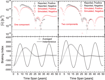
Figure 1: $|\ddot{\nu}|$ and $n$ for PSR B0329+54. Upper panels: $|\ddot{\nu}|$ obtained using different data spans ($T_{s}$). The values reported by H2010 are represented by large cross symbols ($\ddot{\nu}>0$) and large circles ($\ddot{\nu}<0$); our simulated values are represented by small cross symbols ($\ddot{\nu}>0$) and small circles ($\ddot{\nu}<0$); the horizontal dashed line represents $\ddot{\nu}=3\dot{\nu}^{2}/\nu$. Bottom panels: instantaneous (solid lines) and averaged (circles) values of $n$. Left panels: simulation with one oscillation component of $k=3\times 10^{-4}$, $T=16.8~{}{\rm yr}$ and $\phi=3.7$. Right panels: simulation with two oscillation components of $k_{1}=3.3\times 10^{-4}$, $k_{2}=1.8\times 10^{-4}$, and $T_{1}=16.8~{}{\rm yr}$, $T_{2}=50~{}{\rm yr}$, and $\phi_{1}=3.9$, $\phi_{2}=4.0$. The horizontal dotted line represents $n=0$.

In the upper panels of Figure 1, we show the reported and simulated results of $|\ddot{\nu}|$ for various $T_{\rm s}$ for PSR B0329+54. The reported data are read from Figure 12 of H2010. The simulated results with one oscillation component with fitting parameters $k=3\times 10^{-4}$, $T=16.8~{}{\rm yr}$ and $\phi=3.7$ are shown in the left panels, and two oscillation components with $k_{1}=3.3\times 10^{-4}$, $k_{2}=1.8\times 10^{-4}$, $T_{1}=16.8~{}{\rm yr}$, $T_{2}=50~{}{\rm yr}$, and $\phi_{1}=3.9$, $\phi_{2}=4.0$ are shown in the right panels. Besides the $16.8$ yr component, there is another oscillation component with period $\sim 50$ yr in the two component model. In the bottom panels of Figure 1, we show the corresponding $n$ with the same oscillation parameters obtained above. The braking index $n=\ddot{\nu}\nu/\dot{\nu}^{2}$ obtained directly from Equation (5) is called “instantaneous” $n$; similarly that the obtained by fitting phase sets to Equation (7) is called “averaged” $n$. It can be seen that the averaged $n$ has the same variation trends with $\ddot{\nu}$, since $|\Delta\nu/\nu|\sim 10^{-6}$ and $|\Delta\dot{\nu}/\dot{\nu}|\sim 10^{-3}$ are tiny, compared to $|\Delta\ddot{\nu}/\ddot{\nu}|\sim 1$. The magnitude of the first period of the averaged $n$ is close to the instantaneous one, but it decays significantly due to the “averaging” effect.

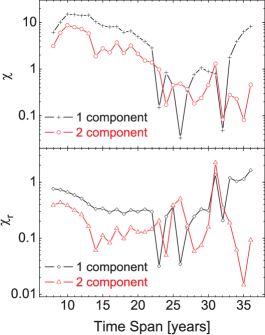
Figure 2: Two goodness of fit parameters $\chi$ and $\chi_{\rm r}$ for the fits of $|\ddot{\nu}|$ variation. It is shown that the two component case is apparently a better fit.

We adopt two goodness of fit parameters to show how well the model matches the data, i.e. $\chi=|\frac{\ddot{\nu}_{\rm M}-\ddot{\nu}_{\rm D}}{\sigma}|$ and $\chi_{\rm r}=|\frac{\ddot{\nu}_{\rm M}-\ddot{\nu}_{\rm D}}{\ddot{\nu}_{\rm M}}|$, where the subscripts ‘M’ and ‘D’ refer to the model results and the reported data, respectively, $\sigma$ the uncertainties of reported data. $\chi$ and $\chi_{\rm r}$ are shown in Figure 2. One can see that both fits are not very good and are certainly rejected by $\chi^{2}$ test. However, we stress that both the one and two component models can reproduce the main characteristics of $\ddot{\nu}$ variation, including the swings between $\ddot{\nu}>0$ and $\ddot{\nu}<0$. On the other hand, the calculated $\chi$ and $\chi_{\rm r}$ apparently indicate that the two component case is a better fit. Unfortunately, we cannot provide any physical information about the links between the identified periodicities, since the physical processes of the oscillations are poorly understood presently.

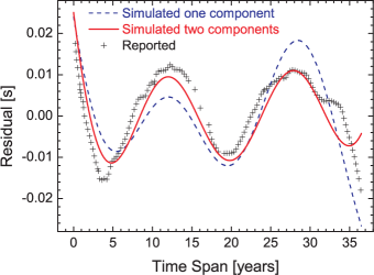
Figure 3: Timing residual of PSR B0329+54. The reported timing residual, after subtraction $\nu$ and $\dot{\nu}$ of the pulsar over the $36.5$ years, is represented by cross symbols. The simulated results with one and two components are represented by dashed and solid lines, respectively. The model parameters are identical with that for the $\ddot{\nu}$ simulation, shown in Figure 1.

The timing residual, after subtraction of the pulsar’s $\nu$ and $\dot{\nu}$ over $36.5$ years for PSR B0329+54, is also simulated with exactly the same model parameters used for modeling $\ddot{\nu}$. In the simulation, the following steps are taken:

(i) We get the model-predicted TOAs with $\Delta T_{\rm int}=10^{6}~{}{\rm s}$ using Equation (6) over $36.5~{}{\rm yr}$, with the same model parameters used for modeling $\ddot{\nu}$.

(ii) By fitting the TOA set $\{\Phi(t_{i})\}$ to

$$\Phi(t)=\Phi_{0}+\nu_{0}(t-t_{0})+\frac{1}{2}\dot{\nu}_{0}(t-t_{0})^{2},$$ (8)

we get $\Phi_{0}$, $\nu_{0}$ and $\dot{\nu}_{0}$.

(iii) Then the timing residual after the subtraction of $\nu$ and $\dot{\nu}$ can be obtained by

$$T_{\rm res}(t_{i})=\frac{\Phi(t_{i})-(\Phi_{0}+\nu_{0}(t_{i}-t_{0})+\frac{1}{2}\dot{\nu}_{0}(t_{i}-t_{0})^{2})}{\nu_{0}}.$$ (9)

In Figure 3, we plot the reported timing residual (from Figure 3 of H2010) with cross symbols and the simulated results for one oscillation component and two components with dashed and solid lines, respectively. Note that the simulated results are not fits of the models to the reported timing residuals; the model parameters are set after many rounds of trials and comparisons with the reported data. One can see that the two-component model matches the observed data better than the one-component model. Our model implies that the timing residual is also caused by the magnetic field oscillation, and the quasi-periodic structures in timing residuals have the same origin (which is determined by Equation (5)) with those in $\ddot{\nu}$, $\dot{\nu}$, and $\nu$ variations.

In general, the two-component model describes the variation of $\ddot{\nu}$ and timing residuals of PSR B0329+54 more precisely than the one-component model. However, the oscillation component with $50$ years period cannot be tested directly from the power spectrum of its timing residuals, since the period is longer than the observational data span. However, there are still some features demonstrating its existence. For instance, the observed data are reported about four years ago, and the two-component model predicts that $\ddot{\nu}$ of the pulsar is now experiencing another switch from positive to negative (as shown in Figure 1), which can be tested with the latest observed data. The test could also be conducted by applying the model to a larger set of pulsars, which have short oscillation periods (shorter than the observed time span), and relatively large oscillation amplitudes (so that the swing behavior of $\ddot{\nu}$ could emerge; the exact criteria of $k$ depend on $\nu$, $\dot{\nu}$ and $T$).

3 Simulating the Distribution of $\ddot{\nu}$ and its Correlation with $\tau_{\rm c}$

We show the measured $|\ddot{\nu}|$ versus $\tau_{\rm c}$ for $341$ normal radio pulsars with $\tau_{\rm c}<10^{9}~{}{\rm yr}$ in Figure 4 (the reported data are obtained from Table 1 of H2010). The linear fits for $\log|\ddot{\nu}|~{}[10^{-24}~{}{\rm s^{-3}}]=a+b\log\tau_{c}~{}[{\rm yr}]$ are given. It is found that the slope $b$ for $\tau_{\rm c}<10^{6}~{}{\rm yr}$ ($b_{1}=-2.0$) is obviously steeper than that for $\tau_{\rm c}>10^{6}~{}{\rm yr}$ ($b_{2}=-1.1$) for $\ddot{\nu}>0$; the latter is slightly steeper than the slope for $\ddot{\nu}<0$ ($b_{3}=-0.94$). It was found that $b_{1}$ is caused by the magnetic field decay, which dominates the field evolution for young pulsars with $\tau_{\rm c}\lesssim 10^{6}~{}{\rm yr}$ (Paper I). In this section, based on our phenomenological model, we use the Monte Carlo method to simulate the distributions of $\ddot{\nu}$ and $n$, and their correlation with $\tau_{\rm c}$.

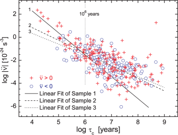
Figure 4: The reported $|\ddot{\nu}|$ versus characteristic age $\tau_{\rm c}$. The reported data are obtained from Table 1 of H2010. The crosses and circles indicate $\ddot{\nu}>0$ and $\ddot{\nu}<0$, respectively. The solid line indicates the linear fit for $\ddot{\nu}>0$ and $\tau_{\rm c}<10^{6}~{}{\rm yr}$ (sample 1), the dashed line indicates the linear fit for $\ddot{\nu}>0$ and $10^{6}~{}{\rm yr}<\tau_{\rm c}<10^{8}~{}{\rm yr}$ (sample 2), and the dotted line indicates the linear fit for $\ddot{\nu}<0$ and $\tau_{\rm c}<10^{8}~{}{\rm yr}$ (sample 3). The vertical line indicates $\tau_{\rm c}=10^{6}~{}{\rm yr}$.

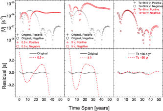
Figure 5: The effects of $\nu$, $\dot{\nu}$ and $T_{\rm s}$ on $\ddot{\nu}$ and timing residuals. The results for different $\nu$ ($\nu$ and $0.5\nu$) are shown in the left panels, the results of different $\dot{\nu}$ ($\dot{\nu}$ and $5\dot{\nu}$) are shown in middle panels, and the results of different $T_{\rm s}$ (36.5 yr and 50 yr) are shown in left panels.

3.1 Determining the Sample Space

We firstly check the effects of the variations of $\nu$, $\dot{\nu}$ and $T_{\rm s}$ on $\ddot{\nu}$ and timing residuals. We still adopt the two component model of PSR B0329+54 and the same model parameters obtained above. Based on the model, we show $|\ddot{\nu}|$ and timing residuals for different values of $\nu$, $\dot{\nu}$ and $T_{\rm s}$ in Figure 5. In the left panels of Figure 5, one can see that both $|\ddot{\nu}|$ and timing residuals for $0.5\nu$ ($\nu$ is the pulsar’s reported value, and other parameters are fixed to their reported values) are apparently larger than that of $\nu$. The results are similar for the case of $5\dot{\nu}$ in the middle panels. In the right panels, one can see that $\ddot{\nu}$ and the timing residuals have very small changes for $T_{\rm s}=36.5$ yr and $50$ yr, thus the results are not sensitive to $T_{\rm s}$. We therefore need to determine the sample space well for $\nu$ and $\dot{\nu}$, but only approximately for $T_{\rm s}$.

The distribution of $\nu$ can be well described by a lognormal distribution, as shown in Figure 6(a). The best-fit parameter set is $(x_{\rm c},\sigma)=(0.66,0.78)$, where $x_{\rm c}$ and $\sigma$ are the mean and standard deviation, respectively. In the simulation, we choose the same distribution as the sample space for $\nu$ with $(x_{\rm c},\sigma)=(0.67,0.86)$. We show about 3500 sample outcomes in Figure 6(b), and their best-fit parameter set $(0.66,0.85)$ approximately equals the set of the reported sample after the selection effect of the “death line” is included. The theoretical “death line” we adopt here is $7\log B-13\log P=78$ (Chen & Ruderman 1993), where the dipole magnetic field $B$ is in units of Gauss and period $P$ is in units of seconds. For different simulated samples, the best-fit parameter sets have small fluctuations that can be ignored.

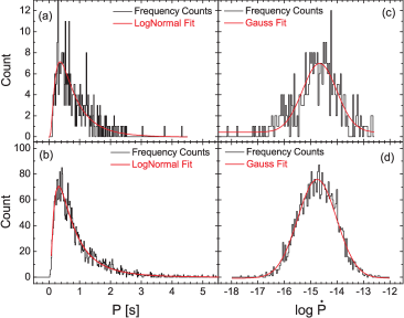
Figure 6: Distributions and fits for $\nu$ and $\log\dot{\nu}$. (a) Distribution of $\nu$ for the reported sample and their lognormal fit. (b) Distribution of $\nu$ for the simulated sample and their lognormal fit; the selection effect of “death line” is included for the sample space. (c) Distribution of $\log\dot{\nu}$ for the reported sample and their Gauss fit. (d) Distribution of $\log\dot{\nu}$ for the simulated sample and their Gauss fit; the selection effect of “death line” is included for the sample space.

The distribution of $\log\dot{\nu}$ can be well described by a Gaussian distribution, as shown in Figure 6(c). The best-fit parameter set is $(\mu,\sigma)=(-14.66,1.3)$, in which $\mu$ and $\sigma$ are the mean and standard deviation, respectively. Similarly, the parameter set $(-14.8,0.7)$ is adopted for the sample space, and the best-fit parameter set $(-14.75,1.47)$ for the 3500 sample outcomes approximately equals the set of the reported sample after the selection effect of the “death line” is considered, as shown in Figure 6(d).

We plot the $P-\log\dot{P}$ diagram for the reported sample and the contour lines of the $\sim 3500$ simulated sample outcomes in Figure 7, in which the period $P=1/\nu$. One can see that the simulated sample agrees with the reported sample very well, about $93\%$ of the reported data are covered by the $2\sigma$ area of the simulated data and $62\%$ of the reported data are covered by the $1\sigma$ area.

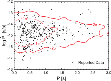
Figure 7: The reported data points and contour lines for the $\sim 3500$ simulated sample outcomes in the $P-\log\dot{P}$ diagram. The $1\sigma$ line (dash-dotted line) indicates the area covering $\sim 68\%$ sample outcomes, and $2\sigma$ line (solid line) indicates the area of $\sim 95\%$ sample outcomes.

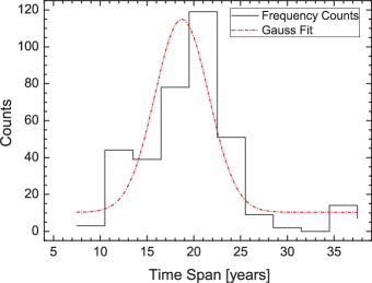
Figure 8: Histogram of the time spans of H2010 observations and its Gaussian fit.

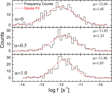
Figure 9: Histograms of the oscillation parameter $f$ and their Gaussian fits for different long-term magnetic field decay index ($\alpha$).

The histogram of the time spans of observations $T_{\rm s}$ (H2010) and its Gaussian fit are shown in Figure 8. The best-fit parameter set $(\mu,\sigma)$ is $(18.7~{}{\rm yr},5.76~{}{\rm yr})$, which determines the sample space for the upper limit of Equation (6). Though the distribution of $T_{\rm s}$ is poorly modelled by the Gaussian, it is still good enough for the simulation, since $\ddot{\nu}$ and timing residuals are not sensitive to $T_{\rm s}$, as shown in the right panels of Figure 5.

From Equation (5), we obtained the analytic approximation (in Paper I) for $\ddot{\nu}$

$$\ddot{\nu}\simeq-2\dot{\nu}(\alpha/t\pm f),$$ (10)

where $f=2\pi k/T$ represents the magnitude of the oscillation term. Thus, both parameters $k$ and $T$ are important. In our previous work (Paper I), we get $\log f$ for all pulsars in the sample of H2010 by the following steps: (a) we set $\alpha=0$, $0.5$ or $1.0$; (b) for a certain value of $\alpha$, we can get $\eta$ by fitting the data of young pulsars with $\tau_{c}<2\times 10^{6}~{}{\rm yr}$ to Equation (15) in Paper I, where $\eta$ is defined as $\eta=(3.3\times 10^{19}/B_{0})^{1/\alpha}2\alpha/t_{0}$; (c) then $f$ can be obtained by substituting $\nu$, $\dot{\nu}$ and $\ddot{\nu}$ of each pulsar into Equation (14) (in Paper I). One can see that the distribution of $\log f$ shows a single peak for a certain $\alpha$ (see Figure 8 in Paper I). We show the distributions for different values of $\alpha$ and their Gaussian fits in Figure 9. The fitted parameter set $(\mu,\sigma)$ is $(-12.04,1.45)$, $(-11.85,1.23)$ and $(-11.86,1.05)$ for $\alpha=0$, $0.5$ and $1.0$, respectively. If we assume that the period $T$ of magnetic field oscillations is a constant, the sample space parameters of $k$ can be obtained from $k=fT/2\pi$.

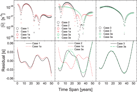
Figure 10: Comparisons of $\ddot{\nu}$ and timing residuals with one oscillation component and two oscillation components. The model of B0329+54 is still adopted. Case 1a: one oscillation component with $k=3\times 10^{-4}$ and $T=16.8~{}{\rm yr}$. Case 1: two oscillation components with $k_{1}=3\times 10^{-4}$, $T_{1}=16.8~{}{\rm yr}$ (the short period is the dominating component), and $k_{2}=3\times 10^{-5}$, $T_{2}=50~{}{\rm yr}$. Case 2: two oscillation components with $k_{1}=3\times 10^{-4}$, $T_{1}=16.8~{}{\rm yr}$, and $k_{2}=3\times 10^{-4}$, $T_{2}=50~{}{\rm yr}$ (no dominating component). Case 3a: one oscillation component with $k=3\times 10^{-4}$ and $T=50~{}{\rm yr}$. Case 3: two oscillation components with $k_{1}=3\times 10^{-5}$, $T_{1}=16.8~{}{\rm yr}$ and $k_{2}=3\times 10^{-4}$, $T_{2}=50~{}{\rm yr}$ (the long period is the dominating component).

Sometimes it might be necessary to take multiple oscillation components, since multiple peaks are often seen in the power spectra of the timing residuals of many pulsars (H2010). However, to our knowledge there is not any statistical data on the numbers of the oscillation components as well as their periods reported up to now in the literature. For simplicity, here we assume that there is always a dominating oscillation component (Paper I), which mainly determines the variations of $\ddot{\nu}$ and the timing residuals. In Figure 10, we compare $\ddot{\nu}$ and the timing residuals between the two component and the one component case. It is found that if one of the components dominates, the two component model can be well approximated by the one component model which has the same $k$ and $T$ as the dominating one. However, if the two components have comparable $k$, the approximation is no longer valid (as shown in the middle panels), and some uncertainties may be introduced, which we have to live with currently. In addition, since $T$ is also not well known to date, we will try several different values for it in the following Monte Carlo simulations.

3.2 Results of Monte Carlo Simulations

One can draw a set of $\nu$, $\dot{\nu}$, $T_{\rm s}$, $T$, $k$, and $\phi$ from the above sample space. The sample of the phase $\phi$ of the field oscillation follows a uniform random distribution in the range of $0$ to $2\pi$. With these quantities and a corresponding start time $t_{0}$, we can obtain a rotation phase set $\{\Phi(t_{i})\}$ using Equation (6). In the calculation, the time interval of TOAs is also assumed as a constant, i.e. $\Delta T_{\rm int}=10^{6}~{}{\rm s}$. Then the “averaged” values of $\nu$, $\dot{\nu}$ and $\ddot{\nu}$ can be obtained by fitting $\{\Phi(t_{i})\}$ to Equation (7). Hence one has its $|\ddot{\nu}|$ and $\tau_{\rm c}$. Repeat this procedure for $N$ times, we will have $N$ data points in the $|\ddot{\nu}|$-$\tau_{\rm c}$ diagram. In Table 1 we summarize all the model parameters and results of simulations.

3.2.1 Effects of power-law decay index

Case I: no long-term decay, i.e. $\alpha=0$. For this case, we assume $B_{0}=3.2\times 10^{19}\sqrt{-\dot{\nu}/\nu^{3}}$ and $t_{0}=-\nu/2\dot{\nu}$, and the oscillation period $T=20~{}{\rm yr}$. We plot the simulated results in the upper four panels of Figure 11. The number of the total data points is $N_{\rm total}=3350$ (the number is not fixed for each simulation, due to the selection effect of “death line”), in which the numbers of positive and negative $\ddot{\nu}$ are $N_{\rm p}=1813$ and $N_{\rm n}=1537$, respectively. The distribution contours and the reported data are also shown for $\ddot{\nu}>0$ and $\ddot{\nu}<0$, respectively. For $\ddot{\nu}>0$ about $94\%$ and $63\%$ of the reported data are covered by the $2\sigma$ and $1\sigma$ areas of the simulated data, respectively; similarly, for $\ddot{\nu}<0$ about $94\%$ and $73\%$ of the reported data are covered by the $2\sigma$ and the $1\sigma$ areas, respectively. However, the steep slope for the young pulsars with $\tau_{\rm c}<10^{6}~{}{\rm yr}$ cannot be well reproduced.

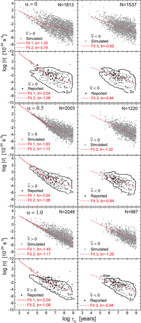
Figure 11: Simulations of the $|\ddot{\nu}|$-$\tau_{\rm c}$ distribution in the cases of no long-term magnetic field decay ($\alpha=0$, the upper four panels), moderate long term magnetic field decay ($\alpha=0.5$, the middle four panels), and strong long term magnetic field decay ($\alpha=1$, the bottom four panels). Linear fit 1: for $\ddot{\nu}>0$ with $\tau_{\rm c}<10^{6}~{}{\rm yr}$ (young pulsars); Linear fit 2: for $\ddot{\nu}>0$ with $10^{6}~{}{\rm yr}<\tau_{\rm c}<10^{8}~{}{\rm yr}$ (old pulsars); Linear fit 3: for $\ddot{\nu}<0$ with $\tau_{\rm c}<10^{8}~{}{\rm yr}$. The best-fit slopes ($b$) for all simulations and reported data are labelled in these corresponding panels.

Case II: power-law decay with $\alpha=0.5$. For this case, we assume $t_{0}=H_{1}/B_{0}^{2}$, where $H_{1}=3.075\times 10^{36}~{}({\rm G^{2}s})$ is obtained by the best-fit for the reported young pulsars with $\tau_{\rm c}>10^{6}~{}{\rm yr}$ and $\ddot{\nu}>0$ (Paper I), and $T=20~{}{\rm yr}$. We plot the simulated results in the middle four panels of Figure 11. $N_{\rm total}=3223$, in which $N_{\rm p}=2003$ and $N_{\rm n}=1220$, respectively. $N_{\rm p}/N_{\rm total}$ ($\sim 62\%$) is larger than the reported $\sim 54\%$. For $\ddot{\nu}>0$ about $95\%$ and $74\%$ of the reported data are covered by the $2\sigma$ and $1\sigma$ areas of the simulated data, respectively; similarly, for $\ddot{\nu}<0$ about $88\%$ and $63\%$ of the reported data are covered by the $2\sigma$ and the $1\sigma$ areas, respectively. Notably, a steeper slope for the young pulsars with $\tau_{\rm c}<10^{6}~{}{\rm yr}$ can almost be reproduced.

Case III: power-law decay with $\alpha=1.0$. For this case, we assume $t_{0}=H_{2}/B_{0}^{2}$, where $H_{2}=5.16\times 10^{24}~{}({\rm G~{}s})$ is also obtained by the best-fit for the reported young pulsars with $\tau_{\rm c}>10^{6}~{}{\rm yr}$ and $\ddot{\nu}>0$ (Paper I), and $T=20~{}{\rm yr}$. We plot the simulated results in the bottom four panels of Figure 11. $N_{\rm total}=3235$, in which $N_{\rm p}=2248$ and $N_{\rm n}=987$, respectively. $N_{\rm p}/N_{\rm total}$ is larger than $69\%$. For $\ddot{\nu}>0$, about $81\%$ of the reported data are covered by the $2\sigma$ area of the simulated data, but only $34\%$ of the reported data are covered by $1\sigma$ area; for $\ddot{\nu}<0$ about $90\%$ and $55\%$ of the reported data are covered by the $2\sigma$ and the $1\sigma$ areas, respectively. However, the slope for the young pulsars with $\tau_{\rm c}<10^{6}~{}{\rm yr}$ is still not steep enough.

In conclusion, it is found that $\alpha=0.5$ is favored by the reported data.

Table 1: Summary for all the simulated results. The first row lists the reported data in our sample. The numbers in the left and rights parts of brackets correspond to $\ddot{\nu}>0$ and $\ddot{\nu}<0$, respectively.

	Model Parameters					Results					Note
	$\alpha$	$\log f$	$k~{}(10^{-4})$	$T$ (yr)	$(N_{\rm p},N_{\rm n})$	$b_{1}$	$b_{2}$	$b_{3}$	$1\sigma~{}($%$)$	$2\sigma$ ($\%$)
	–	–	–	–	(183, 158)	-2.04	-1.08	-0.94	–	–	Fig 4
	0.0	-12.04	0.92	20	(1813, 1537)	-1.35	-0.79	-0.92	(94, 94)	(63, 73)	Fig 11
	0.5	-11.85	1.42	20	(2003, 1220)	-1.83	-1.13	-1.22	(95, 88)	(74, 63)	Fig 11
	1.0	-11.86	1.38	20	(2248,  987)	-1.45	-1.17	-1.25	(95, 88)	(74, 63)	Fig 11
	0.0	-12.04	0.23	5	(2061, 1099)	-1.09	-1.75	-1.82	–	–	Fig 12
	0.5	-11.85	0.35	5	(2669,  611)	-1.93	-1.99	-1.82	–	–	Fig 12
	1.0	-11.86	0.35	5	(2580,  386)	-1.49	-1.31	-1.26	–	–	Fig 12
	0.0	-12.04	4.58	100	(1598, 1510)	-1.41	-0.79	-0.96	–	–	Fig 12
	0.5	-11.85	7.09	100	(2140, 1303)	-1.71	-1.12	-1.29	–	–	Fig 12
	1.0	-11.86	6.93	100	(1948, 1459)	-1.15	-0.85	-0.95	–	–	Fig 12
	0.5	-11.85	70.9	$10^{3}$	(2039, 1438)	-1.20	-1.03	-1.24	–	–	Fig 13
	0.5	-11.85	709.0	$10^{4}$	(2306, 1463)	-1.25	-1.21	-1.07	–	–	Fig 13
	0.5	-11.85	7090	$10^{5}$	(2581,  954)	-1.54	-1.21	-1.04	–	–	Fig 13
	0.5	-11.35	6.73	$30$	(1950, 1681)	-1.72	-0.84	-1.03	(93, 90)	(69, 66)	Fig 15

3.2.2 Effects of Oscillation Period

The case of $T=5~{}{\rm yr}$. We keep all parameters the same as those in the above subsection, except that the oscillation period is changed to $5~{}{\rm yr}$. The main results are shown in the upper six panels of Figure 12. One can see that $N_{\rm p}\gg N_{\rm n}$. It can be inferred that the oscillation has impacts mainly on older pulsars, since $\ddot{\nu}<0$ appears mostly in the area with larger $\tau_{\rm c}$. The slopes (i.e. $b$) for the young pulsars with $\ddot{\nu}>0$ are too flat, but the slopes for the old $\ddot{\nu}>0$ and $\ddot{\nu}<0$ are too steep. In addition, one can see that there is a crowded area of data points along the lower boundary for $\ddot{\nu}>0$. The crowded area is caused by the underestimation for $|\ddot{\nu}|$, because the “averaging” effect is strong when the oscillation period is much shorter than the observation time span. However, there is no such crowded area in the reported data, which indicates that the period $T=5~{}{\rm yr}$ is too short for most pulsars in the sample. Simulations show that there is no obvious crowded area when the mean value of period is longer than thirty years, i.e. $T\gtrsim 30~{}{\rm yr}$, which is actually beyond the $2\sigma$ range of the sample space for the observation time span, and thus the “averaging” effect does not dominate the reported $\ddot{\nu}$.

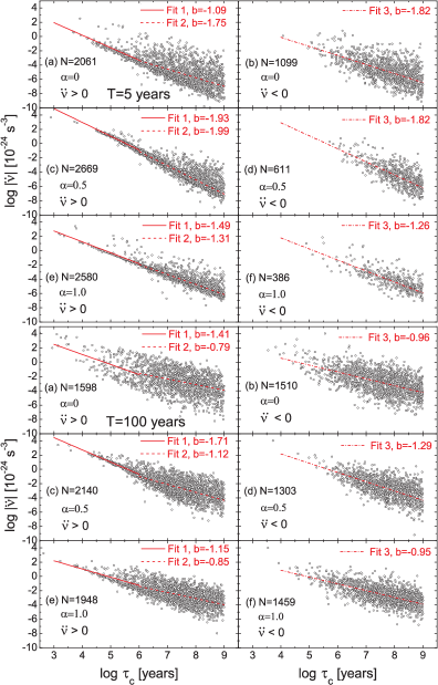
Figure 12: Simulations of the $|\ddot{\nu}|$-$\tau_{\rm c}$ distribution for different combinations of long-term magnetic field decay index ($\alpha$) and the period $T$, as marked in each panel. Fit 1: for $\ddot{\nu}>0$ with $\tau_{\rm c}<10^{6}~{}{\rm yr}$ (young pulsars); Fit 2: for $\ddot{\nu}>0$ with $10^{6}~{}{\rm yr}<\tau_{\rm c}<10^{8}~{}{\rm yr}$ (old pulsars); Fit 3: for $\ddot{\nu}<0$ with $\tau_{\rm c}<10^{8}~{}{\rm yr}$. $N$ is the number of data points.

The case of $T=100~{}{\rm yr}$. We keep all parameters the same but the oscillation period is changed to $100~{}{\rm yr}$. We show the simulated results in the lower six panels of Figure 12. It is found that $N_{\rm p}\approx N_{\rm n}$ for $\alpha=0$. But for the cases of $\alpha=0.5$ and $\alpha=1.0$, $N_{\rm p}\gg N_{\rm n}$ ($N_{\rm p}/N_{\rm total}=62\%$ and $57\%$, respectively). As expected by the above analysis, there is not a clear crowded area for this case. The steep slope ($b$) for the young pulsars with $\ddot{\nu}>0$ can only be reproduced by $\alpha=0.5$; this suggests again that $\alpha=0.5$ dominates the long-term magnetic field decay for young pulsars with $\tau_{\rm c}<10^{6}~{}{\rm yr}$.

The cases of $T=10^{3},10^{4}$ and $10^{5}~{}{\rm yr}$. The results of simulations for $T=10^{3},10^{4}$ and $10^{5}~{}{\rm yr}$ are shown in Figure 13. One can see that there are many simulated data points spread over from $\tau_{c}=10^{5}$ to $10~{}{\rm yr}$ as shown in the left panels for $\ddot{\nu}>0$, which is apparently different from reported data. For the reported data and simulated data of $T\lesssim 100~{}{\rm yr}$, the overall shape of data points is a triangle like; as the period increases from $T=10^{3}$ to $10^{5}~{}{\rm yr}$, the overall shape of data points gradually becomes a band like. This is due to the oscillation parameter $k\gtrsim 1$ for $T=10^{4}~{}{\rm yr}$ (since $f$ is fixed and $k=fT/2\pi$), and such a large oscillation magnitude will deviate the $\dot{\nu}$ from its initial value significantly, which is inconsistent with the observational facts that $\dot{\nu}$ does not change significantly. Thus the simulations can give a constraint for the upper limit of oscillation period, $T\lesssim 10^{3}~{}{\rm yr}$.

In conclusion, $T$ has an influence on the distribution density and the overall shape of simulated data points when $f$ is a constant. By comparing the distribution density and the overall shape with the reported data, we give a rough constraint for the oscillation period, $30~{}{\rm yr}\lesssim T\lesssim 1000~{}{\rm yr}$.

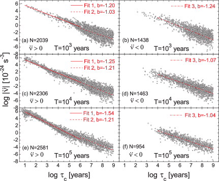
Figure 13: Simulations of the $|\ddot{\nu}|$-$\tau_{\rm c}$ distribution in the cases of moderate long term magnetic field decay ($\alpha=0.5$) for long oscillation period, $T=10^{3}$, $10^{4}$ and $10^{5}~{}{\rm yr}$. Linear fit 1: for $\ddot{\nu}>0$ with $\tau_{\rm c}<10^{6}~{}{\rm yr}$; Linear fit 2: for $\ddot{\nu}>0$ with $10^{6}~{}{\rm yr}<\tau_{\rm c}<10^{8}~{}{\rm yr}$; Linear fit 3: for $\ddot{\nu}<0$ with $\tau_{\rm c}<10^{8}~{}{\rm yr}$.

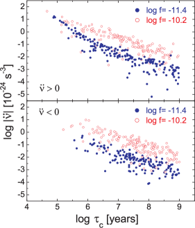
Figure 14: Simulations of the $|\ddot{\nu}|$-$\tau_{\rm c}$ distribution for $\alpha=0.5$, $T=30~{}{\rm yr}$. The results with parameter set $(-11.35,0.01)$ and $(-10.2,0.01)$ for $\log f$ are shown by unfilled circles and filled circles, respectively.

3.2.3 Effects of Oscillation Amplitude

We assume the oscillation amplitude parameter set for $\log f$ is $(\mu,\sigma)=(-11.35,0.01)$ and $(-10.2,0.01)$, respectively. The simulated results for $\alpha=0.5$ and $T=30~{}{\rm yr}$ are shown in Figure 14. One can obtain two conclusions from the figure: (a) a larger $\log f$ makes an upper distribution envelop higher (with larger $|\ddot{\nu}|$, as predicted by Equation (11), and (b) the lower distribution envelop shows a steeper slope for the segment of $\tau_{\rm c}\lesssim 10^{6}~{}{\rm yr}$ for $\ddot{\nu}>0$.

$N_{\rm p}\approx N_{\rm n}$ is an important constraint for the model. It is found that if $\log f\gtrsim-11.4$ (i.e. $k\gtrsim 6\times 10^{-4}$ for $T=30~{}{\rm yr}$), $N_{\rm p}\approx N_{\rm n}$ for the case of $\alpha=0.5$ (e.g. we perform a simulation with $(\mu=-10.3,\sigma=1)$ and $T=30~{}{\rm yr}$ and get $3494$ outcomes, in which $N_{\rm p}=1849$ and $N_{\rm p}/N_{\rm total}\simeq 52.9\%$); however, if $\log f\lesssim-11.4$, we will obtain $N_{\rm p}\gg N_{\rm n}$. The existence of the lower limit is mainly due to the competition between the magnetic field long-term decay and the short-term oscillation, as predicted by Equation (10). However, it is worth to note that the lower limit is larger than the analytical result $\log f\simeq-11.85$, as shown in Figure 9. This is caused by the “averaging” effect that induced an underestimation for $|\ddot{\nu}|$. Meanwhile, it is also found that $|\ddot{\nu}|$ will be larger than the $2\sigma$ range of the reported data if $\log f\gtrsim-10.2$ (i.e. $k\gtrsim 0.01$ for $T=30~{}{\rm yr}$). In conclusion, the upper and lower bounds of $\log f$ (for $\alpha=0.5$) can be obtained by using the conditions of $N_{\rm p}\approx N_{\rm n}$ and the upper boundary of reported data: $-11.4\lesssim\log f\lesssim-10.2$.

Based on the constraints for $T$ and $\log f$ and many similar simulations as described above, we find the best parameters are: $\alpha=0.5$, $T=30~{}{\rm yr}$ and $(\mu=-11.35,\sigma=1.0)$ for $\log f$. We show the simulated results with these parameters in Figure 15, in which $N_{\rm total}=3606$, $N_{\rm p}=1950$ and $N_{\rm n}=1681$. $N_{\rm p}/N_{\rm total}\approx 54\%$. For $\ddot{\nu}>0$ about $93.4\%$ and $69.4\%$ of the reported data are covered by the $2\sigma$ and $1\sigma$ areas of the simulated data, respectively; similarly, for $\ddot{\nu}<0$ about $90.0\%$ and $65.8\%$ of the reported data are covered by the $2\sigma$ and the $1\sigma$ areas, respectively. Though the slope ($b=-1.81$) for the young pulsars with $\tau_{\rm c}<10^{6}~{}{\rm yr}$ is still slightly too flat, the three slopes are generally consistent with slopes of reported data. Compared with the case of $T=20~{}{\rm yr}$, the $2\sigma$ area overlaps with the reported data points better.

In the bottom four panels of Figure 15, we compare the observed and simulated correlations between $\tau_{c}$ for $n>0$ (left panels) and $n<0$ (right panels), respectively; the general trends of the data are also reproduced. The linear fits for $\log|n|~{}[10^{-24}~{}{\rm s^{-3}}]=d+h\log\tau_{c}~{}[{\rm yr}]$ are given, and for both the observed data and simulated data, $h\simeq 1$. For $n>0$ about $84.2\%$ and $59.5\%$ of the reported data are covered by the $2\sigma$ and $1\sigma$ areas of the simulated data, respectively; similarly, for $n<0$ about $93.0\%$ and $56.9\%$ of the reported data are covered by the $2\sigma$ and the $1\sigma$ areas, respectively. However, one can see that the simulated $|n|$ are systematically larger than the reported results. This situation can be improved by setting a smaller $f$, which however will result in $N_{\rm p}\gg N_{\rm n}$.

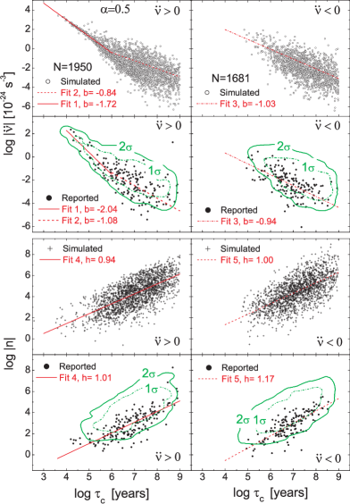
Figure 15: Simulations of the $|\ddot{\nu}|$-$\tau_{\rm c}$ distribution (upper panels) in the cases of moderate long term magnetic field decay ($\alpha=0.5$) and correlations of $n$ with $\tau_{c}$ (bottom panels). Linear fit 1: for $\ddot{\nu}>0$ with $\tau_{\rm c}<10^{6}~{}{\rm yr}$; Linear fit 2: for $\ddot{\nu}>0$ with $10^{6}~{}{\rm yr}<\tau_{\rm c}<10^{8}~{}{\rm yr}$; Linear fit 3: for $\ddot{\nu}<0$ with $\tau_{\rm c}<10^{8}~{}{\rm yr}$; Linear fit 4: for $n>0$; Linear fit 5: for $n<0$. The best-fit slopes ($b$ and $h$) for all simulations and reported data are labelled in these corresponding panels.

3.2.4 The Two-dimensional Kolmogorov-Smirnov Test

Here we perform the two-dimensional Kolmogorov-Smirnov (2DKS) test to reexamine the distributions of the simulated results using the KS2D package. Our purpose is to test the consistency of the distributions of reported data and the simulated data in Figure 11, and we show the returned probabilities in Table 2. If the returned probability is greater than 0.2, then it is a sign that you can treat them as drawn from the same distribution. One can see that the simulated results, for all values of $\alpha$, are apparently rejected by the test. However, some of the main features of the distributions can be reproduced by the model, as we discussed above. On the other hand, the 2DKS test indicates that $\alpha=0.5$ is still relatively better than the others.

The failures to the 2DKS tests mean that our model is too simple, and the discrepancy is mainly caused by the larger $|\ddot{\nu}|$ given by the model based on the sample space. The possible reasons are: (1) the magnetic field of old pulsars have no long-term decay; (2) the median value of the magnetic inclination angle is apparently smaller than $\pi/2$, i.e. $\theta\ll\pi/2$, since a smaller $\theta$ corresponds to a longer $t$, and thus a smaller $\ddot{\nu}$, as predicted by Equation (10); (3) we assume all the pulsars have the same $k$ and $T$, and with only one oscillation component; and (4) As argued in H2010, the timing noise in some young pulsars is dominated by “glitch recovery”, which cannot be modelled by the present model and thus should cause some discrepancies from our model predictions.

Table 2: The returned probabilities of 2DKS test for simulated data with reported data. If the probability is greater than 0.2, then them can be treated as drawn from the same distribution.

  Database $P(\ddot{\nu}>0)$ $P(\ddot{\nu}<0)$ $\alpha=0.0$ $9.63\times 10^{-9}$ $1.49\times 10^{-12}$ $\alpha=0.5$ $3.09\times 10^{-6}$ $3.14\times 10^{-9}$ $\alpha=1.0$ $1.29\times 10^{-7}$ $5.24\times 10^{-12}$  

4 Summary and Discussion

In this work we first modeled the $\ddot{\nu}$ and $n$ evolutions and applied the obtained model parameters to simulating the timing residuals for the individual pulsar PSR B0329+54. Using a Monte Carlo simulation method, we simulated the distributions of pulsars in the $|\ddot{\nu}|-\tau_{\rm c}$ and $|n|-\tau_{\rm c}$ diagrams, and compared the simulation results with the reported data in H2010. Our main results are summarized as follows:

1. We modeled the $\ddot{\nu}$ evolution of pulsar PSR B0329+54 with the phenomenological model of the evolution of $B$, which contains a long-term decay ($\alpha=0.5$) modulated by two short-term oscillations (upper panels of Figure 1). The model can reproduce the main characteristics of the $|\ddot{\nu}|$ variation, including the swings between $\ddot{\nu}>0$ and $\ddot{\nu}<0$.

2. For PSR B0329+54, besides a $16.8~{}{\rm yr}$ component as reported by Shabanova (1995), we find that the pulsar has an another oscillation component with period ($\sim 50~{}{\rm yr}$) longer than the current span of timing observations. This two component model predicts that another swing of the sign of $\ddot{\nu}>0$ has happened recently or in the very near future, which can be tested by analysing the recent observation data.

3. We showed that the “averaged” values of $n$ are different from the instantaneous values (bottom panels of Figure 1), and the oscillation abruptly decays after the first period due to the “averaging” effect. Using these parameters obtained from modeling the $\ddot{\nu}$ evolution, we simulated the timing residuals of the pulsar (Figure 3), which agrees with the reported residuals (H2010) well.

4. We performed Monte Carlo simulations for the distribution of $|\ddot{\nu}|$ in the $|\ddot{\nu}|-\tau_{\rm c}$ diagram. Our results for different modes of magnetic field long-term decay (i.e. $\alpha=0$, $0.5$ and $1.0$) are presented in Figures 11 and 12. It is found that the mode of $\alpha=0.5$ may dominate the magnetic field decay for young pulsars.

5. By overlapping the $2\sigma$ areas and comparing the distribution density and overall shape of simulated results with the reported data, we found that the oscillation period $30~{}{\rm yr}\lesssim T\lesssim 1000~{}{\rm yr}$.

6. The observed $N_{\rm p}\approx N_{\rm n}$ can be obtained if the oscillation parameter $\log f\gtrsim-11.4$, which is larger the analytical prediction of $\log f\thickapprox-11.85$ (Figure 9). This is due to the “averaging” effect not included in our previous analytical study. The upper limit for the oscillation parameter is $\log f\lesssim-10.2$, which is derived from the upper boundary of the $2\sigma$ area of reported data.

7. The distribution of $n$ is also presented with the $|\ddot{\nu}|-\tau_{\rm c}$ diagram in Figure 15, and the observed correlations are well reproduced. However the simulated envelop of $|n|$ are higher than the reported data.

In the model, there are no significant differences for the cases with oscillation period between thirty years to few hundred years in the simulations. However, it is pointed out that the “averaging” effect still has an influence on the parameters of oscillation amplitude, i.e. on the mean value of $\log f$. Thus, an average period about several decades years is preferred. Pons et al. (2012) proposed a similar model of magnetic field oscillations, obtained pulsar evolutionary tracks in $P-\dot{P}$ diagram, and explained the observed braking indices of older pulsars. In their model the magnetic field oscillations are identified as due to the Hall drift effect in the crust of neutron stars, with a timescale of $(10^{6}-10^{8})\frac{10^{12}~{}G}{B}~{}{\rm yr}$ and magnitude $\delta B/B\sim 10^{-3}$. They showed that a cubic pattern would dominate the timing residual, on the condition that the magnitude of a sinusoidal or a random perturbation is smaller than the magnitude of the oscillation.

We suggest that the Hall drift effect may play a role for older pulsars; however, it is probably not a dominant mechanism for most pulsars, since the corresponding oscillation periods are too long. Lyne et al. (2010) showed credible evidence that timing residuals and $\dot{\nu}$ are connected with changes in the pulse width. Therefore, timing residuals are more likely caused by the changes in a pulsar’s magnetosphere with periods about $1-100~{}{\rm yr}$. On the other hand, in the $|\ddot{\nu}|-\tau_{\rm c}$ diagram the clusters at the old age area ($\tau_{c}>10^{6}~{}{\rm yr}$) are due to the fact that the oscillation term dominates in low $|\dot{\nu}|$ pulsars, as we showed in Figure 12. Thus the oscillation period as long as $10^{6}~{}{\rm yr}$ is not necessary. Particularly for those pulsars like PSR B0329+54, $\ddot{\nu}$ switches between positive values and negative values and $\ddot{\nu}$ evolution and timing residuals are coupled. These observations cannot be understand by oscillations with period as long as million years. However, they can be well reproduced by the model that involves magnetic field oscillations with periods of $\sim 30-100~{}{\rm yr}$.

References

- (1) Alpar, M. A., Nandkumar, R., Pines, D. 1986, ApJ, 311, 197
- (2) Bailes, M., Lyne, A. G., & Shemar, S. L. 1993, ASPC,36,19B
- (3) Baykal, A., Ali Alpar, M., Boynton, P. E., & Deeter, J. E. 1999, MNRAS, 306, 207
- (4) Blandford, R. D., & Romani, R. W. 1988, MNRAS, 234, 57P
- (5) Boynton, P. E., et al. 1972, ApJ, 175, 217
- (6) Cheng, K. S. 1987, ApJ, 321, 799
- (7) Cheng, K. S. 1987, ApJ, 321, 805
- (8) Chukwude, A. E. 1975, 2003, A&A, 406,667
- (9) Coles, W., Hobbs, G., Champion, D. J., Manchester, R. N., & Verbiest, J. P. W. 2011, MNRAS, 418, 561
- (10) Cordes, J. M. 1980, ApJ, 237, 216
- (11) Cordes, J. M., & Downs, G. S. 1985, ApJS, 59, 343
- (12) Cordes, J. M. & Helfand, D. J. 1980, ApJ, 239, 640
- (13) Cordes, J. M., & Shannon, R. M. 2008, ApJ, 682,1152
- (14) D’Alessandro, F., McCulloch, P. M., Hamilton, P. A., & Deshpande, A. A. 1995, MNRAS, 277, 1033
- (15) Demiaski & Prszyski, 1979, Nature, 282, 383
- (16) Groth, E. J. 1975, ApJS, 29, 431
- (17) Gullahorn, G. E., & Rankin, J. M. 1978, AJ, 83,1219
- (18) Helfand, D. J., Taylor, J. H., Backus, P. R., & Cordes, J. M. 1980, ApJ, 237, 206
- (19) Hobbs, G., Lyne, A. G., & Kramer, M. 2010, MNRAS, 402, 1027
- (20) Jones, D. I. 2012, MNRAS, 420, 2325
- (21) Jones, P. B. 1982, MNRAS, 200, 1081
- (22) Kaspi, V. M., Chakrabarty, D., & Steinberger, J. 1999, ApJ, 525,33
- (23) Konacki, M., Lewandowski, W., Wolszczan, A., Doroshenko, O., & Kramer, M. 1999, ApJ, 519, L81
- (24) Liu, X. W., Na, X. S., Xu, R. X., & Qiao, G. J. 2011, Chin. Phys. Lett., 28, 019701
- (25) Livingstone, M. A., Kaspi, V. M., Gavriil, F. P., & Manchester, R. N. 2005, ApJ, 619, 1046
- (26) Lyne, A., Hobbs, G., Kramer, M., Stairs, I., & Stappers, B. 2010, Science, 329, 408
- (27) Manchester, R. N., & Taylor, J. H. 1977, in Pulsars, ed. R. N. Manchester & J. H. Taylor (San Francisco, CA: W. H. Freeman), 281
- (28) Pons, J. A., Vigan, D., & Geppert, U. 2012, A&A, 547, A9
- (29) Shabanova, T. V. 1995, ApJ, 453, 779
- (30) Shannon, R. M., & Cordes, J. M. 2010, ApJ, 725, 1607
- (31) Stairs, I. H., Lyne, A. G., & Shemar, S. L. Nature, 406, 484
- (32) Qiao, G. J., Xue, Y. Q., Xu, R. X., Wang, H. G., & Xiao, B. W. 2003, A&A, 407, L25
- (33) Zhang, S.-N., & Xie, Y. 2012, ApJ, 757, 153 (Paper I)
- (34) Zhang, S.-N., & Xie, Y. 2012, ApJ, 761, 102 (Paper II)