Elemental and tight monogamy relations in nonsignalling theories

Abstract

Physical principles constrain the way nonlocal correlations can be distributed among distant parties. These constraints are usually expressed by monogamy relations that bound the amount of Bell inequality violation observed among a set of parties by the violation observed by a different set of parties. We prove here that much stronger monogamy relations are possible for nonsignalling correlations by showing how nonlocal correlations among a set of parties limit any form of correlations, not necessarily nonlocal, shared among other parties. In particular, we provide tight bounds between the violation of a family of Bell inequalities among an arbitrary number of parties and the knowledge an external observer can gain about outcomes of any single measurement performed by the parties. Finally, we show how the obtained monogamy relations offer an improvement over the existing protocols for device-independent quantum key distribution and randomness amplification.

Introduction. It is a well established fact that entanglement and nonlocal correlations (cf. Refs. Hreview ; NLreview ), i.e., correlations violating a Bell inequality Bell , are fundamental resources of quantum information theory. It has been confirmed by many instances that, when distributed among spatially separated observers, they give an advantage over classical correlations at certain information-theoretic tasks, many of them being considered in the multipartite scenario. For instance, nonlocal correlations outperform their classical counterpart at communication complexity problems CommCompl , and allow for security not achievable within classical theory crypto .

Physical principles impose certain constraints on the way these resources can be distributed among separated parties; these are commonly referred to as monogamy relations. For instance, in any three–qubit pure state one party cannot share large amount of entanglement, as measured by concurrence, simultaneously with both remaining parties Wootters . Analogous monogamy relations, both in qualitative NS ; BarrettMon ; BKP ; rodrigo and quantitative TV ; T form, were demonstrated for nonlocal correlations, with the measure of nonlocality being the violation of specific Bell inequalities. In particular, Toner and Verstraete TV and later Toner T showed that if three parties $A$, $B$, and $C$ share, respectively, quantum and general nonsignalling correlations, then only a single pair can violate the Clauser-Horne-Shimony-Holt (CHSH) Bell inequality CHSH . These findings were generalized to more complex scenarios ns-mon ; Pawel (see also Ref. Thiago ), and in particular in ns-mon a general construction of monogamy relations for nonsignalling correlations from any bipartite Bell inequality was proposed.

In this work, we demonstrate that nonsignalling correlations are monogamous in a much stronger sense: the amount of nonlocality observed by a set of parties may imply severe limitations on any form of correlations with other parties. That is, instead of comparing nonlocality between distinct groups of parties, we rather relate it to the knowledge that external parties can gain on outcomes of any of the measurements performed by the parties (see Fig. 1). To be more illustrative, consider again parties $A$, $B$, and $C$ performing a Bell experiment with $M$ observables and $d$ outcomes. We construct tight bounds between the violation of certain Bell inequalities BKP among any pair of parties, say $A$ and $B$, and classical correlations that the third party $C$ can establish with outcomes of any measurement performed by $A$ or $B$. This means that the amount of any correlations — classical or nonlocal — that $C$ could share with $A$ or $B$ is bounded by the strength of the Bell inequality violation between $A$ and $B$. Our monogamies are further generalized to the scenario with an arbitrary number of parties $N$ [$(N,M,d)$ scenario] with nonlocality measured by the recent generalization of the Bell inequalities BKP presented in Ref. rodrigo . The obtained monogamy relations are logically independent from, and in fact stronger than, the existing relations involving only nonlocal correlations, as a bound on nonlocal correlations does not necessarily imply any nontrivial constraint on the amount of classical correlations.

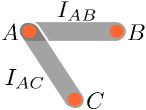
(a) (b)

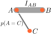
Figure 1: (a) The usual monogamies compare nonlocality (measured by the value of some Bell inequality $I$) between different groups of parties (here between two pairs of parties $AB$ and $AC$). Instead, our monogamy relations compare nonlocality observed by a group of parties (here $AB$) to the knowledge, represented by the probability $p(A=C)$, that the third party $C$ can have about outcomes observed by either of the parties. As such, they are qualitatively different, and in fact stronger than those of type (a).

Our new monogamy relations prove useful in device-independent protocols device-ind ; DIRNG ; collbeck-renner ; andrzej ; qit . First, we show that they impose tight bounds on the guessing probability, the commonly used measure of randomness, that are significantly better than the existing ones BKP ; rodrigo . We then argue that this translates into superior performance in protocols for device-independent quantum key distribution (DIQKD) Lluis2 using measurements with more than two outputs. Finally, we show that they allow for a generalization of the results of collbeck-renner on randomness amplification to any number of parties and outcomes, demonstrating, in particular, that arbitrary amount of arbitrarily good randomness can be amplified in a bipartite setup.

Before turning to the results, we provide some background. Consider $N$ parties $A^{(1)},\ldots,A^{(N)}$ (for $N=3$ denoted by $A,B,C$), each measuring one of $M$ possible observables $A^{(i)}_{x_{i}}$ $(x_{i}=1,\ldots,M)$ with $d$ outcomes (enumerated by $a_{i}=1,\ldots,d$) on their local physical systems. The produced correlations are described by a collection of probabilities $p(A^{(1)}_{x_{1}}=a_{1},\ldots,A^{(N)}_{x_{N}}=a_{N})\equiv p(a_{1}\ldots a_{N}|x_{1}\ldots x_{N})\equiv p(\boldsymbol{a}|\boldsymbol{x})$ of obtaining results $\boldsymbol{a}\equiv a_{1}\ldots a_{N}$ upon measuring $\boldsymbol{x}\equiv x_{1}\ldots x_{N}$. One then says that the correlations $\{p(\boldsymbol{a}|\boldsymbol{x})\}$ are (i) nonsignalling (NC) if any of the marginals describing a subset of parties is independent of the measurements choices made by the remaining parties and (ii) quantum (QC) if they arise by local measurements on quantum states (cf. NLreview ).

Elemental and tight monogamies for nonsignalling correlations. We start with the derivation of our monogamy relations in the case of nonsignalling correlations. For clarity, we begin with the simplest tripartite scenario. We will use the Bell inequality introduced by Barrett, Kent, and Pironio (BKP) BKP . Denoting by $\langle\Omega\rangle$ the mean value of a random variable $\Omega$, that is, $\langle\Omega\rangle=\sum_{i=1}^{d-1}iP(\Omega=i)$, it reads

$$I^{2,M,d}_{AB}:=\sum_{\alpha=1}^{M}\left(\langle[A_{\alpha}-B_{\alpha}]\rangle+\langle[B_{\alpha}-A_{\alpha+1}]\rangle\right)\geq d-1$$ (1)

with $[\Omega]$ being $\Omega$ modulo $d$, and $\Omega_{M+1}:=[\Omega_{1}+1]$. For $d=2$, Ineq. (1) reproduces the chained Bell inequalities BC , while for $M=2$ the Collins-Gisin-Linden-Massar-Popescu (CGLMP) inequalities Collins . The maximal nonsignalling violation of (1) is $I_{AB}^{2,M,d}=0$.

The only monogamy relations for (1) have been formulated in terms of its violations between Alice and $M$ Bobs ns-mon , which is a natural quantitative extension of the concept of $M$-shareability NS . In the following theorem we show that the BKP Bell inequalities allow one to introduce elemental monogamies obeyed by any NC.

Theorem 1.

For any tripartite NC $\{p(abc|xyz)\}$ with $M$ $d$-outcome measurements, the inequality

$$I^{2,M,d}_{AB}+\langle[X_{i}-C_{j}]\rangle+\langle[C_{j}-X_{i}]\rangle\geq d-1$$ (2)

holds for any pair $i,j=1,\ldots,M$ and $X$ denoting $A$ or $B$.

Interestingly, all these inequalities are tight in the sense that for any values of $I_{AB}^{2,M,d}$ and $\langle[X_{i}-C_{j}]\rangle+\langle[C_{j}-X_{i}]\rangle$ saturating (2), one can find NC realizing these values. Take, for instance, a probability distribution $\{p(a,b,c|x,y,z)=p(a,b|x,y)p(c|z)\}$, with $\{p(a,b|x,y)\}$ being a mixture of a nonlocal model maximally violating (1) and a local deterministic one saturating it. Then, $\{p(c|z)\}$ is the same distribution as the one used by $A$ or $B$ in the local model saturating (1).

The physical interpretation of our monogamies can be now concluded if we rewrite them in a bit different form. Using the fact that for any variable $\Omega$, $\langle[\Omega]\rangle+\langle[-\Omega]\rangle=dP([\Omega]\neq 0)=d[1-P([\Omega]=0)]$ supplement , Ineqs. (2) transform to

$$I^{2,M,d}_{AB}+1\geq dp(X_{i}=C_{j})$$ (3)

for $X=A,B$, and any pair $i,j=1,\ldots,M$. These relations hold if $AB$ is replaced by any pair of parties and if any $m=1,\ldots,d-1$ is added modulo $d$ to the argument of probability. The meaning of the introduced monogamy relations is now transparent. The probability $p(X_{i}=C_{j})$ that parties $X$ and $C$ obtain the same results upon measuring the $i$th and $j$th observables is a measure of how the outcomes of these measurements are classically correlated. Consequently, Ineqs. (2) establish trade-offs between nonlocality, as measured by (1), that can be generated between any two parties and classical correlations that the third party can share with the results of any measurement performed by any of these two parties. Furthermore, they are tight. In fact, it is known that the maximal NC violation of (1), $I^{2,M,d}_{AB}=0$, implies $p(X_{i}=C_{j})=1/d$ for any $i,j=1,\ldots,M$, meaning that at the point of maximal violation $C$ cannot share any correlations with any other party’s measurement outcomes BKP . On the other hand, it is well known that at the point of no violation $C$ can be arbitrarily correlated with $A$ and $B$. For intermediate violations, the best one can hope for is a linear interpolation between these two extreme values and this is precisely what our monogamy relations predict, see Fig. 2.

Let us now move to the general case of an arbitrary number of parties each having $M$ $d$-outcome observables at their disposal. We will utilize the generalization of the Bell inequality (1) introduced in Ref. rodrigo , which can be stated as

$$I_{\mathsf{A}}^{N,M,d}\geq d-1$$ (4)

with $\mathsf{A}=A^{(1)}\ldots A^{(N)}$. Since the form of $I_{\mathsf{A}}^{N,M,d}$ is rather lengthy and actually not relevant for further considerations, for clarity, we omit presenting it here (see supplement ). We only mention that it can be recursively determined from $I_{AB}^{2,M,d}$ and that its minimal nonsignalling value is $I_{\mathsf{A}}^{N,M,d}=0$. Then, the generalization of Theorem 1 to arbitrary $N$ goes as follows.

Theorem 2.

For any $(N+1)$–partite NC $\{p(\boldsymbol{a}|\boldsymbol{x})\}$ with $M$ $d$-outcome measurements per site, the following inequality

$$I^{N,M,d}_{\mathsf{A}}+\langle[A_{x_{k}}^{(k)}-A^{(N+1)}_{x_{N+1}}]\rangle+\langle[A^{(N+1)}_{x_{N+1}}-A_{x_{k}}^{(k)}]\rangle\geq d-1$$ (5)

is satisfied for any $x_{k},x_{N+1}=1,\ldots,M$ and $k=1,\ldots,N$.

All the properties of the three-partite monogamy relations persist for any $N$. In particular, all inequalities (5) are tight. Moreover, they can be rewritten as

$$I^{N,M,d}_{\mathsf{A}}+1\geq dp(A^{(k)}_{x_{k}}=[A^{(N+1)}_{x_{N+1}}+m])$$ (6)

for any $x_{k},x_{N+1}=1,\ldots,M$, $k=1,\ldots,N$ and $m=0,\ldots,d-1$ and remain valid if the nonlocality is tested among any $N$-element subset of $N+1$ parties. Analogously to the three-partite case, Ineqs. (6) tightly relate the nonlocality observed by any $N$ parties, as measured by $I_{\mathsf{A}}^{N,M,d}$, and correlations that party $(N+1)$ can share between measurement outcomes of any of these $N$ parties. It is worth pointing out that for $d=2$ it holds $\langle[X-Y]\rangle=\langle[Y-X]\rangle$, and Ineqs. (5) simplify to $I^{N,M,2}_{\mathsf{A}}+2\langle[A_{x_{k}}^{(k)}-A^{(N+1)}_{x_{N+1}}]\rangle\geq 1$ which can be rewritten in a more familiar form as $|\langle A_{x_{k}}^{(k)}A^{(N+1)}_{x_{N+1}}\rangle|\leq I^{N,M,2}_{\mathsf{A}}$, where $A_{x_{k}}^{(k)}$ stand now for dichotomic observables with outcomes $\pm 1$, while $\langle XY\rangle=P(X=Y)-P(X\neq Y)$. Thus, the strength of violation of (24) imposes tight bounds on a single mean value $\langle A_{x_{k}}^{(k)}A^{(N+1)}_{x_{N+1}}\rangle$ for any $x_{k},x_{N+1}$ and $k=1,\ldots,N$, which is also a measure of how outcomes of a measurement performed by the external party $A^{(N+1)}$ are correlated to those of $A^{(k)}$ for any $k$. In particular, when $I_{\mathsf{A}}^{N,M,2}=0$ (maximal nonsignalling violation), all these means are zero, while maximal correlations between a single pair of measurements, i.e., $\langle A^{(k)}_{x_{k}}A^{(N+1)}_{x_{N+1}}\rangle=\pm 1$ for some $x_{k},x_{N+1}$, make the $N$ parties unable to violate $I_{\mathsf{A}}^{N,M,2}\geq 1$.

Bounds on randomness. Our monogamies are of particular importance for device–independent applications since they imply upper bounds on the guessing probability (GP) of the outcomes of any measurement performed by any of the $N$ parties by the additional party, here called $E$. To be precise, assume that $E$ has full knowledge about all parties devices and their measurement choices and wishes to guess the outcomes of, say $A_{x_{k}}^{(k)}$. The best $E$ can do for this purpose is to simply measure one of its observables, say the $z$th one, and, irrespectively of the obtained result, deliver the most probable outcome of $A^{(k)}_{x_{k}}$. Then, $\max_{a_{k}}p(A_{x_{k}}^{(k)}=a_{k})=p(E_{z}=A^{(k)}_{x_{k}})$, and Ineqs. (6) imply that for any $x_{k}$ and $k$, GP is bounded as

$$\max_{a_{k}}p(a_{k}|x_{k})\equiv\max_{a_{k}}p(A_{x_{k}}^{(k)}=a_{k})\leq\frac{1}{d}(1+I_{\mathsf{A}}^{N,M,d}).$$ (7)

These bounds are tight and significantly stronger than the previously existing one,

$$\max_{a_{k}}p(a_{k}|x_{k})\leq\frac{1}{d}\left(1+\frac{d^{N}}{4}(N-1)I_{\mathsf{A}}^{N,M,d}\right)$$ (8)

derived in Refs. BKP ; rodrigo (see Fig. 2).

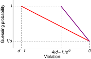
(a) (b)

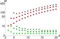
Figure 2: (a) Comparison of the upper bounds on GP: present bound (7) (red line) and (8) (purple line). Our bound is tight – for any value $0\leq I_{\mathsf{A}}^{N,M,d}\leq d-1$, it provides the maximum attainable value of GP. Instead, the bound (8) is nontrivial only in some restricted range of $I_{\mathsf{A}}^{N,M,d}$, namely when $I_{\mathsf{A}}^{N,M,d}<4(d-1)/d^{2}$, which tends to zero for $d\to\infty$. (b) Minimal number of measurements $M$ on a maximally entangled state of local dimension $d$ necessary for the secret-key rate $R$ secure against non-signalling eavesdroppers to be at least: one (dots), $\log_{2}3$ (squares), and two (triangles) bits, when (7) (green) and (8) (red) are used to bound $R$. Using our bound the parties need to use many fewer measurements to reach the same key rate. Moreover, contrary to what is predicted by the previous bound, the number of measurement decreases with the dimension.

Let us now discuss how the bound (7) performs in comparison to (8) in security proofs of DIQKD against no-signalling eavesdroppers. At the moment, a general security proof in this scenario is missing and the strongest proof requires the assumption that the eavesdropper $E$ is not only limited by the no-signalling principle but also lacks a long-term quantum memory (so–called bounded-storage model) Lluis2 . Assume that Alice and Bob share a two-qudit maximally entangled state and they use it to maximally violate (1) by performing the optimal measurements for this setup (see, e.g., BKP ). To generate the secure key, Bob performs one more measurement that is perfectly correlated to one of Alice’s measurements. The key rate of this protocol is lower-bounded as $R\geq-\log_{2}[\tau(I_{AB}^{2,M,d})]-H(A|B)$ Lluis2 , where $\tau$ is any upper bound on GP for nonsignalling correlations. and $H(A|B)$ is the conditional Shannon entropy between Alice and Bob for the measurements used to generate the secret key. As the state is maximally entangled, this term is equal to zero. Fig. 2 compares bounds on the secret key obtained by using our bound (7) and the previous bound (8) in this protocol. We fix the key rate and compute the minimal number of measurements needed to attain this rate using these bounds as a function of the number of outputs. As shown in Fig. 2, the number of measurements when using our bound is much smaller and, in particular, decreases with the number of outputs.

Randomness amplification. Let us finally show the usefulness of our monogamy relations in randomness amplification. Assume that each party is given a sequence of bits produced by the Santha–Vazirani (SV) source (or the $\varepsilon$–source). Its working is defined as follows: it produces a sequence $y_{1},y_{2},\cdots,y_{n}$ of bits according to

$$\tfrac{1}{2}-\varepsilon\leq p(y_{k}|w)\leq\tfrac{1}{2}+\varepsilon,\quad k=1,\ldots,n,$$ (9)

where $w$ denotes any space-time variable that could be the cause of $y_{k}$. Thus the bits are possibly correlated with each other retaining, however, some intrinsic randomness — we say that they are $\varepsilon$–free. The goal is now to obtain a perfectly random bit (or more generally $d$it) from an arbitrarily long sequence of $\varepsilon$–free bits by using quantum correlations that violate the Bell inequality (24). This procedure is called randomness amplification (RA).

It is useful to recast this task in the adversarial picture collbeck-renner , in which one assumes that an adversary $E$, using the $\varepsilon$–sources, wants to simulate the quantum violation of (24) by NC, in particular the local ones. The random variable $W$ is now held by $E$ who uses it to control both the $\varepsilon$-sources and the physical devices possessed by the parties. That is, for every value $w$ of $W$ the former provides settings $\boldsymbol{x}$ with probabilities obeying (45), while these devices generate the $N$-partite probability distribution $\{p(\boldsymbol{a}|\boldsymbol{x},w)\}_{\boldsymbol{a},\boldsymbol{x}}$. Using (7), we can now restate and generalize Lemma 1 of collbeck-renner (see supplement ).

Theorem 3.

Let $\{p(\boldsymbol{a}|\boldsymbol{x},w)\}_{\boldsymbol{a},\boldsymbol{x}}$ be a nonsignalling probability distribution for any $w$. Then for any $\boldsymbol{x}$ and $k=1,\ldots,N$:

$$\sum_{a_{k},w}\left|p(a_{k},w|\boldsymbol{x})-\widetilde{p}(a_{k})p(w|\boldsymbol{x})\right|\leq\tfrac{(d-1)^{2}+1}{d}\,Q_{M}(\boldsymbol{x})I^{N,M,d}_{\mathsf{A}},$$ (10)

where $\widetilde{p}(a)=1/d$ for any $a$, $\{p(a_{k},w|\boldsymbol{x})\}_{a_{k},w}$ describes correlations between outcomes obtained by party $k$ and the random variable $W$ for the measurements choice $\boldsymbol{x}$, and $I^{N,M,d}_{\mathsf{A}}$ is taken in the probability distribution $\{p(\boldsymbol{a}|\boldsymbol{x})\}$ observed by the parties. Finally, $Q_{M}(\boldsymbol{x})=\max_{w}[p(w|\boldsymbol{x})/p_{\min}(w)]$, where $p_{\min}(w)=\min_{\boldsymbol{x}}\{p(w|\boldsymbol{x})\}$ with minimum taken over those measurement settings $\boldsymbol{x}$ that appear in $I_{\mathsf{A}}^{N,M,d}$.

It then follows that if correlations $\{p(\boldsymbol{a}|\boldsymbol{x})\}$ violate maximally the Bell inequality (24), then the dits observed by the parties are perfectly random and uncorrelated from $W$ collbeck-renner .

Let us now show that one can amplify partially random input bits to almost perfectly random dits by using QC that produce arbitrarily high violation of $I_{\mathsf{A}}^{N,M,d}$. To generate one of the $M$ measurement settings, each party uses its SV source $r=\lceil\log_{2}M\rceil$ times. Hence for any $\boldsymbol{x}$, $Q_{r}(\boldsymbol{x})\leq[(1+2\varepsilon)/(1-2\varepsilon)]^{Nr}$ (cf. Ref. collbeck-renner ). Then, there is a state and measurement settings BKP ; rodrigo such that for large $M$,

$$I^{N,M,d}_{\mathsf{A}}\approx\lambda(d)/M\leq\lambda(d)/2^{r-1},$$ (11)

where $\lambda(d)$ is a function of $d$. After plugging everything into (10), one checks that its r.h.s. tends to zero for $M\to\infty$ iff $\varepsilon<\varepsilon_{N}:=(2^{1/N}-1)/[2(2^{1/N}+1)]$. As a result, QC violating (11) can be used to amplify randomness of any $\varepsilon$-source provided $\varepsilon<\varepsilon_{N}$. In particular, for $N=2$, the above reproduces the value $\varepsilon_{2}=(\sqrt{2}-1)^{2}/2$ found in collbeck-renner , and, because $\varepsilon_{N}$ is a strictly decreasing function of $N$, the larger $N$, the lower the critical epsilon $\varepsilon_{N}$ for this method to work. Notice, however, that $\varepsilon_{N}$ is independent of $d$, so almost perfectly random dits are obtained from partially random bits. This means that using the setup from Ref. collbeck-renner we can in fact achieve both amplification and expansion of randomness simultaneously.

Recently, with the same Bell inequality but for $N=d=2$, the critical epsilon was shifted from $\varepsilon_{2}\approx 0.086$ to $\varepsilon_{2}^{\prime}\approx 0.0961$ andrzej . We will now show that by using a slightly different approach the critical epsilon can be almost doubled. To this end, we exploit the fact that only $2M^{N-1}$ measurement settings out of all possible $M^{N}$ appear in $I_{\mathsf{A}}^{N,M,d}$. However, to generate them a common source has to be used. Assuming then that this is the case, $R=\log_{2}(2M^{N-1})=1+(N-1)r$ (instead of $Nr$) uses of the SV source are enough to generate all measurement settings in $I_{\mathsf{A}}^{N,M,d}$. Thus, $Q_{r}(\boldsymbol{x})\leq[(1+2\varepsilon)/(1-2\varepsilon)]^{1+(N-1)r}$, which together with (11) imply that the right-hand side of (10) vanishes for $M\to\infty$ iff $\varepsilon<\varepsilon_{N}^{\prime\prime}=(2^{1/(N-1)}-1)/[2(2^{1/(N-1)}+1)]$, and in particular $\varepsilon^{\prime\prime}_{2}=1/6>\varepsilon_{2}^{\prime}$.

Conclusions. We have presented a novel class of monogamy relations, obeyed by any nonsignalling physical theory. They tightly relate the amount of nonlocality, as quantified by the violation of Bell inequalities BKP ; rodrigo , that $N$ parties have generated in an experiment to the classical correlations an external party can share with outcomes of any measurement performed by the parties. Such trade–offs find natural applications in device-independent protocols and here we have discussed how they apply in quantum key distribution (cf. also Ref. 2prot ) and generation and amplification of randomness. We have finally showed that bipartite quantum correlations allow one to amplify $\varepsilon$–free $d$its for any $\varepsilon<1/6$.

Our results provoke further questions. First, it is natural to ask if analogous monogamies hold for quantum correlations, and, in fact, such elemental monogamies can be derived in the simplest (3,2,2) scenario (see supplement ). From a more fundamental perspective, it is of interest to understand what is the (minimal) set of of monogamy relations generating the same set of multipartite correlations as the no-signalling principle.

Acknowledgments. Discussions with Gonzalo De La Torre are gratefully acknowledged. This work is supported by NCN grant 2013/08/M/ST2/00626, FNP TEAM, EU project SIQS, ERC grants QITBOX, QOLAPS and QUAGATUA, the Spanish project Chist-Era DIQIP. This publication was made possible through the support of a grant from the John Templeton Foundation. R. A. also acknowledges the Spanish MINECO for the support through the Juan de la Cierva program.

I appendices

Here we present detailed proofs of Theorems 1, 2, and 3 of the main text. Also, in the simplest $(3,2,2)$ scenario we provide elemental monogamies for quantum correlations.

II Appendix A: Monogamy relations

II.1 Monogamy relations for nonsignalling correlations

Let us start with a simple fact. Recall for this purpose that $\langle\Omega\rangle$ is the standard mean value of a random variable $\Omega$, that is, $\langle\Omega\rangle=\sum_{i=1}^{d-1}iP(\Omega=i)$ and $[\Omega]$ stands for $\Omega$ modulo $d$.

Fact 1.

It holds that for any random variable $\Omega$,

$$(a) \hskip 28.45274pt\langle[\Omega]\rangle+\langle[-\Omega-1]\rangle=d-1,$$ (12)

$$(b) \hskip 28.45274pt\langle[\Omega]\rangle+\langle[-\Omega]\rangle=d[1-p([\Omega]=0)].$$ (13)

Proof.

Both equations follow from the very definition of $\langle[\cdot]\rangle$. To prove (a) we notice that $[-\Omega-1]+[\Omega]=d-1$, and hence

$$\langle[-\Omega-1]\rangle \negmedspace=\negmedspace \sum_{i=1}^{d-1}ip([\Omega]=d-i-1)$$ (14)

$$\negmedspace=\negmedspace \sum_{i=0}^{d-2}(d-i-1)p([\Omega]=i)$$

$$\negmedspace=\negmedspace (d-1)\sum_{i=0}^{d-2}p([\Omega]=i)-\sum_{i=0}^{d-2}iP([\Omega]=i)$$

$$\negmedspace=\negmedspace (d-1)\sum_{i=0}^{d-1}p([\Omega]=i)-\langle[\Omega]\rangle$$

$$\negmedspace=\negmedspace (d-1)-\langle[\Omega]\rangle,$$

where the second equality is a consequence of changing of the summation index, the fourth one stems from the definition of $\langle[\Omega]\rangle$ and rearranging terms, and the last equality follows from normalization.

To prove (b), we write

$$\langle[\Omega]\rangle+\langle[-\Omega]\rangle = \sum_{i=1}^{d-1}i[p([\Omega]=i)+p([-\Omega]=i)]$$ (15)

$$= \sum_{i=1}^{d-1}i[p([\Omega]=i)+p([\Omega]=d-i)]$$

$$= \sum_{i=1}^{d-1}ip([\Omega]=i)+\sum_{i=1}^{d-1}(d-i)p([\Omega]=i)$$

$$= d\sum_{i=1}^{d-1}p([\Omega]=i)$$

$$= d[1-p([\Omega]=0)],$$

where the second equality is a consequence of the fact that $[\Omega]+[-\Omega]=d$, while the third equality follows from shifting of the summation index in the second sum. ∎

Let us now move to the proofs of the monogamy relations. In the tripartite case we make use of the Barrett, Kent, and Pironio (BKP) BKP inequality

$$I^{2,M,d}_{AB}=\sum_{\alpha=1}^{M}\left(\langle[A_{\alpha}-B_{\alpha}]\rangle+\langle[B_{\alpha}-A_{\alpha+1}]\rangle\right)\geq d-1,$$ (16)

where the convention that $X_{M+1}=[X_{1}+1]$ is assumed.

Theorem 1.

For any three-partite nonsignalling correlations $\{p(a,b,c|x,y,z)\}$ with $M$ measurements and $d$ outcomes per site and any pair $\{i,j\}$ $(i,j=1,\ldots,M)$, the following inequality

$$I^{2,M,d}_{AB}+\langle[X_{i}-C_{j}]\rangle+\langle[C_{j}-X_{i}]\rangle\geq d-1$$ (17)

is satisfied with $X$ denoting either $A$ or $B$.

Proof.

Let us start with the case of $X=A$ and then notice that for a random variable $\Omega$ it holds that $\langle[\Omega]\rangle+\langle[-\Omega-1]\rangle=d-1$ (see Fact 1). Consequently,

$$\sum_{\begin{subarray}{c}\beta=1\\ \beta\neq i\end{subarray}}^{M}(\langle[C_{j}-A_{\beta}-1]\rangle+\langle[A_{\beta}-C_{j}]\rangle)-(M-1)(d-1)$$ (18)

is equal to zero. The fact that for any $\beta$ and $j$ it holds that $\langle[C_{j}-A_{\beta}-1]\rangle+\langle[A_{\beta}-C_{j}]\rangle=d-1=\langle[A_{\beta}-C_{j}-1]\rangle+\langle[C_{j}-A_{\beta}]\rangle$ allows us to rewrite (18) in the following way

$$\sum_{\beta=1}^{i-1}(\langle[C_{j}-A_{\beta}-1]\rangle+\langle[A_{\beta+1}-C_{j}]\rangle)$$

$$+\sum_{\beta=i+1}^{M}(\langle[A_{\beta}-C_{j}-1]\rangle+\langle[C_{j}-A_{\beta}]\rangle)-(M-1)(d-1).$$

Then, by adding $\langle[A_{i}-C_{j}]\rangle+\langle[C_{j}-A_{i}]\rangle$ to both sides of the above and rearranging some terms in the resulting expression, one obtains

$$\langle[A_{i}-C_{j}]\rangle+\langle[C_{j}-A_{i}]\rangle$$

$$=\sum_{\beta=1}^{i-1}(\langle[C_{j}-A_{\beta}-1]\rangle+\langle[A_{\beta+1}-C_{j}]\rangle)$$

$$+\sum_{\beta=i}^{M-1}(\langle[A_{\beta+1}-C_{j}-1]\rangle+\langle[C_{j}-A_{\beta}]\rangle)$$

$$+\langle[A_{1}-C_{j}]\rangle+\langle[C_{j}-A_{M}]\rangle-(M-1)(d-1).$$ (20)

In an analogous way, we may decompose $I_{AB}^{2,M,d}$:

$$I_{AB}^{2,M,d} = \sum_{\alpha=1}^{i-1}(\langle[A_{\alpha}-B_{\alpha}]\rangle+\langle[B_{\alpha}-A_{\alpha+1}]\rangle)$$ (21)

$$+\sum_{\alpha=i}^{M-1}(\langle[A_{\alpha}-B_{\alpha}]\rangle+\langle[B_{\alpha}-A_{\alpha+1}]\rangle)$$

$$+\langle[A_{M}-B_{M}]\rangle+\langle[B_{M}-A_{1}-1]\rangle.$$

In the last step of these manipulations, we add line by line Eqs. (II.1) and (21) in order to finally obtain

$$I_{AB}^{2,M,d}+\langle[A_{i}-C_{j}]\rangle+\langle[C_{j}-A_{i}]\rangle = \sum_{\alpha=1}^{i-1}(\langle[C_{j}-A_{\alpha}-1]\rangle+\langle[A_{\alpha}-B_{\alpha}]\rangle+\langle[B_{\alpha}-A_{\alpha+1}]\rangle+\langle[A_{\alpha+1}-C_{j}]\rangle)$$ (22)

$$+\sum_{\alpha=i}^{M-1}(\langle[C_{j}-A_{\alpha}]\rangle+\langle[A_{\alpha}-B_{\alpha}]\rangle+\langle[B_{\alpha}-A_{\alpha+1}]\rangle+\langle[A_{\alpha+1}-C_{j}-1]\rangle)$$

$$+\langle[C_{j}-A_{M}]\rangle+\langle[A_{M}-B_{M}]\rangle+\langle[B_{M}-A_{1}-1]\rangle+\langle[A_{1}-C_{j}]\rangle$$

$$-(M-1)(d-1).$$

What we have arrived at is basically the sum of $M$ Bell expressions $I^{2,2,d}$ but ‘distributed’ among three parties in such a way that Bob and Charlie measure only a single observable. It was shown in ns-mon that the minimal value such an expression can achieve over nonsignalling correlations is precisely its classical bound $d-1$. As a result, $I^{2,M,d}_{AB}+\langle[A_{i}-C_{j}]\rangle+\langle[C_{j}-A_{i}]\rangle\geq M(d-1)-(M-1)(d-1)=d-1$, finishing the proof for the case $X=A$.

If $X=B$ in Ineq. (17), then it suffices to rewrite the Bell expression from (16) as

$$I^{2,M,d}_{AB}=\sum_{\alpha=1}^{M}(\langle[B_{\alpha}-A_{\alpha+1}]\rangle+\langle[A_{\alpha+1}-B_{\alpha+1}]\rangle),$$ (23)

add to it the zero expression (18) with $A$ replaced by $B$, and repeat the above manipulations. This completes the proof. ∎

Now let us move to the general $(N,M,d)$ scenario. The inequality of interest is now the one from Ref. rodrigo , namely:

$$I^{N,M,d}_{\mathsf{A}}=\frac{1}{M}\sum_{\alpha_{N-1}=1}^{M}I_{A^{(1)}\ldots A^{(N-1)}}^{N-1,M,d}(\alpha_{N-1})\circ A^{(N)}_{\alpha_{N-1}}$$ (24)

$$\geq d-1.$$

where $\mathsf{A}=A^{(1)}\ldots A^{(N)}$. The notation $\circ A^{(i)}_{\gamma}$ means insertion of $A^{(i)}_{\gamma}$ to the average $\langle\cdot\rangle$ with the opposite sign to the one of $A^{(i-1)}_{\delta}$ with any $\gamma,\delta$, while $I_{A^{(1)}\ldots A^{(N-1)}}^{N-1,M,d}(\alpha_{N-1})$ is the same Bell expression as in (24), but for $N-1$ parties, and with observables of the last party relabeled as $\alpha_{N-2}\to\alpha_{N-2}+\alpha_{N-1}-1$ with $\alpha_{N}=1,\ldots,M$.

Theorem 2.

For any $(N+1)$-partite nonsignalling correlations $\{p(\boldsymbol{a}|\boldsymbol{x})\}$ with $M$ $d$-outcome measurements per site, the following inequality

$$I^{N,M,d}_{\mathsf{A}}+\langle[A_{x_{k}}^{(k)}-A^{(N+1)}_{x_{N+1}}]\rangle+\langle[A^{(N+1)}_{x_{N+1}}-A_{x_{k}}^{(k)}]\rangle\geq d-1$$ (25)

is satisfied for any $x_{k},x_{N+1}=1,\ldots,M$ and $k=1,\ldots,N$.

Proof.

The recursive formula in Ineq. (24), which for convenience we restate here

$$I^{N,M,d}_{\mathsf{A}}=\frac{1}{M}\sum_{\alpha_{N-1}=1}^{M}I_{A^{(1)}\ldots A^{(N-1)}}^{N-1,M,d}(\alpha_{N-1})\circ A^{(N)}_{\alpha_{N-1}},$$ (26)

allows us to demonstrate the theorem inductively. The case of $N=2$ has already been proved as Theorem 1, so we consider $N=3$. Exploiting Eq. (26), one can express $I^{3,M,d}_{A^{(1)}A^{(2)}A^{(3)}}$ as

$$I^{3,M,d}_{A^{(1)}A^{(2)}A^{(3)}}=\frac{1}{M}\sum_{\alpha_{2}=1}^{M}I^{2,M,d}_{A^{(1)}A^{(2)}}(\alpha_{2})\circ A^{(3)}_{\alpha_{2}}.$$ (27)

It is clear that for every $\alpha_{2}=1,\ldots,M$

$$I^{2,M,d}_{A^{(1)}A^{(2)}}(\alpha_{2}) = \sum_{\alpha_{1}=1}^{M}(\langle[A^{(1)}_{\alpha_{1}}-A^{(2)}_{\alpha_{1}+\alpha_{2}-1}]\rangle$$

$$\hskip 28.45274pt+\langle[A^{(2)}_{\alpha_{1}+\alpha_{2}-1}-A^{(1)}_{\alpha_{1}+1}]\rangle)\geq d-1$$

is a Bell inequality equivalent to (16), in which the observables of the second party $A^{(2)}$ have been relabelled according to $\alpha_{1}\to\alpha_{1}+\alpha_{2}-1$. It must then fulfil the monogamy relations (17) (with $N=2$) independently of the value of $\alpha_{2}$. In order to see it in a more explicit way, let us consider the case $k=1$, and in Eq. (22) just rename $A\to A^{(1)}$, $B\to A^{(2)}$, and $C\to A^{(3)}$, and also $\alpha\to\alpha_{1}$ for the first party, while $\alpha\to\alpha_{1}+\alpha_{2}-1$ for the second one. Then, for those observables $A^{(2)}_{\alpha_{1}+\alpha_{2}-1}$ for which $\alpha_{1}+\alpha_{2}-1>M$ we use the rule $X_{i\times M+\gamma}=[X_{\gamma}+i]$ to get $[A_{\gamma}^{(2)}+i]$ with some $\gamma$ and $i$, and later replace the latter by another variable $\widetilde{A}^{(2)}_{\gamma}$ (this is just $A_{\gamma}^{(2)}$ with outcomes shifted by a constant). With the aid of formula (23) the same reasoning can be repeated for $k=2$.

Now, we prove that each term in Eq. (27) fulfills (25) for $N=3$, that is that the inequalities

$$I^{2,M,d}_{A^{(1)}A^{(2)}}(\alpha_{2})\circ A^{(3)}_{\alpha_{2}}+\langle[A_{x_{k}}^{(k)}-A^{(4)}_{x_{4}}]\rangle+\langle[A^{(4)}_{x_{4}}-A_{x_{k}}^{(k)}]\rangle\geq d-1$$ (29)

hold for any $\alpha_{2}=1,\ldots,M$, any pair $x_{k},x_{4}=1,\ldots,M$, and any $k=1,2,3$.

First assume $k=1$. Let us write explicitly $I^{2,M,d}_{A^{(1)}A^{(2)}}(\alpha_{2})\circ A^{(3)}_{\alpha_{2}}$ as

$$I^{2,M,d}_{A^{(1)}A^{(2)}}(\alpha_{2})\circ A^{(3)}_{\alpha_{2}}=\sum_{\alpha_{1}=1}^{M}(\langle[A^{(1)}_{\alpha_{1}}-A^{(2)}_{\alpha_{1}+\alpha_{2}-1}+A^{(3)}_{\alpha_{2}}]\rangle$$

$$\hskip 105.2751pt+\langle[A^{(2)}_{\alpha_{1}+\alpha_{2}-1}-A^{(1)}_{\alpha_{1}+1}-A^{(3)}_{\alpha_{2}}]\rangle).$$

For any fixed $\alpha_{2}$, the last party measures solely a single observable, and therefore we treat $A^{(2)}_{\alpha_{1}+\alpha_{2}-1}-A_{\alpha_{2}}^{(3)}$ as a single variable, or, in other words, for any $\alpha_{2}=1,\ldots,M$, $A^{(2)}_{\alpha_{1}+\alpha_{2}-1}-A_{\alpha_{2}}^{(3)}$ is a $d$-outcome observable [recall that in Eq. (II.1) all variables are modulo $d$]. Effectively, (29) is a three-partite inequality of the form (25) (with $N=2$) that has just been proven.

In the $k=2$ case we insert the third party into the alternative expression (23) and further apply the same reasoning as above.

In order to show (25) for $k=3$, we use the fact that the Bell inequality (24) for $N=3$ is invariant under the exchange of the first and the third party rodrigo , meaning that we can, analogously to Eq. (27), write it down as

$$I^{3,M,d}_{A^{(1)}A^{(2)}A^{(3)}}=\frac{1}{M}\sum_{\alpha_{2}=1}^{M}I^{2,M,d}_{A^{(3)}A^{(2)}}(\alpha_{2})\circ A^{(1)}_{\alpha_{2}}.$$ (31)

Now, it is enough to repeat the above reasoning to complete the proof of the monogamy relations (25) for $N=3$.

Having it proven for $N=3$, let us now assume that the theorem is true for $N$ parties (any $N$-partite nonsignalling probability distribution). In order to complete the proof we again refer to the recursive formula (26). By grouping together the last two parties, each term in the sum in Eq. (26) is effectively an $(N-1)$–partite Bell expression for which we have just assumed (25) to hold for any $x_{k},x_{N}$ and $k=1,\ldots,N$. Performing the summation over $\alpha_{N-1}$ and dividing further by $M^{N-2}$ we obtain (25) for any $i,j$ and $k=1,\ldots,N-1$. The case $k=N$ can be reached by using the fact that $I^{N,M,d}$ is invariant under exchange of the last and the $(N-2)$th party rodrigo . ∎

II.2 Elemental monogamies for quantum correlations

Let us now discuss the case of quantum correlations in which case similar monogamy relations are also expected to hold. Their derivation, however, is much more cumbersome and we only consider the simplest $(3,2,2)$ scenario and derive quantum analogs of the nonsignalling monogamies (17). To this end, we use a one-parameter modification of the CHSH Bell inequality CHSH with the latter being a particular case of (16) with $M=d=2$. Here, for convenience, we write it down in its “standard” form:

$$\widetilde{I}^{\alpha}_{AB}:=\alpha(\langle A_{1}B_{1}\rangle+\langle A_{1}B_{2}\rangle)+\langle A_{2}B_{1}\rangle-\langle A_{2}B_{2}\rangle\leq 2\alpha$$ (32)

with $\alpha\geq 1$. Here, $A_{i}$ and $B_{i}$ are local quantum observables with eigenvalues $\pm 1$ and $\langle XY\rangle=\mathrm{Tr}[\rho(X\otimes Y)]$ for some state $\rho$ and local observables $X,Y$. Actually, one proves the following more general theorem, generalizing the result of Ref. TV for the Bell inequality (32).

Theorem 3.

Any three-partite quantum correlations with two dichotomic measurements per site must satisfy the following inequalities

$$\alpha^{2}\max\{(\widetilde{I}^{\alpha}_{AB})^{2},(\widetilde{I}^{\alpha}_{AC})^{2}\}+\min\{(\widetilde{I}^{\alpha}_{AB})^{2},(\widetilde{I}^{\alpha}_{AC})^{2}\}$$

$$\hskip 113.81102pt\leq 4\alpha^{2}(1+\alpha^{2})$$ (33)

and

$$(\widetilde{I}_{AB}^{\alpha})^{2}+4\langle A_{i}C_{j}\rangle^{2}\leq 4(1+\alpha^{2})$$ (34)

for any $\alpha\geq 1$ and $i,j=1,2$.

Proof.

The proof is nothing more but a slight modification of the considerations of Ref. TV (see also Ref. Horodeccy ). Nevertheless, we attach it here for completeness.

We start by noting that the monogamy regions, that is, the two-dimensional sets of allowed (realizable) within quantum theory pairs $\{\widetilde{I}_{AB}^{\alpha},\widetilde{I}_{AC}^{\alpha}\}$ for Ineq. (3) and $\{\widetilde{I}_{AB}^{\alpha},\langle A_{i}C_{j}\rangle\}$ with fixed $i$ and $j$ for Ineq. (34), must be convex. Therefore, as it is shown in Ref. TV (see also Ref. Lluis ), every point of their boundaries can be realized with a real three-qubit pure state and real local one-qubit measurements. Recall that the latter assumes the form

$$X=\boldsymbol{x}\cdot\boldsymbol{\sigma}$$ (35)

with $\boldsymbol{x}\in\mathbbm{R}^{2}$ being a unit vector and $\boldsymbol{\sigma}=[\sigma_{x},\sigma_{z}]$ denoting a vector consisting of the standard Pauli matrices $\sigma_{x}$ and $\sigma_{z}$.

Then, it follows from a series of papers Horodeccy ; TV ; AMP that for a given two-qubit state $\rho_{AB}$, the maximal value of $\widetilde{I}_{AB^{\alpha}}$ over local, real, and traceless observables [i.e., those of the form (35)] measured by Alice $A_{i}$ and Bob $B_{i}$, amounts to

$$\max_{A_{i},B_{j}}(\widetilde{I}^{\alpha}_{AB})=2\sqrt{\alpha^{2}\lambda_{1}+\lambda_{2}}.$$ (36)

Here, $\lambda_{i}$ $(i=1,2)$ denote the eigenvalues of $T_{AB}T_{AB}^{T}$ put in a decreasing order, i.e., $\lambda_{1}\geq\lambda_{2}$, and $T_{AB}$ is the following ŽreducedŽ correlation matrix

$$T_{AB}=\left(\begin{array}[]{cc}\langle\sigma_{x}\otimes\sigma_{x}\rangle_{AB}&\langle\sigma_{x}\otimes\sigma_{z}\rangle_{AB}\\ \langle\sigma_{z}\otimes\sigma_{x}\rangle_{AB}&\langle\sigma_{z}\otimes\sigma_{z}\rangle_{AB}\end{array}\right).$$ (37)

We added the subscript $AB$ in (37) to indicate that the mean values are taken in the state $\rho_{AB}$. In particular, one can similarly compute the maximal value of a single average $\langle AB\rangle$ in the state $\rho_{AB}$ over local observables $A$ and $B$ of the form (35) to be

$$\max_{A,B}\langle AB\rangle=\lambda_{1}.$$ (38)

Equipped with these facts, we can now turn to the proof of the inequalities (3) and (34). We start from the first one and note that it suffices to demonstrate it in the case of $\widetilde{I}_{AB}^{\alpha}\geq\widetilde{I}_{AC}^{\alpha}$, in which it becomes

$$\alpha^{2}(\widetilde{I}_{AB}^{\alpha})^{2}+(\widetilde{I}_{AC}^{\alpha})^{2}\leq 4\alpha^{2}.$$ (39)

The opposite case will follow immediately by exchanging $B\leftrightarrow C$.

Let then $|\psi_{ABC}\rangle$ be a pure real three-qubit state. By $\rho_{AB}$ and $\rho_{AC}$ we denote its subsystems arising by tracing out the third and the second party, respectively, and by $T_{AB}$ and $T_{AC}$ the corresponding correlation matrices [cf. Eq. (37)]. Finally, let $\lambda_{i}$ and $\widetilde{\lambda}_{i}$ $(i=1,2)$ be eigenvalues of $T_{AB}T_{AB}^{T}$ and $T_{AC}T_{AC}^{T}$, respectively, where we keep the convention that $\lambda_{1}\geq\lambda_{2}$ and $\widetilde{\lambda}_{1}\geq\widetilde{\lambda}_{2}$. It was pointed out in Ref. TV that the latter matrices are diagonal in the same basis, which allows one to simultaneously maximize both $\widetilde{I}_{AB}^{\alpha}$ and $\widetilde{I}_{AC}^{\alpha}$ with the same observables on Alice site. This, together with Eq. (36), means that

$$\max_{\begin{subarray}{c}A_{i},B_{j},\\ C_{k}\end{subarray}}\!\!\left[\alpha^{2}(\widetilde{I}_{AB}^{\alpha})^{2}+(\widetilde{I}_{AC}^{\alpha})^{2}\right] \negmedspace=\negmedspace 4[\alpha^{2}(\alpha^{2}\lambda_{1}+\lambda_{2})+\alpha^{2}\widetilde{\lambda}_{1}+\widetilde{\lambda}_{2}]$$

$$\negmedspace=\negmedspace 4[\alpha^{4}\lambda_{1}+\alpha^{2}(\lambda_{2}+\widetilde{\lambda}_{1})+\widetilde{\lambda}_{2}].$$

In order to complete the proof, we make use of the Toner-Verstraete monogamy relation for the CHSH Bell inequality TV , which we state here in terms of $\lambda_{i}$ and $\widetilde{\lambda}_{i}$ as

$$\lambda_{2}+\widetilde{\lambda}_{1}\leq 2-\lambda_{1}-\widetilde{\lambda}_{2}.$$ (41)

When applied to (II.2), it leads us to

$$\max_{\begin{subarray}{c}A_{i},B_{j},\\ C_{k}\end{subarray}}\!\left[\alpha^{2}(\widetilde{I}_{AB}^{\alpha})^{2}+(\widetilde{I}_{AC}^{\alpha})^{2}\right] \negmedspace\leq\negmedspace 4[(\alpha^{2}-1)(\alpha^{2}\lambda_{1}-\widetilde{\lambda}_{2})+2\alpha^{2}]$$ (42)

$$\negmedspace=\negmedspace 4[\alpha^{2}(\alpha^{2}-1)+2\alpha^{2}]$$

$$\negmedspace=\negmedspace 4\alpha^{2}(1+\alpha^{2}),$$

where the second line follows form the facts that $\lambda_{1}\leq 1$, $\widetilde{\lambda}_{2}\geq 0$, and $\alpha\geq 1$.

To prove Ineq. (34), we follow the above reasoning to obtain

$$\max_{A_{i},B_{j},C_{l}}\left[(\widetilde{I}^{\alpha}_{AB})^{2}+4\langle A_{k}C_{l}\rangle^{2}\right] = 4(\alpha^{2}\lambda_{1}+\lambda_{2})+4\widetilde{\lambda}_{1}$$

$$= 4\alpha^{2}\lambda_{1}+4(\lambda_{2}+\widetilde{\lambda}_{1})$$

for $k=1,2$. Subsequent application of (41) to the term in parentheses in the second line of the above directly gives Ineq. (34), completing the proof. ∎

For $i=1$ and $j=1,2$, the relations (34) are tight as any pair of values of $\widetilde{I}_{AB}^{\alpha}$ and $\langle A_{1}C_{j}\rangle$ saturating them can be realized with the state $(\beta_{+}|01\rangle+\beta_{-}|10\rangle)|0\rangle$, where $\beta_{\pm}=\tfrac{1}{2}(1\pm\sqrt{2}\sin\theta)^{1/2}$ and $\theta\in[0,\pi/4]$. It is, however, no longer true for $i=2$. In this case we numerically found tight monogamy relations for particular values of $\alpha$ (see Fig. 3).

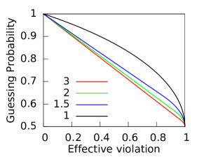
(a) (b)

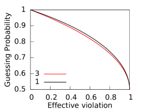
Figure 3: (a) Guessing probability (and simultaneously the tight analogs of monogamies in Theorem 3) for $i=2$ as a function of $(\widetilde{I}_{AB}^{\alpha}-2\alpha)/2(\sqrt{1+\alpha^{2}}-\alpha)$ for various values of $\alpha$. All curves were found using two methods. First, we maximized the guessing probability for a given value of $\widetilde{I}_{AB}^{\alpha}$ over two-ququart states and one-ququart dichotomic measurements. Then, we used the hierarchy of Ref. NPA and with its third level we arrived at curves that coincide with those obtained with the first method with precision $10^{-7}$. For comparison (b) presents the corresponding nontight monogamies proven in theorem 3 ($i=2$) for $\alpha=1,3$ (the curves for $\alpha=1.5,2$ fall in between these two). The black curve is the same on both plots.

Let us finally notice that the quantum elemental monogamies impose the following upper bounds on the guessing probability

$$\max_{j}p(X_{i}=j)\leq\frac{1}{2}\{1+[1+\alpha^{2}-(\widetilde{I}_{AB}^{\alpha}/2)^{2}]^{1/2}\}$$ (44)

with $X=A,B$, $i=1,2$, and $\alpha\geq 1$. This bound was already derived in Ref. AMP , and, as already said, it is tight only for $i=1$. In the case $i=2$, we determined the tight bounds numerically for few $\alpha$s and they are presented in Fig. 3.

III Appendix B: Randomness amplification

Let us begin with recalling the description of the Santha–Vazirani (SV) source (or the $\varepsilon$–source). Its working is defined as follows: it produces a sequence $y_{1},y_{2},\cdots,y_{n}$ of bits according to

$$\tfrac{1}{2}-\varepsilon\leq p(y_{k}|w)\leq\tfrac{1}{2}+\varepsilon\quad(k=1,\ldots,n),$$ (45)

where $w$ denotes any space-time variable that could be the cause of $y_{k}$. In particular, $y_{k}$ can depend on $y_{1},\ldots,y_{k-1}$.

Let now $W$ be any random variable used by an adversary to control the $\varepsilon$-sources and the physical systems held by the parties. The random variable can be thought of a device, held by a villain $E$, with a knob that when set to a particular value $w$ of $W$ makes (i) the SV sources produce bits with certain probabilities obeying (45) and (ii) the devices held by the parties generate a concrete nonsignalling probability distribution represented by $\{p(\boldsymbol{a}|\boldsymbol{x},w)\}_{\boldsymbol{a},\boldsymbol{x}}$. Let us then by $\{p(a_{k},w|\boldsymbol{x})\}_{a_{k},w}$ denote correlations between outcomes obtained by party $k$ and the random variable $W$ for a particular choice of measurement settings $\boldsymbol{x}$. Also, let $\{\widetilde{p}(a)\}$ be the one-party uniform probability distribution, i.e., $\widetilde{p}(a)=1/d$ for any $a$. Introducing then the variational distance

$$D(\{p(x)\},\{q(x)\})=\frac{1}{2}\sum_{x}|p(x)-q(x)|$$ (46)

between two probability distributions $\{p(x)\}$ and $\{q(x)\}$, we can prove the following.

Theorem 4.

Let for any $w$, $\{p(\boldsymbol{a}|\boldsymbol{x},w)\}_{\boldsymbol{a},\boldsymbol{x}}$ be an $N$-partite nonsignalling probability distribution. Then for any $k=1,\ldots,N$ and any choice of measurement settings $\boldsymbol{x}$:

$$D(\{p(a_{k},w|\boldsymbol{x})\}_{a_{k},w},\{\widetilde{p}(a_{k})p(w|\boldsymbol{x})\}_{a_{k},w})$$

$$\hskip 14.22636pt=\frac{1}{2}\sum_{a_{k},w}\left|p(a_{k},w|\boldsymbol{x})-\widetilde{p}(a_{k})p(w|\boldsymbol{x})\right|$$

$$\hskip 14.22636pt\leq\frac{(d-1)^{2}+1}{2d}\,Q_{M}(\boldsymbol{x})I^{N,M,d}_{\mathsf{A}},$$ (47)

where $I^{N,M,d}_{\mathsf{A}}$ is taken in the probability distribution observed by the parties $\{p(\boldsymbol{a}|\boldsymbol{x})\}$. Then

$$Q_{M}(\boldsymbol{x})=\max_{w}\left[\frac{p(w|\boldsymbol{x})}{p_{\min}(w)}\right],$$ (48)

where $p_{\min}(w)=\min_{\boldsymbol{x}}\{p(w|\boldsymbol{x})\}$ with the minimum taken over all measurement settings $\boldsymbol{x}$ appearing in the Bell inequality (24).

Proof.

For simplicity, but without any loss of generality, we prove this theorem for the bipartite case. The generalization to the multipartite case is straightforward.

As before, we denote the parties by $A$ and $B$, while the adversary by $E$. Then, the corresponding inputs and outputs are denoted by $x$, $y$, $z$, and $a$, $b$, and $e$, respectively.

Let us start by noting that for any probability distribution $\{p(a,b|x,y,w)\}_{a,b,x,y}$, the maximal probability of local outcomes obtained by any of the parties, say for simplicity Alice, must obey the inequalities on the guessing probability [see Ineq. (7) in the main text]. That is

$$\max_{a}p(a|x,w)\leq\frac{1}{d}\left(1+I^{2,M,d}_{w}\right)$$ (49)

for any $x=1,\ldots,M$, where by $I_{w}^{2,M,d}$ we have denoted the value of the Bell expression (16) computed for the probability distribution $\{p(a,b|x,y,w)\}_{a,b,x,y}$. Clearly, this bound holds also for any $p(a|x,w)$ which together with the normalization

$$p(a|x,w)=1-\sum_{\alpha\neq a}p(\alpha|x,w),$$ (50)

means that $p(a|x,w)\geq(1/d)[1-(d-1)I^{2,M,d}_{w}]$, and therefore the inequality

$$\left|p(a|x,w)-\frac{1}{d}\right|\leq\frac{d-1}{d}I_{w}^{2,M,d}$$ (51)

holds for any $a$ and $x$. Using then the inequality (49) for $\max_{a}p(a|x,w)$ and (51) for the rest of $p(a|x,w)$, we obtain that for any strategy $w$ and a measurement setting $x$,

$$D(\{p(a|x,w)\}_{a},\{\widetilde{p}(a)\}) = \frac{1}{2}\sum_{a}\left|p(a|x,w)-\widetilde{p}(a)\right|$$ (52)

$$\leq \frac{(d-1)^{2}+1}{2d}I_{w}^{2,M,d}.$$

The remainder of the proof goes along exactly the same lines as in Ref. collbeck-renner , however, for completeness, we will recall it here.

Due to the fact that the observers do not have access to the variable $W$, one has to average Ineq. (52) over the probability distribution $\{p(w|x,y)\}_{w}$ for a particular choice of measurements $x$ and $y$. Together with the facts that $p(a|x,w)=p(a|x,y,w)$ (no-signalling) and $p(w|x,y)p(a|x,y,w)=p(a,w|x,y)$, this allows one to write

$$D(\{p(a,w|x,y)\}_{a,w},\{\widetilde{p}(a)p(w|x,y)\}_{a,w})$$

$$=\frac{1}{2}\sum_{a,w}\left|p(a,w|x,y)-\widetilde{p}(a)p(w|x,y)\right|$$

$$\leq\frac{(d-1)^{2}+1}{2d}\sum_{w}p(w|x,y)I^{2,M,d}_{w}$$ (53)

Let us now concentrate on the right-and side of Ineq. (III). By using Eq. (16), we can bound it from above in the following way

$$\sum_{w}p(w|x,y)I^{2,M,d}_{w}=$$

$$\sum_{w,\alpha}p(w|x,y)(\langle[A_{\alpha}-B_{\alpha}]\rangle_{w}+\langle[B_{\alpha}-A_{\alpha+1}]\rangle_{w})$$

$$=\sum_{w,\alpha}\left(p(w|\alpha,\alpha)\frac{p(w|x,y)}{p(w|\alpha,\alpha)}\langle[A_{\alpha}-B_{\alpha}]\rangle_{w}\right.$$

$$\hskip 42.67912pt+\left.p(w|\alpha+1,\alpha)\frac{p(w|x,y)}{p(w|\alpha+1,\alpha)}\langle[B_{\alpha}-A_{\alpha+1}]\rangle_{w}\right)$$

$$\leq Q_{M}(x,y)\sum_{w,\alpha}\left[p(w|\alpha,\alpha)\langle[A_{\alpha}-B_{\alpha}]\rangle_{w}\right.$$

$$\hskip 71.13188pt+\left.p(w|\alpha+1,\alpha)\langle[B_{\alpha}-A_{\alpha+1}]\rangle_{w}\right]$$

$$=Q_{M}(x,y)\sum_{\alpha}(\langle[A_{\alpha}-B_{\alpha}]\rangle+\langle[B_{\alpha}-A_{\alpha+1}]\rangle)$$

$$=Q_{M}(x,y)I^{2,M,d}_{AB},$$ (54)

where the subscript $w$ in the expectation values $\langle[A_{\alpha}-B_{\alpha}]\rangle_{w}$ and $\langle[B_{\alpha}-A_{\alpha+1}]\rangle_{w}$ means that they are computed for the probability distribution $\{p(a,b|x,y,w)\}_{a,b,x,y}$, and also the convention $p(M+1,M|w)\equiv p(1,M|w)$ is used. Then, $I^{2,M,d}_{AB}$ is computed for the probability distribution $\{p(a,b|x,y)\}$ observed by $A$ and $B$.

By substituting Ineq. (III) to Ineq. (III), one finally obtains Ineq. (4), completing the proof. ∎

One then recovers the inequality of Ref. collbeck-renner from Ineq. (4) by exploiting the fact that $[(d-1)^{2}+1]/d\leq d-1$ $(d\geq 2)$. Let us also notice that one can derive Ineq. (4) using a slightly different approach, which, for completeness, we present below.

Theorem 5.

Let $\{p(\boldsymbol{a}|\boldsymbol{x},w)\}_{\boldsymbol{a},\boldsymbol{x}}$ be a nonsignalling probability distribution for any $w$ and let the probabilities $p(\boldsymbol{x})$ be all equal. Then for any $k=1,\ldots,N$ and any choice of measurement settings $\boldsymbol{x}$:

$$D(\{p(a_{k},w|\boldsymbol{x})\}_{a_{k},w},\{\widetilde{p}(a_{k})p(w|\boldsymbol{x})\}_{a_{k},w})$$

$$\hskip 14.22636pt=\frac{1}{2}\sum_{a_{k},w}\left|p(a_{k},w|\boldsymbol{x})-\widetilde{p}(a_{k})p(w|\boldsymbol{x})\right|$$

$$\hskip 14.22636pt\leq\frac{(d-1)^{2}+1}{2d}\,\widetilde{Q}_{M}(\boldsymbol{x})I^{N,M,d}_{\mathsf{A}},$$ (55)

where $I^{N,M,d}_{\mathsf{A}}$ is taken in the probability distribution observed by the parties $\{p(\boldsymbol{a}|\boldsymbol{x})\}$ and

$$\widetilde{Q}_{M}(\boldsymbol{x})=\max_{w}\left[\frac{p(\boldsymbol{x}|w)}{\widetilde{p}_{\min}(w)}\right],$$ (56)

where $\widetilde{p}_{\min}(w)=\min_{\boldsymbol{x}}\{p(\boldsymbol{x}|w)\}$ with the minimum taken over all measurement settings $\boldsymbol{x}$ appearing in the Bell inequality (24).

Proof.

For simplicity but without any loss of generality, we prove this theorem for the bipartite case. The generalization to the multipartite case is straightforward.

As before, we denote the parties by $A$ and $B$, while the adversary by $E$. Then, the corresponding inputs and outputs are denoted by $x$, $y$, $z$, and $a$, $b$, and $e$, respectively.

Let us start by noting that, by analogy to the case considered in the main text [see Ineq. (6) there], for any $w$, the probability distribution $\{p(a,b|x,y,w)\}_{a,b,x,y}$ satisfies the following monogamy relations

$$\frac{I_{w}^{2,M,d}}{\widetilde{p}_{\min}(w)}+1\geq dp(X_{i}=E_{j}|w)\qquad(X=A,B)$$ (57)

for any pair $\{i,j\}$ $(i,j=1,\ldots,M)$. In the above

$$I_{w}^{2,M,d} = \sum_{\alpha=1}^{M}[p(\alpha,\alpha|w)\langle[A_{\alpha}-B_{\alpha}]\rangle_{w}$$ (58)

$$\hskip 14.22636pt+p(\alpha+1,\alpha|w)\langle[B_{\alpha}-A_{\alpha+1}]\rangle_{w}],$$

is a modified BKP Bell expression taking into account that the inputs $x,y$ are generated with the biased probabilities $p(x,y|w)$, all correlators $\langle[A_{\alpha}-B_{\alpha}]\rangle_{w}$ and $\langle[B_{\alpha}-A_{\alpha+1}]\rangle_{w}$ are computed for the distribution $\{p(a,b|x,y,w)\}_{a,b,x,y}$, and now

$$\widetilde{p}_{\min}(w)=\min_{\alpha=1,\ldots,M}\{p(\alpha,\alpha|w),p(\alpha+1,\alpha|w)\},$$ (59)

where the convention $p(M+1,M|w)\equiv p(1,M|w)$ is used.

The monogamy relations (57) imply (see the main text for the argument in favor of this fact) the bound on the probability of the adversary when using the strategy $w$ to guess the outcomes of any of the measurements performed by one of the parties, say for concreteness Alice (but the same bound holds for outcomes of party $B$):

$$\max_{a}p(a|x,w)\leq\frac{1}{d}\left(1+\frac{I^{2,M,d}_{w}}{\widetilde{p}_{\min}(w)}\right)\quad(x=1,\ldots,M).$$ (60)

Clearly, this bound holds also for any $p(a|x,w)$ which together with the normalization

$$p(a|x,w)=1-\sum_{\alpha\neq a}p(\alpha|x,w),$$ (61)

mean that $p(a|x,w)\geq(1/d)-(d-1)(I^{2,M,d}_{w}/d\widetilde{p}_{\min}(w))$, and therefore the inequality

$$\left|p(a|x,w)-\frac{1}{d}\right|\leq\frac{d-1}{d}\frac{I_{w}^{2,M,d}}{\widetilde{p}_{\min}(w)}.$$ (62)

holds for any $a$ and $x$. Using then the inequality (60) for $\max_{a}p(a|x,w)$ and (62) for the rest of $p(a|x,w)$, we obtain that for any strategy $w$,

$$D(\{p(a|x,w)\}_{a},\{\widetilde{p}(a)\}) = \frac{1}{2}\sum_{a}|p(a|x,w)-\widetilde{p}(a)|$$ (63)

$$\leq \frac{(d-1)^{2}+1}{2d}\frac{I_{w}^{2,M,d}}{\widetilde{p}_{\min}(w)}.$$

Now, since the parties do not have access to $W$, one needs further to average Ineq. (63) over the probability distribution $\{p(w|x,y)\}_{w}$ for a particular choice of measurements $x$ and $y$. This, together with the facts that $p(a|x,w)=p(a|x,y,w)$ (no-signalling) and $p(w|x,y)=p(x,y|w)p(w)/p(x,y)$ implying that $p(w|x,y)p(a|x,y,w)=p(a,w|x,y)$, allows one to write

$$D(\{p(a,w|x,y)\}_{a,w},\{\widetilde{p}(a)p(w|x,y)\}_{a,w})$$

$$=\frac{1}{2}\sum_{a,w}\left|p(a,w|x,y)-\widetilde{p}(a)p(w|x,y)\right|$$

$$\leq\frac{(d-1)^{2}+1}{2d}\sum_{w}\frac{p(x,y|w)}{\widetilde{p}_{\min}(w)}\frac{p(w)}{p(x,y)}I^{2,M,d}_{w}$$

$$\leq\frac{(d-1)^{2}+1}{2d}\widetilde{Q}_{M}(x,y)\sum_{w}\frac{p(w)}{p(x,y)}I^{2,M,d}_{w},$$ (64)

with $\widetilde{Q}_{M}(x,y)=\max_{w}\left[p(x,y|w)/\widetilde{p}_{\min}(w)\right].$ In order to obtain Ineq. (5) from Ineq. (III) it is enough to notice that

$$p(a,b|x,y)=\sum_{w}p(w|x,y)p(a,b|x,y,w)$$ (65)

which, with the aid of the assumption that all the probabilities $p(x,y)$ are equal, further translates to

$$I^{2,M,d}_{AB}=\sum_{w}\frac{p(w)}{p(x,y)}I^{2,M,d}_{w},$$ (66)

where $I^{2,M,d}_{AB}$ is computed for the observed probability distribution $\{p(a,b|x,y)\}$ and the probabilities $p(x,y)=\sum_{w}p(w)p(x,y|w)$ are assumed to be equal for all $x,y$. This completes the proof. ∎

Let us finally notice that under the assumption, which we make above, that all $p(x,y)$ are equal, it holds that $Q_{M}(\boldsymbol{x})=\widetilde{Q}_{M}(\boldsymbol{x})$.

References

(1)R. Horodecki, M. Horodecki, P. Horodecki, and
K. Horodecki, Rev. Mod. Phys. 81, 865 (2009).
(2)N. Brunner et al., Rev. Mod. Phys. 86, 419
(2014).
(3)J. S. Bell, Physics 1, 195 (1964).
(4)H. Buhrman, R. Cleve, S. Massar, and R. de Wolf,
Rev. Mod. Phys. 82, 665 (2010).
(5)A. K. Ekert, Phys. Rev. Lett. 67, 661 (1991);
J. Barrett, L. Hardy, and A. Kent, Phys. Rev. Lett. 95, 010503 (2005);
A. Acín et al., Phys. Rev. Lett. 98, 230501 (2007).
(6)V. Coffman, J. Kundu, and W. K. Wootters,
Phys. Rev. A 61, 052306 (2000).
(7) Ll. Masanes, A. Acín, and N. Gisin, Phys. Rev.
A 73, 012112 (2006).
(8)J. Barrett et al., Phys. Rev. A 71, 022101
(2005).
(9) J. Barrett, A. Kent, S. Pironio, Phys. Rev. Lett. 97, 170409
(2006).
(10)L. Aolita, R. Gallego, A. Cabello, and A. Acín,
Phys. Rev. Lett. 108, 100401 (2012).
(11) B. Toner, F. Verstraete, arXiv:quant-ph/0611001.
(12) B. Toner, Proc. R. Soc. A 465, 59 (2009).
(13) J. F. Clauser, M. A. Horne, A. Shimony, and R. A.
Holt, Phys. Rev. Lett. 23, 880 (1969).
(14) M. Pawłowski, Č. Brukner, Phys. Rev. Lett. 102,
030403 (2009).
(15)P. Kurzyński et al.,
Phys. Rev. Lett. 106, 180402 (2011).
(16)T. R. de Oliveira, A. Saguia, and M. S. Sarandy, Europhys. Lett.
100, 60004 (2012).
(17) A. Acín, N. Brunner, N. Gisin, S. Massar,
S. Pionio, and V. Scarani, Phys. Rev. Lett. 98, 230501,
(2007).
(18) S. Pironio et al., Nature 464, 1021, (2010).
(19) R. Colbeck and R. Renner, Nature Phys.
8, 450 (2012).
(20) A. Grudka et al., arXiv:1303.5591.
(21) R. Gallego et al.,
arXiv:1210.6514v1.
(22) A. Acín, S. Massar, and S. Pironio, Phys. Rev. Lett.
108, 100402 (2012).
(23)S. L. Braunstein and C. Caves, Ann. Phys.
202, 22 (1990).
(24)D. Collins et al., Phys. Rev. Lett. 88,
040404 (2002).
(25) See Supplemental Material for the proof.
(26) M. Pawłowski, Phys. Rev. A 82, 032313, (2010).
(27)R. Horodecki, P. Horodecki, and M. Horodecki, Phys. Lett. A
200, 340 (1995).
(28)Ll. Masanes, quant-ph/0512100.
(29)S. Pironio, Ll. Masanes, A. Leverrier, and A. Acín, Phys.
Rev. X 3, 031007 (2013).