Onsager–Kraichnan Condensation in Decaying Two-Dimensional Quantum Turbulence

Abstract

Despite the prominence of Onsager’s point-vortex model as a statistical description of 2D classical turbulence, a first-principles development of the model for a realistic superfluid has remained an open problem. Here we develop a mapping of a system of quantum vortices described by the homogeneous 2D Gross-Pitaevskii equation (GPE) to the point-vortex model, enabling Monte-Carlo sampling of the vortex microcanonical ensemble. We use this approach to survey the full range of vortex states in a 2D superfluid, from the vortex-dipole gas at positive temperature to negative-temperature states exhibiting both macroscopic vortex clustering and kinetic energy condensation, which we term an Onsager-Kraichnan condensate (OKC). Damped GPE simulations reveal that such OKC states can emerge dynamically, via aggregation of small-scale clusters into giant OKC-clusters, as the end states of decaying 2D quantum turbulence in a compressible, finite-temperature superfluid. These statistical equilibrium states should be accessible in atomic Bose-Einstein condensate experiments.

The importance of the point-vortex model as a statistical description of two-dimensional (2D) classical hydrodynamic turbulence was identified by Onsager Onsager (1949), who predicted that the bounded phase-space of a system of vortices implies the existence of negative-temperature states exhibiting clustering of like-circulation vortices Eyink and Sreenivasan (2006). This model provides great insight into 2D classical turbulence (CT) Boffetta and Ecke (2012), and much subsequent work has focused on the point-vortex model as an approximate statistical description of decaying 2DCT Tabeling (2002); Montgomery and Joyce (1974); Montgomery et al. (1992); Miller (1990); Robert and Sommeria (1991). While classical fluids cannot directly realize the point-vortex model, atomic Bose-Einstein condensates (BECs) — which present an emerging theoretical Parker and Adams (2005); Nazarenko and Onorato (2007); Horng et al. (2009); Numasato and Tsubota (2010); Numasato et al. (2010); Sasaki et al. (2010); White et al. (2010); Nowak et al. (2011, 2012); Schole et al. (2012); Bradley and Anderson (2012); White et al. (2012); Kusumura et al. (2013); Tsubota et al. (2013); Reeves et al. (2013) and experimental Neely et al. (2010, 2013); Wilson et al. (2013) paradigm system for the study of quantum vortices and 2D quantum turbulence (2DQT) — offer the possibility of physically realizing Onsager’s negative-temperature equilibrium states. A concrete realization of the point-vortex model in an atomic superfluid will broaden our understanding of the universality of 2D turbulence by enabling new studies of spectral condensation of energy at large scales Kraichnan (1975); Kraichnan and Montgomery (1980); Chertkov et al. (2007); Xia et al. (2008), statistical mechanics of negative-temperature states Weiss and McWilliams (1991); Campbell and O’Neil (1991); Sano et al. (2007), the dynamics of macroscopic vortex clustering Yatsuyanagi et al. (2005), and the inverse energy cascade Siggia and Aref (1981); Kraichnan (1967); Leith (1968); Batchelor (1969), previously confined to 2DCT.

In this letter we develop an analytic statistical description of the microstates of 2D quantum vortices within the homogeneous Gross-Pitaevskii theory, and show that macroscopically clustered vortex states emerge from small-scale initial clustering as end products of decaying 2DQT. As in CT, the homogeneous system offers the clearest insight into the underlying physics, and is increasingly relevant experimentally Gaunt et al. (2013). Consequently, our results describe physics relevant to a wide range of possible vortex experiments in atomic BECs. By systematically sampling the microcanonical ensemble for the vortex degrees of freedom, we give a detailed, unifying view of the properties of vortex matter in a homogeneous 2D superfluid. We characterize the emergence of macroscopic clusters of quantum vortices at negative temperatures, linked with spectral condensation of energy at the system scale. In the context of 2DQT we call this the Onsager–Kraichnan condensate (OKC), as it represents a physically realizable state that unifies Onsager’s negative-temperature point-vortex clusters with the spectral condensation of kinetic energy predicted in 2DCT by Kraichnan Kraichnan (1975).

Atomic BECs support quantum vortices subject to thermal and acoustic dissipative processes that may be detrimental to the observation of an OKC. We assess the accessibility of the excited states comprising an OKC via dynamical simulations according to the damped Gross-Pitaevskii equation (dGPE). We find that our statistical approach describes the end-states of decaying 2DQT that emerge dynamically from low-entropy initial states. Even for relatively small positive point-vortex energies, the OKC emerges as a result of statistically driven transfer of energy to large length scales.

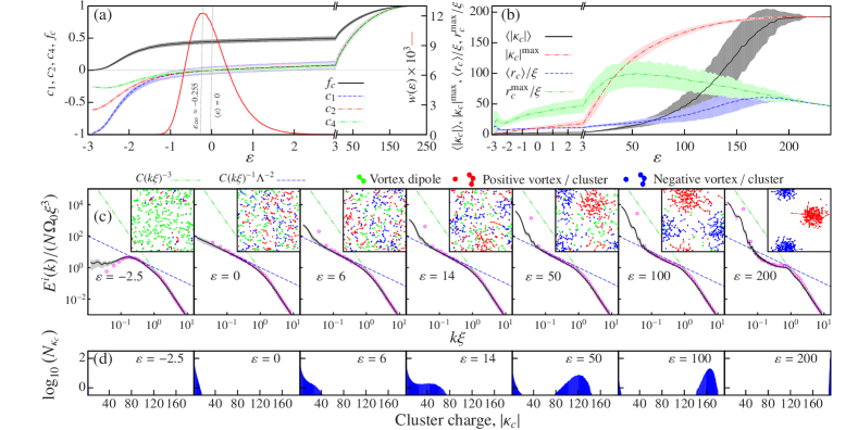
Figure 1: (color online). Properties of neutral $N$-vortex states in statistical equilibrium, corresponding to the end-states of decaying 2DQT. (a): Clustering measures $f_{c}$ and $c_{B}$ and structure function $w(\varepsilon)$; vertical grey lines indicate the expected energy ($\langle\varepsilon\rangle$) and the boundary between positive- and negative-temperature states ($\varepsilon_{\infty}$). (b): Average and maximum cluster charges ($|\kappa_{c}|$) and radii ($r_{c}$) obtained using the RCA (see text). (c): IKE spectrum in the point-vortex-like approximation [Eq. (3)] (solid black line, grey shaded area), and obtained from the GPE wavefunctions Bradley and Anderson (2012); Numasato et al. (2010) (magenta circles). Straight lines show analytical $k^{-3}$ and $k^{-1}$ power laws (see text). Inset: typical vortex configurations (field of view $L\times L$): dots indicate vortices, which have been sorted into dipoles, free vortices and clusters by the RCA (see legend). Lines show the minimal spanning tree of clusters and identify dipoles. (d): Distribution of $N_{\kappa_{c}}$. Shaded areas behind curves in (a,b,c) indicate the width of the equilibrium distribution ($\pm 1$ standard deviations). Ensemble sizes are given in sam .

To map the Gross-Pitaevskii theory to the point-vortex model, we introduce an ansatz wavefunction for $N$ vortices in a homogeneous periodic square BEC of side $L$, with positions $\mathbf{r}_{j}$ and circulations $h\kappa_{j}/m$ defined by charges $\kappa_{j}=\pm 1$ ($\sum_{j=1}^{N}\kappa_{j}=0$),

$$\psi(\mathbf{r},\{\mathbf{r}_{j}\},\{\kappa_{j}\})=e^{i\theta(\mathbf{r},\{\mathbf{r}_{j}\},\{\kappa_{j}\})}\prod_{p=1}^{N}\chi\left(|\mathbf{r}-\mathbf{r}_{p}|\right)\,,$$ (1)

where $\chi(r)$ is the radial profile of an isolated quantum vortex core, obtained numerically Bradley and Anderson (2012). Unlike the velocity field for point-vortices in a doubly-periodic domain Campbell and O’Neil (1991); Weiss and McWilliams (1991), the associated quantum phase $\theta$ does not, to our knowledge, appear in the literature. We present an expression for $\theta$ as a rapidly convergent sum, obtained from a poorly convergent sum over periodic replica vortices, in the Supplemental Material sup . The phase $\theta$ yields a periodic superfluid velocity $\mathbf{v}=(\hbar/m)\nabla\theta$ very close to the point-vortex velocity, but consistently modified by the boundary conditions such that $\theta(x+\eta_{x}L,y+\eta_{y}L)=\theta(x,y)+\zeta 2\pi$, for all $\eta_{x},\eta_{y},\zeta\in\mathbb{Z}$, remains a well-defined quantum phase. To ensure that $\chi(r)$ is accurate, we enforce a minimum-separation constraint $|\mathbf{r}_{p}-\mathbf{r}_{q}|\geq 2\pi\xi$, where $\xi=\hbar/\sqrt{\mu m}$ is the healing length (for BEC chemical potential $\mu$ and atomic mass $m$), and $1\leq p\neq q\leq N$.

Up to an additive constant, the total kinetic energy in the point-vortex model is $N\Omega_{0}\xi^{2}\varepsilon(\{\mathbf{r}_{j}\},\{\kappa_{j}\})$. Here, the dimensionless point-vortex energy (per vortex) is given by Campbell and O’Neil (1991)

$$\varepsilon(\{\mathbf{r}_{j}\},\{\kappa_{j}\})=\frac{1}{N}\sum_{p=1}^{N-1}\sum_{q=p+1}^{N}\kappa_{p}\kappa_{q}f\left(\frac{\mathbf{r}_{p}-\mathbf{r}_{q}}{L}\right)\,,$$ (2)

where $f(\mathbf{r})\equiv f(x,y)=2\pi[|y|(|y|-1)+1/6]-\log\{\prod_{s=-\infty}^{\infty}[1-2\cos(2\pi x)\exp(-2\pi|y+s|)+\exp(-4\pi|y+s|)]\}$, and $\Omega_{0}=\pi\hbar^{2}n_{0}/m\xi^{2}$ is the unit of enstrophy for 2D homogeneous superfluid density $n_{0}$ Bradley and Anderson (2012). Accounting for compressible effects with the core ansatz $\chi_{\Lambda}(r)=[n_{0}r^{2}/(r^{2}+\xi^{2}\Lambda^{-2})]^{1/2}$, the incompressible kinetic energy (IKE) spectrum of Eq. (1) at scales below the system size $L$ is well approximated by sup ; Bradley and Anderson (2012)

$$E^{i}(k)=\Omega_{0}\xi^{3}F_{\Lambda}(k\xi)\left[N+2\sum_{p=1}^{N-1}\sum_{q=p+1}^{N}\kappa_{p}\kappa_{q}J_{0}(k|\mathbf{r}_{p}-\mathbf{r}_{q}|)\right]\,,$$ (3)

where $F_{\Lambda}(k\xi)=\Lambda^{-1}g(k\xi\Lambda^{-1})$, $g(z)=(z/4)[I_{1}(z/2)K_{0}(z/2)-I_{0}(z/2)K_{1}(z/2)]$, $\Lambda=\xi^{2}n_{0}^{-1/2}d\chi(0)/dr\approx 0.825$ and $J_{\alpha}$ ($I_{\alpha}$, $K_{\alpha}$) are (modified) Bessel functions. Equation (3) leads to a universal ultraviolet (UV, $k\gg\xi^{-1}$) $k^{-3}$ power-law, $E^{i}(k)=C(k\xi)^{-3}$, where $C=\Lambda^{2}{N\Omega_{0}\xi^{3}}$ Bradley and Anderson (2012); Nowak et al. (2012). In the infrared (IR, $k\lesssim\xi^{-1}$) the average spectrum of $N$-vortex configurations with randomly distributed vortices is equal to the sum of $N$ independent single-vortex spectra, giving the $k^{-1}$ power-law $E^{i}(k)=C(k\xi)^{-1}/\Lambda^{2}$ Kusumura et al. (2013); Bradley and Anderson (2012); Nowak et al. (2012).

The wavefunction $\psi$ [Eq. (1)] is set entirely by the vortex configuration, allowing us to adopt a statistical treatment where, for each configuration ($\{\mathbf{r}_{j}\}$,$\{\kappa_{j}\}$), $\psi$ defines a microstate of the 2D BEC 2db . Aside from the minimum-separation constraint, the phase $\theta$ in Eq. (1) establishes a one-to-one correspondence between the $N$-vortex states of a 2D BEC and the microstates of the classical point-vortex model. The set of all microstates $\psi$ at fixed point-vortex energy $\varepsilon$ [Eq. (2)] defines a microcanonical ensemble; the measure of this set is the structure function $W(\varepsilon)$ [which defines the system entropy $S(\varepsilon)=k_{B}\ln(W(\varepsilon))$]. The normalized structure function, $w(\varepsilon)\equiv W(\varepsilon)(\int d\varepsilon W(\varepsilon))^{-1}$, is obtained numerically as a histogram of $\varepsilon$ for random vortex configurations. We sample the microcanonical ensemble at energy $\varepsilon$ numerically, using a random walk to generate many $N$-vortex configurations having energies within a given tolerance sam . Related microcanonical sampling techniques have previously been applied to the classical point-vortex model Campbell and O’Neil (1991); Weiss and McWilliams (1991); Yatsuyanagi et al. (2005); Sano et al. (2007). Averages of observables over this ensemble are dominated by the most likely (highest-entropy) configurations. For large $N$ (ensuring ergodicity Weiss and McWilliams (1991); Campbell and O’Neil (1991)) ensemble averages define a statistical equilibrium corresponding to time-averaged properties of the end-states of decaying quantum vortex turbulence at energy $\varepsilon$.

To demonstrate that quantum vortices in a 2D BEC can provide a physical realization of negative-temperature states exhibiting macroscopic vortex clustering, we sample the GPE microstates of the 2D BEC, compute the IKE spectrum, and decompose the vortex configurations into dipoles and clusters using the recursive cluster algorithm (RCA) developed in Ref. Reeves et al. (2013). For each cluster the RCA yields the cluster charge $\kappa_{c}$ and average radius $r_{c}$ (average distance of constituent vortices from the cluster center of mass). We define the clustered fraction $f_{c}=\sum_{s}|\kappa_{c,s}|/N$, where $\kappa_{c,s}$ is the charge of the $s$th cluster. We also define $N_{\kappa_{c}}$ as the total number of vortices participating in all clusters of charge $\pm|\kappa_{c}|$. Finally, we introduce the correlation functions $c_{B}=\sum_{p=1}^{N}\sum_{q=1}^{B}\kappa_{p}\kappa^{(q)}_{p}/BN$, where $\kappa^{(q)}_{p}$ is the charge of the $q$th nearest-neighbor to vortex $p$. These are directly related to the functions $C_{B}$ introduced in Ref. White et al. (2012); a value of $c_{B}>0$ ($<0$) indicates (anti-)correlation between vortex charges, up to nearest neighbours of $B$th order.

Figure 1(a) shows $w(\varepsilon)$ for $N=384$ vortices in a doubly periodic box of side $L=512\xi$. The boundary between positive- and negative-temperature states, $\varepsilon_{\infty}$, lies at the maximum of $W(\varepsilon)$, where the temperature $T=W(\partial W/\partial\varepsilon)^{-1}/k_{B}\rightarrow\infty$. We find $\varepsilon_{\infty}\approx-0.255$ and the mean energy $\langle\varepsilon\rangle=0$ known from the point-vortex model Campbell and O’Neil (1991) despite the minimum-separation constraint. Figure 1 also shows the averages of the clustering measures [Fig. 1(a,b)], the IKE spectrum [Fig. 1(c)], and the distribution of $N_{\kappa_{c}}$ [Fig. 1(d)] as a function of $\varepsilon$. At $\varepsilon=0$, $c_{B}$ ($f_{c}$) is equal to $0$ ($1/2$), indicating an uncorrelated vortex distribution. The distribution of $N_{\kappa_{c}}$ is strongly skewed towards small clusters, with $|\kappa_{c}|^{\rm max}<20$ and $r_{c}^{\rm max}<50\xi\ll L$, and the IKE spectrum follows the $k^{-1}$ law in the IR-region. At energies $\varepsilon<0$ (where $T>0$ for $\varepsilon\leq\varepsilon_{\infty}$), $c_{B}$ ($f_{c}$) drops below $0$ ($1/2$), indicating proliferation of vortex dipoles and reduced number, charge, and radius of vortex clusters. As $\varepsilon\rightarrow-3$ one obtains a vortex-dipole gas with approximately the minimal spacing $2\pi\xi$ [see Fig. 2(a)]. The IKE spectrum lies below the $k^{-1}$ law at large scales. At energies $\varepsilon>0$ (where $T<0$) Fig. 1 shows macroscopic vortex clustering and spectral condensation of IKE. While low-order measures of clustering ($c_{B}$, $f_{c}$) increase slowly with $\varepsilon$, the distribution of vortices bifurcates, revealing the appearance of two (opposite-sign) macroscopic clusters. Spectrally, the energy associated with these clusters manifests itself as an OKC lying above the $k^{-1}$ power-law at large scales. The charge and radius of clusters ($|\kappa_{c}|^{\rm max}$ and $r_{c}^{\rm max}$) grows more rapidly with $\varepsilon$ than $\langle|\kappa_{c}|\rangle$ and $\langle r_{c}\rangle$ up to $\varepsilon\sim 50$, highlighting the utility of the RCA for the characterization of point-vortex states. Above this energy, clusters increase in charge less rapidly, and absorb further energy by shrinking in radius. For $\varepsilon\gtrsim 200$ two clusters contain all the vortices, illustrating the phenomenon of supercondensation Kraichnan and Montgomery (1980); in this regime the $k^{-1}$ spectrum vanishes.

In contrast to the UV-divergent point-vortex model, the universal $k^{-3}$ UV asymptotic of the IKE spectrum [Eq. (3)] implies a physical transition energy for the emergence of the OKC, given by $E_{0}\equiv E^{i}_{\rm tot}(\varepsilon=0)$, where $E^{i}_{\rm tot}(\varepsilon)\equiv\int dkE^{i}(k)$. An analytic estimate of $E_{0}$ follows from the second term in Eq. (3) averaging to zero at $\varepsilon=0$ ($c_{B}=0$ for all $B$); correctly accounting for the discrete nature of the spectrum sup yields $E_{0}\approx 4.735N\Omega_{0}\xi^{2}$, in good agreement with the numerical value $E_{0}\approx 4.821N\Omega_{0}\xi^{2}$ obtained from $\psi$, which does not rely on the core ansatz used to obtain Eq. (3). We find that the total IKE is very well predicted by $E^{i}_{\rm tot}(\varepsilon)=E_{0}+\varepsilon N\Omega_{0}\xi^{2}$. Thus, the appearance of the OKC is due to saturation of excited states: IKE exceeding $E_{0}$ accumulates near the system scale, forming the spectral feature lying above the $k^{-1}$ spectrum. Note that the OKC is a (quasi-)equilibrium phenomenon distinct from the classical scenario of condensation in forced turbulence, where the $k^{-5/3}$ spectrum of the inverse energy cascade (IEC) gives way to $k^{-3}$ at low $k$ associated with the dynamical condensate Chertkov et al. (2007); Xia et al. (2008); Chan et al. (2012).

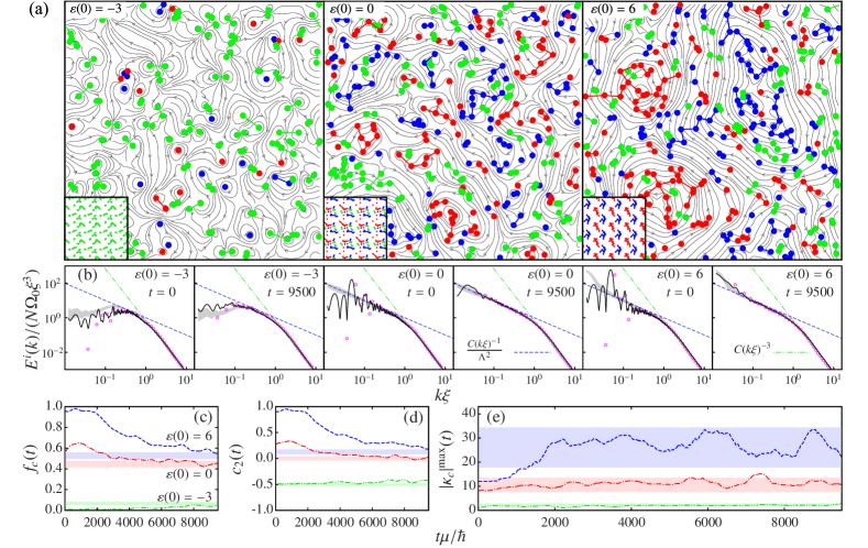
Figure 2: (color online). Dynamical dGPE evolution of non-equilibrium neutral $N$-vortex states towards statistical equilibrium (see also animations in sup ). (a): RCA decomposition after equilibriation ($t=9500\hbar/\mu$), with initial conditions inset. Streamlines show the incompressible velocity field. Field of view is $L\times L$. (b): IKE spectrum, compared to the statistical equilibrium distribution from Fig. 1(c) (grey solid line, thickness indicates $\pm 1$ standard deviations). Other symbols in (a,b) as in Fig. 1(c). (c): Clustered fraction $f_{c}$. (d): Correlation function $c_{2}$. (e): Absolute charge, $|\kappa_{c}|$, of the largest vortex cluster. Spectra and measures are shown as a moving average from $t$ to $t+500\hbar/\mu$, and $E^{i}(k)$ is normalized by $N(t)$; decay of $N(t)$ for $\varepsilon(0)>-3$ is negligible ($\lesssim 5\%$). Horizontal shading in (c–e) shows the statistical equilibrium distributions from Fig. 1(a,b) (shaded areas indicate $\pm 1$ standard deviations). Note that we compare the $\varepsilon(0)=-3$ evolution to the statistical equilibrium at $\varepsilon=-2.5$, since dipole annihilation [for $\varepsilon=-3$, $N(10^{4})=178$] leads to $\varepsilon(10^{4})\approx-2.5$.

To demonstrate that Fig. 1 provides a quantitative description of decaying QT in a 2D BEC, and that statistically-driven transfers of energy to large length scales can occur in a compressible quantum fluid, we consider the dynamics of non-equilibrium states in the dGPE Tsubota et al. (2002); Penckwitt et al. (2002); Blakie et al. (2008). For a 2D BEC (subject to tight harmonic confinement in the $z$-direction with oscillator length $l_{z}$) this can be written as

$$i\hbar\frac{\partial\psi(\mathbf{r},t)}{\partial t}=(1-i\gamma)\left(-\frac{\hbar^{2}\nabla_{\perp}^{2}}{2m}+g_{2}|\psi(\mathbf{r},t)|^{2}-\mu\right)\psi(\mathbf{r},t)\,,$$ (4)

where $g_{2}=\sqrt{8\pi}\hbar^{2}a_{s}/ml_{z}$, $m$ is the atomic mass, and $a_{s}$ is the $s$-wave scattering length. The dimensionless damping rate $\gamma$ describes collisions between condensate atoms and non-condensate atoms, an important physical process in real 2D superfluids that leads to effective viscosity Bradley and Anderson (2012) and suppression of sound energy at high $k$. We use the experimentally realistic value $\gamma=10^{-4}$ Neely et al. (2013) in our simulations. We use a random walk to obtain a neutral configuration of $N^{\prime}=24$ vortices in a periodic box of length $L^{\prime}=128\xi$ at energy $\varepsilon^{\prime}$. A $4^{2}$ tiling of this configuration, with each vortex subject to Gaussian position noise (variance $\xi$), provides a non-equilibrium, low-entropy state of $N=384$ vortices in a box with $L=512\xi$ and energy $\varepsilon$ (found by adjusting $\varepsilon^{\prime}$). This state is then evolved to time $10^{4}\hbar/\mu$ in the dGPE, over which time we find that the compressible energy does not increase [and $\varepsilon(t)$ does not decay] significantly, supporting our statistical description gze .

Figure 2 shows the time evolution of the vortex configuration for three different initial energies [Fig. 2(a)] with IKE spectra [Fig. 2(b)] and clustering measures [Fig. 2(c-e)] determined by short-time averaging of individual runs of the dGPE. While approach to complete equilibrium is slow, Fig. 2(e) shows that the charge of the largest cluster equilibriates more rapidly (by $t\sim 2000\hbar/\mu$). For $\varepsilon(0)=-3$, the dynamics consists largely of dipole-dipole collisions and vortex-antivortex annihilation (increasing the energy per vortex $\varepsilon$, Campbell and O’Neil (1991)), and exhibits a time-invariant IKE spectrum; these positive-temperature point-vortex states have no analog in 2DCT Campbell and O’Neil (1991). For $\varepsilon(0)=0$, the approach to equilibrium involves significant dipole-cluster interactions that redistribute the cluster charges, decreasing $f_{c}$ and $c_{B}$ while increasing $|\kappa_{c}|^{\rm max}$. This redistribution transfers energy to large scales, producing an approximate $k^{-1}$ power-law in the IR [note that the time-averaged spectrum is expected to fluctuate relative to the $10^{4}$-configuration average in Fig. 1(c)]. For $\varepsilon(0)=6$ the dynamics is reminiscent of 2DCT. Energy transfer to large scales builds an OKC, with the vortices grouping into two macroscopic clusters okc . Although a steady $k^{-5/3}$ spectrum is absent (and would require continuous forcing and damping to establish a steady inertial range Reeves et al. (2013)) some intermittent $k^{-5/3}$ behaviour is evident sup . The equilibrium distribution of vortices outside of the OKC closely resembles the uncorrelated ($\varepsilon=0$) state Eyink and Sreenivasan (2006) and has a low level of clustering. As the initial condition contains many small clusters, this counterintuitively causes low-order measures of clustering [$f_{c}$ and $c_{2}$ in Fig. 2(c,d), and all $c_{B}$ for $B\lesssim 10$] to decay during OKC formation. Thus, high-order clustering information provided by the RCA is vital in identifying OKC: the rapid increase of $|\kappa_{c}|^{\rm max}$ for $\varepsilon(0)=6$ in Fig. 2(e) contrasts with the cases $\varepsilon(0)=0,-3$, indicating the emergence of the OKC. The demonstration of a statistically driven transfer of kinetic energy to large scales underpins the existence of an IEC in far-from-equilibrium 2DQT in scenarios with appreciable vortex clustering Bradley and Anderson (2012); Reeves et al. (2013), and is complementary to the direct energy cascade identified in scenarios dominated by vortex-dipole recombination Numasato et al. (2010); Chesler et al. (2013).

We have developed a first-principles realization of Onsager’s point-vortex model in a 2D superfluid, and observe the upscale energy transfer of 2DCT in decaying 2DQT described by the damped Gross-Pitaevskii equation. Configurational analysis of the vortex states and associated energy spectra demonstrate the emergence of an Onsager–Kraichnan condensate of quantum vortices occurring at negative temperatures in equilibrium, and as the end states of decaying 2DQT. The microcanonical sampling approach opens a new direction in the study of 2DQT, enabling systematic studies of far-from-equilibrium dynamics, energy transport, inertial ranges, and other emergent phenomena in 2DQT, and points the way to experimental realization of Onsager–Kraichnan condensation.

Supplemental Material

I I. Construction of the quantum phase of an $N$-vortex wavefunction in a periodic square domain

Here, we construct the phase $\theta(\mathbf{r},\{\mathbf{r}_{j}\},\{\kappa_{j}\})$ associated with an ansatz wavefunction for a neutral system of $N$ superfluid vortices with positions $\mathbf{r}_{j}$ and circulations $h\kappa_{j}/m$ (charges $\kappa_{j}=\pm 1$) in a homogeneous periodic square 2D BEC of side $L$.

The phase associated with the velocity field of a single point-vortex $j$ is given by

$$\theta_{j}=\kappa_{j}\mbox{atan2}(y-y_{j},x-x_{j})\,,$$ (1)

where the four-quadrant arctangent function is defined by

$$\mbox{atan2}(y,x)=\left\{\begin{array}[]{lr}\mathrm{atan}(y/x),&x>0\\ \mathrm{atan}(y/x)+\pi,&x<0,y>0\\ \mathrm{atan}(y/x)-\pi,&x<0,y<0\end{array}\right.$$ (2)

Because we only require $\theta_{j}$ to within an arbitrary multiple of $2\pi$, we may gain a substantial notational convenience by noting that the simplified definition

$$\theta_{j}=\kappa_{j}\mathrm{atan}(y-y_{j},x-x_{j})+\pi H(x-x_{j})\,,$$ (3)

where $H(x)$ is the Heaviside unit-step function, is equivalent to Eq. (1) to within such a multiple. Due to the infinite extent of this phase field, to obtain the phase due to $N$ point-vortices in a doubly-periodic square domain it is necessary to sum over the entire infinite periodic array of vortices (i.e., not only over the periodic unit cell, but over the infinite periodic lattice). Implemented directly, such a summation is poorly convergent. Summing over too few unit cells of the infinite lattice introduces spurious boundary effects at the edge of the central unit cell; in particular the nucleation of undesired extra vortices at the boundaries leading to subsequent large-scale compressible flows. While this problem can be to some extent mitigated by a short evolution in imaginary time, by performing such an evolution one relinquishes control over the exact number and positions of the vortices. However, when computing the phase on a large simulation grid, even for small numbers of vortices ($<10$), we find that summing over a sufficient number of unit cells to eliminate spurious boundary effects is computationally infeasible. In the following we overcome this challenge by analytically reducing the poorly-convergent, doubly-infinite sum to a single convergent summation. The final form for $\theta$ we present allows exact vortex positioning, eliminates boundary effects entirely, and leads to very short computation times even on large grids.

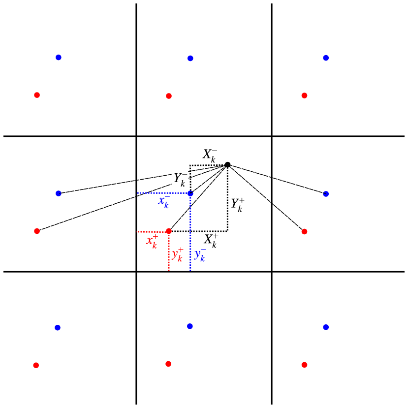
Figure 1: Diagram illustrating summation over the infinite periodic array of vortices corresponding to a single vortex dipole in the unit cell. The black dot indicates a test position $(x,y)$ at which we compute the phase due to the dipole formed by a positive-circulation vortex at $(x_{k}^{+},y_{k}^{+})$ and a negative-circulation vortex at $(x_{k}^{-},y_{k}^{-})$.

We begin by working in a periodic unit cell with coordinates $0\leq x,y<2\pi$ for simplicity (the extension to the general periodic cell $0\leq\tilde{x},\tilde{y}<L$ is straightforward and follows subsequently). Figure 1 illustrates the geometry of the problem for the $k$th vortex dipole (any neutral configuration of $N$ vortices can be arbitrarily partitioned into $N/2$ dipoles). This vortex dipole is formed by a positive vortex located at $(x_{k}^{+},y_{k}^{+})$ and a negative vortex located at $(x_{k}^{-},y_{k}^{-})$. To determine the phase at a test point $(x,y)$ it is convenient to introduce the auxilliary variables $(X_{k}^{+},Y_{k}^{+})=(x-x_{k}^{+},y-y_{k}^{+})$ and $(X_{k}^{-},Y_{k}^{-})=(x-x_{k}^{-},y-y_{k}^{-})$. In the present treatment we shall assume that $|x_{k}^{+}-x_{k}^{-}|,|y_{k}^{+}-y_{k}^{-}|<\pi$; this restriction can always be met by an appropriate translation of the unit cell and provides a considerable notational convenience. However, note that when computing the phase due to a given $N$-vortex configuration it is in fact somewhat easier to follow the procedure developed here for each vortex pair without enforcing this requirement: Instead one can subsequently transform the phase $\theta_{k}$ for each vortex dipole according to $\theta_{k}\rightarrow\theta_{k}-xH(|y_{k}^{+}-y_{k}^{-}|-\pi)+yH(|x_{k}^{+}-x_{k}^{-}|-\pi)$ to obtain the correct result.

We proceed by first reducing the doubly-infinite summation to a singly-infinite one by analytically summing over all periodic replicas of the unit cell in the $x$-direction. Explicitly considering just the central row of unit cells in the figure, we have for periodic replicas of the positive vortex

$$\theta_{k,+}^{(\mathrm{row})}(x,y)=\sum_{m=0}^{\infty}\mathrm{atan}\left(\frac{Y_{k}^{+}}{2\pi m+X_{k}^{+}}\right)-\sum_{m=1}^{\infty}\mathrm{atan}\left(\frac{Y_{k}^{+}}{2\pi m-X_{k}^{+}}\right)\\ +\pi H(X_{k}^{+})+f^{+}(y)\,.$$ (4)

The penultimate term above represents the adjustment to the angle obtained when “passing” a vortex in the $x$-direction [see Eq. (3)]. The final term reflects the fact that the phase is only defined up to a, possibly $y$-dependent, constant. Rearranging the sums in Eq. (4) under a single summation sign we obtain

$$\theta_{k,+}^{(\mathrm{row})}(x,y)=\sum_{m=1}^{\infty}\left[\mathrm{atan}\left(\frac{Y_{k}^{+}}{2\pi m+(X_{k}^{+}-\pi)-\pi}\right)\right.\\ \left.-\mathrm{atan}\left(\frac{Y_{k}^{+}}{2\pi m-(X_{k}^{+}-\pi)-\pi}\right)\right]+\pi H(X_{k}^{+})+f^{+}(y)\,.$$ (5)

This summation can be evaluated using a formula due to Ramanujan Berndt et al. (1981), giving

$$\theta_{k,+}^{(\mathrm{row})}(x,y)=-\mathrm{atan}\left[\tanh\left(\frac{Y_{k}^{+}}{2}\right)\tan\left(\frac{X_{k}^{+}-\pi}{2}\right)\right]\\ +\pi H(X_{k}^{+})+f^{+}(y)\,.$$ (6)

An equivalent treatment for the negative vortex yields

$$\theta_{k,-}^{(\mathrm{row})}(x,y)=\mathrm{atan}\left[\tanh\left(\frac{Y_{k}^{-}}{2}\right)\tan\left(\frac{X_{k}^{-}-\pi}{2}\right)\right]\\ -\pi H(X_{k}^{-})+f^{-}(y)\,.$$ (7)

Summing over all the rows of unit cells (i.e., summing over the $y$-direction) leads to the singly-infinite sum for the total phase due to the dipole and all its periodic replicas

$$\theta_{k}(x,y)=\sum_{n=-\infty}^{\infty}\left\{\mathrm{atan}\left[\tanh\left(\frac{Y_{k}^{-}+2\pi n}{2}\right)\tan\left(\frac{X_{k}^{-}-\pi}{2}\right)\right]\right.\\ \left.-\mathrm{atan}\left[\tanh\left(\frac{Y_{k}^{+}+2\pi n}{2}\right)\tan\left(\frac{X_{k}^{+}-\pi}{2}\right)\right]\right.\\ \left.+\pi\left[H(X_{k}^{+})-H(X_{k}^{-})\right]\vphantom{\tanh\left(\frac{Y_{k}^{-}+2\pi n}{2}\right)}\right\}+f(y)\,,$$ (8)

where $f(y)=f^{+}(y)+f^{-}(y)$. The correct $f(y)$ is determined by the requirement that the phase be periodic in $y$, in the sense that

$$\theta_{k}(x,y+2\pi)=\theta_{k}(x,y)+s2\pi\,,$$ (9)

for integer $s$. Keeping in mind this requirement, we differentiate Eq. (8) w.r.t. $y$, yielding the $y$-component of the velocity field

$${v_{y}}_{k}(x,y)=\frac{1}{2}\sum_{n=-\infty}^{\infty}\left[\frac{-\sin(X_{k}^{+})}{\cos(X_{k}^{+})-\cosh(2n\pi+Y_{k}^{+})}\right.\\ \left.+\frac{\sin(X_{k}^{-})}{\cos(X_{k}^{-})-\cosh(2n\pi+Y_{k}^{-})}\right]+f^{\prime}(y)\,.$$ (10)

Note that this differs from the standard point-vortex result Weiss and McWilliams (1991) only by the term $f^{\prime}(y)$. To obtain appropriate point-vortex physics, we therefore require that $f^{\prime}(y)$ be equal to a constant. Physically, this constant appears because of the restriction [Eq. (9)] that $\theta_{k}$ should be a well-defined quantum phase, a requirement not present in the classical point-vortex model. Equation (10) can be integrated over a single period in $y$ to obtain the change in phase over the unit cell in this direction,

$$\Delta\theta_{k}=\int_{0}^{2\pi}dy{v_{y}}_{k}(x,y)\\ =\frac{1}{2}\int_{-\infty}^{\infty}dy\left[\frac{-\sin(X_{k}^{+})}{\cos(X_{k}^{+})-\cosh(Y_{k}^{+})}\right.\\ \left.+\frac{\sin(X_{k}^{-})}{\cos(X_{k}^{-})-\cosh(Y_{k}^{-})}\right]+\int_{0}^{2\pi}dyf^{\prime}(y)\,,$$ (11)

where we have used the periodicity of ${v_{y}}_{k}$ in order to replace the infinite sum in Eq. (10) with infinite limits in the integral.

Evaluating both integrals, for constant $f^{\prime}(y)$, gives

$$\Delta\theta_{k}=x_{k}^{+}-x_{k}^{-}+2\pi f^{\prime}(y)\,.$$ (12)

Hence, the minimal choice to recover periodicity in $y$ is $f^{\prime}(y)=-(x_{k}^{+}-x_{k}^{-})/2\pi$, yielding the final expression

$$\theta_{k}(x,y)=\sum_{n=-\infty}^{\infty}\left\{\mathrm{atan}\left[\tanh\left(\frac{Y_{k}^{-}+2\pi n}{2}\right)\tan\left(\frac{X_{k}^{-}-\pi}{2}\right)\right]\right.\\ \left.-\mathrm{atan}\left[\tanh\left(\frac{Y_{k}^{+}+2\pi n}{2}\right)\tan\left(\frac{X_{k}^{+}-\pi}{2}\right)\right]\right.\\ \left.+\pi\left[H(X_{k}^{+})-H(X_{k}^{-})\right]\vphantom{\tanh\left(\frac{Y_{k}^{-}+2\pi n}{2}\right)}\right\}-\frac{x_{k}^{+}-x_{k}^{-}}{2\pi}y\,.$$ (13)

In practice the sum in Eq. (13) converges rapidly, such that $\sum_{n=-\infty}^{\infty}\rightarrow\sum_{n=-5}^{5}$ is sufficient.

Using the dipole result above for the case $L=2\pi$, the total phase due to a neutral configuration of $N$ vortices in a periodic box of arbitrary side length $L$, with coordinate system $(\tilde{x},\tilde{y})\equiv\tilde{\mathbf{r}}$, can be obtained by an appropriately scaled sum over all dipoles

$$\theta_{\rm total}(\tilde{x},\tilde{y})=\sum_{k=1}^{N/2}\theta_{k}(x,y)\,,$$ (14)

where $(x,y)=2\pi(\tilde{x},\tilde{y})/L$, and the implicit vortex position arguments to $\theta_{k}$ should also be appropriately scaled (i.e., $\mathbf{r}_{j}=2\pi\tilde{\mathbf{r}}_{j}/L$). We have tested this expression for a wide variety of numbers, $N$, and individual configurations of vortices. We find that the result is periodic with period $L$ and, importantly, the velocity field $\hbar\nabla\theta_{\rm total}/m$ associated with the phase agrees exactly with the point-vortex result of Ref. Weiss and McWilliams (1991), up to the small velocity shift required to obtain a well-defined quantum phase.

Finally, using Eq. (13) and Eq. (14) we construct the GPE ansatz state for a neutral configuration of $N$ vortices in a periodic box of arbitrary side length $L$

$$\psi(\tilde{x},\tilde{y})=e^{i\theta_{\rm total}(\tilde{x},\tilde{y})}\prod_{p=1}^{N}\chi\left(\sqrt{(\tilde{x}-\tilde{x}_{p})^{2}+(\tilde{y}-\tilde{y}_{p})^{2}}\right)\,,$$ (15)

where $\chi(\tilde{r})$ is the radial profile of an isolated quantum vortex core Bradley and Anderson (2012), which we obtain numerically. To ensure the cores are indeed suitably isolated, we enforce a minimum initial separation between vortices of $2\pi\xi$, where $\xi$ is the healing length. Evolving this initial condition in the undamped GPE, with no preparatory imaginary-time evolution or other smoothing, leads to negligible density fluctuations during the first part of the ensuing vortex dynamics, and no unphysical dynamics at the boundary of the periodic cell. Hence, Eq. (14) provides a suitable ansatz for an arbitrary $N$-vortex state (with minimum inter-vortex distance $2\pi\xi$) in the homogeneous, periodic GPE.

II II. Point-vortex energy spectrum in a periodic square domain

For $N$ vortices at positions $\mathbf{r}_{i}$ with charges $\kappa_{i}$ in a periodic square box of side $L\xi$, the stream function $\varphi(\mathbf{r})$ obeys

$$-\nabla^{2}\varphi(\mathbf{r};\{\mathbf{r}_{i},\kappa_{i}\})=2\pi\xi c\sum_{i=1}^{N}\kappa_{i}\delta^{(2)}(\mathbf{r}-\mathbf{r}_{i}),$$ (16)

where $2\pi\xi c=h/m$ is the quantum of circulation and $\delta^{(2)}(\mathbf{r})$ is the two-dimensional Dirac delta.

Green’s functions provide a powerful method for obtaining the stream function for superfluid vortices Fetter (1974). The stream function can be derived as a sum of single-vortex Green’s functions which obey

$$-\nabla^{2}G(\mathbf{r},\mathbf{r}_{i},\kappa_{i})=\kappa_{i}\delta^{(2)}(\mathbf{r}-\mathbf{r}_{i}).$$ (17)

Equation (17) has general solution under our periodic boundary conditions

$$G(\mathbf{r},\mathbf{r}_{i},\kappa_{i})=\kappa_{i}\sum_{\mathbf{k}\neq 0}\frac{e^{i\mathbf{k}\cdot(\mathbf{r}-\mathbf{r}_{i})}}{L^{2}\xi^{2}k^{2}},$$ (18)

where $\mathbf{k}=2\pi(n_{x},n_{y})/L\xi$ for $n_{x},n_{y}\in\mathbb{Z}$. Hence, the stream function $\varphi$ is given by

$$\varphi(\mathbf{r};\{\mathbf{r}_{i},\kappa_{i}\})=\sum_{i=1}^{N}\sum_{\mathbf{k}\neq 0}2\pi\xi c\kappa_{i}\frac{e^{i\mathbf{k}\cdot(\mathbf{r}-\mathbf{r}_{i})}}{L^{2}\xi^{2}k^{2}}.$$ (19)

The two dimensional velocity field $\mathbf{v}=\nabla\times\varphi\hat{\mathbf{z}}$ is thus

$$\mathbf{v}(\mathbf{r};\{\mathbf{r}_{i},\kappa_{i}\})=\sum_{i=1}^{N}\sum_{\mathbf{k}\neq 0}\kappa_{i}\frac{2\pi c}{L^{2}\xi}\frac{ie^{i\mathbf{k}\cdot(\mathbf{r}-\mathbf{r}_{i})}}{k^{2}}\left(\begin{array}[]{c}k_{y}\\ -k_{x}\end{array}\right).$$ (20)

Fourier transforming Eq. (20) to obtain

$$\mathbf{w}(\mathbf{k};\{\mathbf{r}_{i},\kappa_{i}\})=\frac{1}{2\pi}\int\limits_{0}^{L\xi}\int\limits_{0}^{L\xi}d\mathbf{r}\;\mathbf{v}(\mathbf{r};\{\mathbf{r}_{i},\kappa_{i}\})e^{-i\mathbf{k}\cdot\mathbf{r}},$$ (21)

yields

$$\mathbf{w}(\mathbf{k};\{\mathbf{r}_{i},\kappa_{i}\})=\sum_{i=1}^{N}\kappa_{i}c\xi\frac{ie^{-i\mathbf{k}\cdot\mathbf{r}_{i}}}{k^{2}}\left(\begin{array}[]{c}k_{y}\\ -k_{x}\end{array}\right).$$ (22)

Hence the kinetic energy spectrum $E(\mathbf{k})=mn_{0}|\mathbf{w}(\mathbf{k})|^{2}/2$, for background superfluid number density $n_{0}$, is given by

$$E(\mathbf{k}) =\frac{mn_{0}c^{2}\xi^{2}}{2k^{2}}\left|\sum_{i=1}^{N}\kappa_{i}e^{-i\mathbf{k}\cdot\mathbf{r}_{i}}\right|^{2},$$

$$=\frac{mn_{0}c^{2}\xi^{2}}{2k^{2}}\left[N+2\sum_{i=1}^{N-1}\sum_{j=i+1}^{N}\kappa_{i}\kappa_{j}\cos[\mathbf{k}\cdot(\mathbf{r}_{i}-\mathbf{r}_{j})]\right],$$

$$=\frac{N\Omega_{0}\xi^{4}}{2\pi(k\xi)^{2}}\left[1+\frac{2}{N}\sum_{i=1}^{N-1}\sum_{j=i+1}^{N}\kappa_{i}\kappa_{j}\cos[\mathbf{k}\cdot(\mathbf{r}_{i}-\mathbf{r}_{j})]\right],$$ (23)

where $\Omega_{0}=\pi\hbar^{2}n_{0}/m\xi^{2}$ is the quantum of enstrophy Bradley and Anderson (2012).

While Eq. (23) gives the full form of the kinetic energy spectrum, it is typically more practical to consider the angularly integrated spectrum $E(k)$. By assuming a continuum limit and substituting $k_{x}=k\cos(\theta_{k})$, $k_{y}=k\sin(\theta_{k})$, and $x_{i}-x_{j}=r_{ij}\cos(\theta_{ij})$, $y_{i}-y_{j}=r_{ij}\sin(\theta_{ij})$, one can obtain the angularly integrated spectrum

$$E(k) =k\int_{0}^{2\pi}d\theta_{k}\;E(\mathbf{k}),$$

$$=\frac{N\Omega_{0}\xi^{3}}{k\xi}\left[1+\frac{2}{N}\sum_{i=1}^{N-1}\sum_{j=i+1}^{N}\kappa_{i}\kappa_{j}J_{0}(kr_{ij})\right].$$ (24)

To obtain an incompressible kinetic energy with the correct ultraviolet asymptotics for vortices in a compressible quantum fluid, one can follow the procedure of Ref. Bradley and Anderson (2012) and use an ansatz for the vortex core density. This procedure leads to an overall envelope function on the spectrum which is exactly equivalent to the replacement $(k\xi)^{-1}\rightarrow F_{\Lambda}(k\xi)$. Hence

$$E^{i}(k)=N\Omega_{0}\xi^{3}F_{\Lambda}(k\xi)\left[1+\frac{2}{N}\sum_{i=1}^{N-1}\sum_{j=i+1}^{N}\kappa_{i}\kappa_{j}J_{0}(kr_{ij})\right],$$ (25)

is the appropriate kinetic spectrum for $N$ superfluid vortices in a periodic square box, in the Gross-Pitaevskii description.

III III. Estimates of the Onsager–Kraichnan condensation energy

Since, unlike the point-vortex model, the Gross-Pitaevskii description of superfluid vortices is UV-convergent, it is interesting to consider the predicted transition energy, $E_{0}$, at which the Onsager–Kraichnan condensate emerges. At the transition point, $\varepsilon=0$ , vortices are uncorrelated and the Bessel part of the spectrum Eq. (25) averages to zero, leaving $N$ times the single-vortex spectrum. That is,

$$E^{i}_{\varepsilon=0}(k)=N\Omega_{0}\xi^{3}F_{\Lambda}(k\xi)\,.$$ (26)

Integrating up to the largest available scale, one obtains the estimate for the transition energy $E_{0}=E^{i}_{\rm tot}(\varepsilon=0)$:

$$E_{0}=\int_{2\pi/L}^{\infty}E^{i}(k)dk\approx 4.324N\Omega_{0}\xi^{2}\,.$$ (27)

However, this estimate neglects the discrete nature of the modes around $k=2\pi/L$, and hence does not give a particularly accurate value for $E_{0}$. A better estimate is obtained by applying the core ansatz to renormalize the spectrum as a function of $\mathbf{k}$:

$$E^{i}(\mathbf{k})=\frac{N\Omega_{0}\xi^{4}F_{\Lambda}(k\xi)}{2\pi k\xi}\left[1+\frac{2}{N}\sum_{i=1}^{N-1}\sum_{j=i+1}^{N}\kappa_{i}\kappa_{j}\cos(\mathbf{k}\cdot\mathbf{r}_{ij})\right]\,;$$ (28)

similarly neglecting the cosine terms and summing over the discrete modes $\mathbf{k}=(2\pi n_{x}/L,2\pi n_{y}/L)$ yields $E_{0}\approx 4.735N\Omega_{0}\xi^{2}$. This estimate compares well with the average value obtained directly from the uncorrelated $N$-vortex ansatz state $\psi$ (which uses the correct numerical vortex core solution, rather than the approximate ansatz implicit in $F_{\Lambda}$) of $E_{0}\approx 4.821N\Omega_{0}\xi^{2}$.

IV IV. Dynamical evolution and role of damping

IV.1 A. Damped Gross–Pitaevskii model

We model the dynamics of a compressible two-dimensional BEC within the framework of the damped Gross-Pitaevskii equation (dGPE) Tsubota et al. (2002); Penckwitt et al. (2002); Blakie et al. (2008)

$$i\hbar\frac{\partial\psi(\mathbf{r},t)}{\partial t}=(1-i\gamma)\left(-\frac{\hbar^{2}\nabla_{\perp}^{2}}{2m}+g_{2}|\psi(\mathbf{r},t)|^{2}-\mu\right)\psi(\mathbf{r},t)\,,$$ (29)

where $g_{2}=\sqrt{8\pi}\hbar^{2}a_{s}/ml_{z}$, $m$ is the atomic mass, $a_{s}$ is the $s$-wave scattering length, $\mu$ is the chemical potential, and $l_{z}$ is the oscillator length associated with the (tightly confining) external harmonic trap in the $z$-direction. As stated in our letter, the dimensionless damping rate $\gamma$ describes collisions between condensate atoms and non-condensate atoms with chemical potential $\mu$. These collisions are an important physical process in real 2D superfluids. A wide-ranging theoretical framework for dealing with these effects at different levels of approximation is provided by $c$-field theory Blakie et al. (2008). Within this framework, the dGPE is obtained as a low-temperature approximation to the simple growth form Bradley et al. (2008) of the stochastic projected Gross-Pitaevskii equation (SPGPE) Gardiner and Davis (2003) by neglecting thermal noise, but retaining dissipation in the form of the rate $\gamma$.

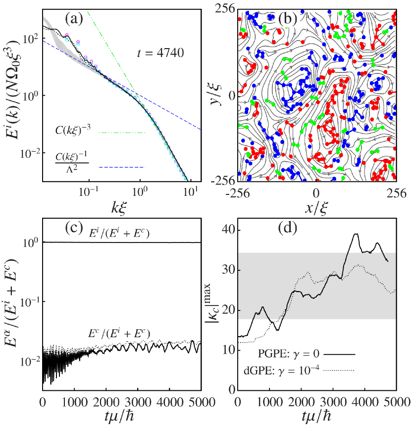
Figure 2: Dynamical PGPE evolution of a non-equilibrium neutral 384-vortex configuration (initial point-vortex energy per vortex $\varepsilon(t=0)=6$) towards an OKC state (see Fig. 2 of the main text). (a): IKE spectrum, compared to the statistical equilibrium distribution for $\varepsilon=6$ (grey shaded line, thickness indicates $\pm 1$ standard deviation). The solid black line and magenta circles show the time-averaged (over 500 natural time units $\mu/\hbar$) IKE spectrum obtained from the PGPE simulation using the point-vortex spectrum (Eq. 3 of main text) and the GPE, respectively. The dashed black line and cyan squares show the equivalent quantities from the dGPE simulation at the same time. (b): RCA decomposition (see main text) of the wavefunction in the PGPE simulation at time $t=4740\mu/\hbar$: the emerging OKC is clearly visible in the center of the field of view. (c): Comparison of the ratios of the total incompressible ($E^{i}$) and compressible ($E^{c}$) kinetic energies to the total kinetic energy $E^{i}+E^{c}$ in the PGPE (solid lines) and dGPE (dashed lines) simulations. In both cases, the initial compressible kinetic energy is extremely small and fluctuations due to numerical noise at high-$k$ are visible in the spectrum. At later times the compressible kinetic energy begins to grow, with faster growth occurring in the PGPE case. However, in both cases the compressible energy constitutes well below 5% of the total kinetic energy throughout the simulation. (d): Time-averaged absolute charge of the largest vortex cluster, $|\kappa_{c}|^{\rm max}$, for the PGPE (solid line) and dGPE (dashed line) simulations. Although the exact dynamics are different due to the chaotic nature of the vortex trajectories, both simulations show $|\kappa_{c}|^{\rm max}$ clearly moving toward the values expected in statistical equilibrium (shaded area).

The dGPE, with $\gamma$ treated as a more-or-less phenomenological parameter, has been widely-used as a description of finite-temperature Bose-Einstein condensates. Viewed phenomenologically, the dGPE’s key advantage is that it incorporates some of the dissipative physics lying beyond the zero-temperature GPE, while remaining computationally tractable even for large, complex systems Reeves et al. (2012). Within such a phenomenological treatment one can also attempt to heuristically include other effects by adjusting $\gamma$; for example in the case of the 2D dGPE considered here one might expect that the effects of coupling to compressible dynamics in the tightly-trapped $z$-direction could be phenomenologically captured by a higher effective damping rate $\gamma$. However, we emphasize that within the $c$-field approach $\gamma$ can be calculated a priori from experimental parameters, and typically has a value of order $10^{-4}$ Bradley and Anderson (2012). In this context, the dGPE simulations presented in our letter go beyond a phenomenological description. Indeed, recent works have shown that the dGPE can still give a qualitatively accurate picture of vortex dynamics in oblate-geometry persistent current formation experiments even at considerably high temperatures compared to $T_{c}$ Neely et al. (2013); Rooney et al. (2013).

The dynamical effects of the dissipation in the dGPE in the presence of quantum vortices are twofold: Firstly, the dissipation introduces a direct correction to the equations of motion for quantum vortices in a completely homogeneous background Törnkvist and Schröder (1997), introducing a velocity correction for each vortex proportional to $\gamma$ times the original (Hamiltonian) velocity. Secondly, the dissipation suppresses compressible energy at high wavenumbers $k$. Indeed, this effect is in some ways analogous to the effect of viscosity in the classical Navier-Stokes equations Bradley and Anderson (2012). The appearance of dissipative effects predominantly at wavenumbers $k>\xi^{-1}$ was confirmed numerically in simulations of beyond-mean-field dynamics using the Hartree-Fock-Bogoliubov description Kobayashi and Tsubota (2006). For the small value of $\gamma=10^{-4}$ used in our simulations the first of these effects is expected to be negligible over the integration time we consider ($t<10^{4}\mu/\hbar$). Thus, we expect damping to leave the vortex dynamics largely unaffected, while supressing sound energy at high $k$, and we expect our dGPE results for the vortex degrees of freedom to correspond closely to the Hamiltonian case.

IV.2 B. Relation to Hamiltonian (projected Gross–Pitaevskii) model

While the dissipative finite-temperature effects captured by the dGPE are likely to be present to some degree in any experimental realization of dynamical OKC formation, it is nonetheless interesting to consider what happens in the Hamiltonian case $\gamma=0$ numerically. Doing so provides confirmation that the vortex dynamics remain quantitatively similar in their statistical properties, and that dynamic OKC formation remains possible, in the limit of zero-temperature.

However, simulating the Hamiltonian evolution in a large, highly turbulent system is a significant numerical challenge. In the absence of damping, compressible energy transferred to high $k$ by the turbulent dynamics is not dissipated and must continue to be spatially and temporally resolved by the numerical method. This numerical challenge is similar to that of simulating condensate formation and inverse energy cascade in two-dimensional classical fluids McWilliams (1990); Chertkov et al. (2007); Xiao et al. (2009); Chan et al. (2012). As the central numerical difficulty lies in the aliasing of high-$k$ modes by the pseudospectral method Boyd (2000), the projected GPE (PGPE) Davis et al. (2001); Davis and Blakie (2006); Simula and Blakie (2006) is the appropriate framework for long-time simulations of Hamiltonian turbulence in a BEC. Within a $c$-field framework, the projector in the PGPE formally arises from quantum mechanical considerations; however, it is also directly connected to dealiasing procedures used in turbulent Navier–Stokes simulations (often in conjunction with a phenomenological hyperviscosity) Boyd (2000); Blakie (2008); Shukla et al. (2013).

Due to the large amount of computational time necessary for Hamiltonian simulations we have integrated the equations of motion up to the time $t\simeq 5000\mu/\hbar$, by which time the onset of OKC is clear in several measures. Figure 2 shows our results for the case $\varepsilon(0)=6$, obtained using a Fourier pseudospectral method for the undamped PGPE on a $4096^{2}$-point spatial grid with adaptive $4$th–$5$th order Runge-Kutta timestepping (relative error tolerance $10^{-6}$). See also the movies of dGPE and PGPE evolution accompanying this supplemental material. These results confirm the predictions of the dGPE [computed on a spatial grid of $2048^{2}$ points without a projector, with the same timestepping scheme], illustrating that dynamical OKC formation also occurs in the Hamiltonian case.