Energetic particle cross-field propagation early in a solar event

Abstract

Solar energetic particles (SEPs) have been observed to easily spread across heliographic longitudes, and the mechanisms responsible for this behaviour remain unclear. We use full-orbit simulations of a 10 MeV proton beam in a turbulent magnetic field to study to what extent the spread across the mean field can be described as diffusion early in a particle event. We compare the full-orbit code results to solutions of a Fokker-Planck equation including spatial and pitch angle diffusion, and of one including also propagation of the particles along random-walking magnetic field lines. We find that propagation of the particles along meandering field lines is the key process determining their cross-field spread at 1 AU at the beginning of the simulated event. The mean square displacement of the particles an hour after injection is an order of magnitude larger than that given by the diffusion model, indicating that models employing spatial cross-field diffusion cannot be used to describe early evolution of an SEP event. On the other hand, the diffusion of the particles from their initial field lines is negligible during the first 5 hours, which is consistent with the observations of SEP intensity dropouts. We conclude that modelling SEP events must take into account the particle propagation along meandering field lines for the first 20 hours of the event.

1. Introduction

Solar Energetic Particles (SEPs), accelerated during solar eruptive events, have been observed to have access to a wide range of heliographic longitudes, both for impulsive (Wiedenbeck et al. 2013) and gradual (Dresing et al. 2012) SEP events. In a number of studies, the spreading of SEPs across the field has been modelled using the Fokker-Planck (FP) equation for the particle distribution function (e.g., Jokipii 1966) with field-aligned propagation implemented as diffusion in velocity space, and cross-field propagation as spatial diffusion across the mean field (e.g., Zhang et al. 2009; Dröge et al. 2010; He et al. 2011). However, the cross-field diffusion coefficient $\kappa_{\perp}$ required to explain the SEP observations (e.g., Zhang et al. 2003; Dresing et al. 2012), is much larger than that derived from galactic cosmic ray observations (e.g. Burger et al. 2000) and full-orbit simulations (e.g. Giacalone & Jokipii 1999).

Matthaeus et al. (2003) used a model where the particles diffuse along field lines that random-walk across the mean magnetic field direction, to study the particle propagation across the mean magnetic field. They obtained $\kappa_{\perp}$ that is consistent with the galactic cosmic ray observations and full-orbit simulations. The diffusive behaviour of particles in this model is an asymptotic, long-time solution.

In this paper we study whether the need for a large $\kappa_{\perp}$ in the FP modelling of an SEP event is due to the fact that its description of cross-field diffusion may not be valid in the early phases of an SEP event. SEPs are observed at 1 AU soon after their injection, at only a few scattering mean free paths from their source (e.g. Palmer 1982). Thus the cross field spreading may not have settled to the asymptotic diffusive behaviour described by Matthaeus et al. (2003). Therefore, the question arises of whether a diffusion description for the initial SEP propagation is appropriate.

We study the early time cross-field transport of an SEP event by means of full-orbit simulations in a prescribed turbulence. We evaluate the early cross-field transport in this model and compare it quantitatively with that obtained from solution of a FP model.

Full-orbit models have been used to study charged particle propagation in turbulence superposed onto a constant background field to study the evolution and asymptotic values of the diffusion coefficients (e.g. Giacalone & Jokipii 1999; Qin 2002; Qin et al. 2002a, b; Laitinen et al. 2012, 2013), however not addressing the evolution of particle intensities at a fixed location. Giacalone et al. (2000) used a turbulence model in Parker spiral geometry to study the effect of the size of the SEP source region on the intensities observed at 1 AU, concluding that a small source region would result in intensity dropouts such as observed by Mazur et al. (e.g., 2000). In this study, however, we aim to quantify the efficiency of the particle cross-field transport in a statistical sense, and thus use a large source region.

To study the propagation early in an event, for simplicity we superimpose turbulence on a constant background magnetic field. We inject particles into the simulation as a beam, with pitch angle cosine $\mu=1$, to mimic the initial strong focusing of particles in the radial field close to the sun, as this mechanism is absent in constant magnetic field. We compare the result of this full-orbit simulation to a solution of a FP equation, and quantitatively show that the early evolution of an SEP event cannot be described using spatial cross-field diffusion in a FP equation. The early particle transport in the full-orbit simulations is consistent with particles propagating along meandering field lines. We demonstrate this by using a model that incorporates field line meandering into the FP method.

2. Models

2.1. Full-orbit simulations

The full-orbit simulations are based on the description of the turbulent magnetic field presented in Giacalone & Jokipii (1999), with

$$\mathbf{B}(x,y,z)=B_{0}\hat{\mathbf{z}}+\delta\mathbf{B}(x,y,z),$$ (1)

where $B_{0}$ is a constant background field, along the $z$-axis, and $\delta\mathbf{B}(x,y,z)$ a fluctuating field consisting of Fourier modes. We use $B_{0}=5$ nT, consistent with the field strength at 1 AU. For the fluctuations, we use the composite model, where turbulence is composed of slab and 2D components. We use a spectral index $\gamma=-1$ for the slab (1D) component, to prevent the so-called resonance gap issue which would complicate comparison with models using pitch angle diffusion, as discussed further in Section 2.2. The amplitude of the turbulence is set to give a parallel mean free path of 0.3 AU for a 10 MeV proton, a reasonable value for SEP protons (e.g., Palmer 1982). For the used spectral shape, the amplitude is somewhat lower than the interplanetary value, with parameter $B_{1}^{2}=0.1B_{0}^{2}$ (see Laitinen et al. 2012, for definition).

The full-orbit particle simulations follow the same approach as Laitinen et al. (2012). We start the particles in a large volume, to exclude the effects of coherence by close-by fieldlines discussed by, e.g., Giacalone et al. (2000) and Ruffolo et al. (2004). The quantities below are calculated relative to each particles’ initial position so that in coordinates $x$, $y$ and $z$ the initial position of each particle is at the origin. Thus, our study models statistically the spreading of particles from a large source region, excluding the effects of local field line coherence.

We calculate the perpendicular variance of the particles, $\sigma_{i}^{2}(z,t)=\left<(r_{\perp,i}(z,t)-\left<r_{\perp,i}(z,t)\right>)^{2}\right>$, where $r_{\perp,i}=x,y$ and $\left<\right>$ represents the ensemble average, as a function of time and location along the mean field. The local running perpendicular diffusion coefficient, $K_{\perp i}(z,t)$, is defined as

$$K_{\perp i}(z,t)=\frac{\sigma_{i}^{2}(z,t)}{2t},$$ (2)

and is obtained from particles within $z\pm\Delta z$, where $\Delta z=15r_{\odot}$, with $r_{\odot}$ the solar radius. These definitions of the perpendicular variance and local diffusion coefficient are not sensitive to the widening of the cross-field extent due to particles propagating along the mean field line: particles following their original field lines would produce a constant $\sigma_{i}^{2}(z,t)$, and any variation indicates decoupling of particles from the field lines (e.g. Hauff et al. 2010; Fraschetti & Jokipii 2011; Fraschetti & Giacalone 2012). Thus, $\sigma_{i}^{2}(z,t)$ is a powerful tool for determining the nature of the cross-field propagation of charged particles. It also better corresponds to what particle instruments observe: the intensities of particles at fixed locations, instead of the particle population’s full spatial extent.

We also calculate the standard asymptotic values of the diffusion coefficients as

$$\kappa_{i}=\lim_{t\rightarrow\infty}\frac{\left<\xi(t)^{2}\right>}{2t},$$ (3)

where $\xi(t)=x,y,z$, and the field line diffusion coefficient, due to the meandering of the turbulent field in Eq. (1), as

$$D_{\perp,\xi}=\lim_{z\rightarrow\infty}\frac{\left<\xi(z)^{2}\right>}{2z},$$ (4)

where $\xi(z)=x(z),y(z)$ are the coordinates of the field line at mean field direction distance $z$. These coefficients are used as input parameters in Sections 2.2 and 2.3.

2.2. Fokker-Planck test particle simulations

The second description of particle transport is based on a Fokker-Planck equation appropriate for our model definitions of static turbulence on constant background magnetic field, given by

$$\frac{\partial f}{\partial t}+\mu v\frac{\partial f}{\partial z}=\frac{\partial}{\partial\mu}D_{\mu\mu}\frac{\partial f}{\partial\mu}+\nabla\cdot\left(\hat{\kappa}_{\perp}\nabla f\right),$$ (5)

(e.g., Jokipii 1966; Schlickeiser 2002) where $f(x,y,z,v,\mu,t)$ is the particle distribution function, $v$ and $\mu$ the particle’s velocity and pitch angle cosine, $D_{\mu\mu}$ the pitch angle diffusion coefficient, and

$$\hat{\kappa}_{\perp}=\left(\begin{array}[]{ccc}\kappa_{\perp}&0&0\\ 0&\kappa_{\perp}&0\\ 0&0&0\end{array}\right)$$

the cross-field spatial diffusion tensor. This equation is solved via Monte Carlo test-particle simulations, using the approach described in e.g., Zhang et al. (2009) and Dröge et al. (2010). Below, this model is referred to with abbreviation FP.

The perpendicular diffusion of the particles, given by the last term in Eq. (5), is solved by means of stochastic differential equations (SDE) (Gardiner 1985), which gives the perpendicular Monte Carlo step for the particles as

$$dx = \sqrt{2\kappa_{\perp}dt}\,W_{x}$$ (6)

$$dy = \sqrt{2\kappa_{\perp}dt}\,W_{y}$$ (7)

where $W_{x}$ and $W_{y}$ are Gaussian random numbers with zero mean and unit variance, and $dt$ is the time step length.

The parallel propagation of the particles is given by

$$dz=\mu\,v\,dt$$ (8)

and the pitch angle is scattered isotropically using the method introduced by Torsti et al. (1996), with pitch angle diffusion coefficient

$$D_{\mu\mu}=\nu\left(1-\mu^{2}\right),$$ (9)

where the scattering frequency $\nu=v^{2}/(6\kappa_{\parallel})$ is independent of pitch angle for turbulence spectral index $\gamma=-1$ in quasilinear theory. This is chosen to avoid the problem of a resonance gap at small $\mu$ (see, e.g., Schlickeiser 2002), which would complicate comparison between the full-orbit simulations and the FP model.

We verified that the evolution of the pitch angle distribution obtained by using the pitch-angle diffusion method of Torsti et al. (1996) agrees well with that obtained from the full-orbit simulations, and thus we are confident that the propagation along the mean field lines is similar in the two methods. The two methods also agree well with the analytical solution to the isotropic pitch angle diffusion given by, e.g., Roelof (1969).

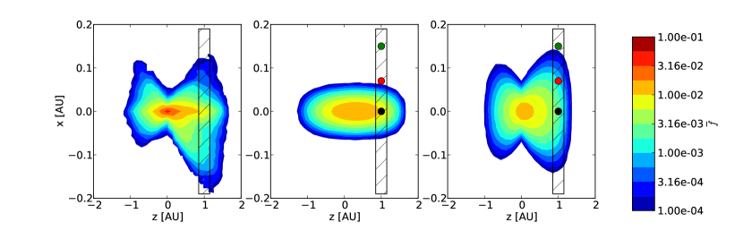
Figure 1.— Contour plot of the spatial SEP distribution for the full-orbit (left panel), FP (centre panel) and FP+FLRW (right panel) models at 115 minutes from the injection. The box at $z=1\pm 0.15$ AU depicts the range that is used for calculating the variance and local running diffusion coefficients in Figs. 2 and  3. The coloured circles correspond to the locations in Fig. 4.

2.3. Fokker-Planck test particle simulations with meandering field lines

In the third model, we add the effect of meandering field lines to the Fokker-Planck description of particle propagation introduced in Section 2.2. We model the field line wandering as diffusion, using the field line diffusion coefficient given by Eq. (4). We solve the path of the fieldline using the SDE approach, which gives

$$dx_{B} = \sqrt{2D_{\perp}dz_{B}}\,W_{x}$$ (10)

$$dy_{B} = \sqrt{2D_{\perp}dz_{B}}\,W_{y}.$$ (11)

We calculate the field line, $\left(x_{B}(z_{B}),y_{B}(z_{B}),z_{B})\right)$ separately for each particle. The particle will then propagate along this field line instead of the constant background field used in Section 2.2.

The meandering of the field line is taken into account by advancing the particle along the mean magnetic field direction by

$$dz=\mu\,v\,dt\,\cos\theta,$$

where $\theta$ is the angle between the mean field and the local meandering field. The diffusion step, given by Equations (6) and (7), is taken perpendicular to the meandering field line. The particle’s cross-field deviation from its initial location is composed of the diffusive propagation of the particle, $x(t)$ and $y(t)$, superimposed upon the wandering of the field line described by, $x_{B}(z(t))$ and $y_{B}(z(t))$. Below, this model will be referred to as FP+FLRW.

3. Results and Discussion

To analyse how energetic particles spread across the mean magnetic field in the three propagation models described above, we inject a population of 10 MeV protons with $\mu=1$ and follow them for 60 hours. The number of particles is $N=2\times 10^{5}$ in the full-orbit simulations, while the FP and FP+FLRW simulations use $N=2\times 10^{6}$ particles. The particle diffusion coefficients used in the FP and FP+FLRW models are the asymptotic values of the running diffusion coefficients of the full-orbit simulations, as given by Eq. (3). For this purpose, we simulate an isotropic proton population of N=2048 particles. For the turbulent field realisation presented in this study, we obtain a parallel diffusion coefficient $\kappa_{\parallel}=6.2\times 10^{21}\mathrm{cm}^{2}/\mathrm{s}$. The perpendicular diffusion coefficient is $\kappa_{\perp}=6.6\times 10^{18}\mathrm{cm}^{2}/\mathrm{s}$.

We also calculated the field line diffusion coefficient, $D_{\perp}=2.1\times 10^{10}\mathrm{cm}$, from the magnetic field lines used in the full-orbit simulations. This value is used to produce the field line random walk, with Eqs. (10)-(11).

We show the particle distribution with a contour plot in Fig. 1, for the full-orbit (left), FP (middle) and FP+FLRW simulations (right panel). The contours represent the particle distribution integrated along the $y$-direction, $\overline{f}(x,z,t)$, 115 minutes after injection, with the horizontal axis along the mean magnetic field. In the left panel particles on both the negative and positive $z$ region expand in the cross-field direction as they propagate farther from the origin along the $z$-axis. The particles with $z<0$ have been scattered back from the $z>0$ region, crossing the $z=0$ boundary close to the origin. This pattern of propagation can be expected for particles that follow field lines fanning out from the origin, while decoupling from their initial field line with a slow rate. The full-orbit particle distribution is distinctly different from the elliptical profile obtained with the FP model (middle panel), but qualitatively similar to the FP+FLRW model (right panel).

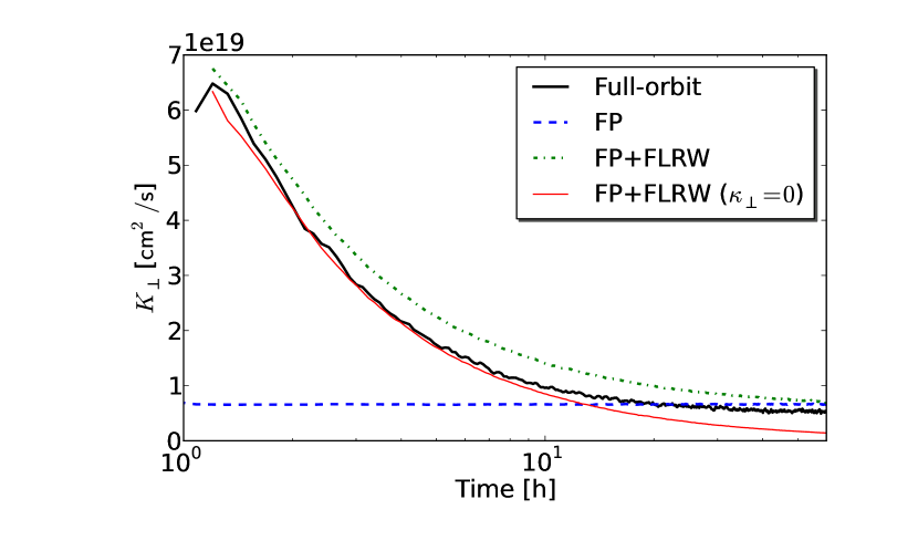
Figure 2.— The local running diffusion coefficient for the models, determined from particles at 1 AU from the injection location (the boxes in Fig. 1).

In Fig. 2 we show $K_{\perp}(z,t)$, as defined by Eq. (2), calculated using the particles in the range depicted by the boxes in Fig. 1. The temporal evolution of $K_{\perp}(z=1\mathrm{~{}AU},t)$ obtained with the FP model (blue dashed curve) differs considerably from the other models, staying at a constant value, as can be expected. In the full-orbit simulations (solid black curve), at the time of arrival of the first particles at 1 AU, about an hour after injection, $K_{\perp}$ is an order of magnitude larger than the FP value. The full-orbit $K_{\perp}$ reaches the level of the FP description only 10 hours after injection.

For the first 5 hours of the simulated event, the full-orbit diffusion coefficient follows closely the curve for a FP+FLRW model with $\kappa_{\perp}=0$ (red curve), which describes particles remaining on their original field lines. This can be seen more clearly in Fig. 3, where we show the evolution of the cross-field variance at 1 AU, $\sigma_{\perp}^{2}(z=\mbox{1 AU},t)$. The variance of the full-orbit simulated particles remains constant for the first 5 hours from injection, indicating that the FLRW effect dominates over particles decoupling from their field lines. As discussed by Giacalone & Jokipii (2012), the dominance of the field line meandering over the decoupling can explain the dropouts in SEP intensities observed in some impulsive events (e.g., Mazur et al. 2000; Chollet & Giacalone 2011). Only at later times does the decoupling of the particles from their initial field lines become non-negligible, and the full-orbit running diffusion coefficient approaches the FP+FLRW with non-zero perpendicular coefficient (the dash-dotted green curve in Figs. 2 and 3).

It should be noted that the non-monotonic behaviour and the small deviation from the red curve in the initial phase of the full-orbit simulations is caused by the local structures in the particular turbulence realisation; this behaviour varies between realisations.

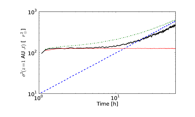
Figure 3.— The perpendicular variance of particles observed at 1 AU (the boxes in Fig. 1). For legend, see Fig. 2.

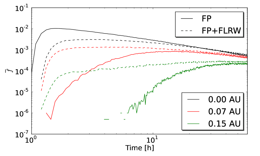
Figure 4.— Proton distribution function $\overline{f}(x,z,t)$ at the locations marked by black, red and green circles in Fig. 1, shown by black, red and green curves, respectively.

In Fig. 4, we show the evolution of $\overline{f}(x,z,t)$, at different cross-field locations $x$ at parallel distance $z=1$ AU from the injection location. The solid curves correspond to the FP model. We do not show the full-orbit simulations, as the local structure and asymmetries, evident from Fig. 1, are complicated and vary between turbulence realisations. Instead, we show the FP+FLRW model with non-zero $\kappa_{\perp}$ (dashed curves), which, of the FP models presented in this paper, best reproduces the evolution of the cross-field extent of the full-orbit simulated particles at 1 AU (Fig. 3).

At cross-field location $x=0$ AU (black curves), corresponding to a nominal connection to the injection site, the intensity evolution in the two models is similar. The FP+FLRW intensities are delayed by 15 minutes with respect to the FP model, due to the longer pathlength of the particle along the meandering field line. Full-orbit simulation onsets, not shown, variy somewhat with different realisations, due to varying field line lengths.

At a location not nominally connected to the injection site (red and green curves), the FP and FP+FLRW models show very different evolutions: while the FP+FLRW model shows rapid increase at wide cross-field range, the FP model displays significant delay in intensity onset, with a several-hour difference between the two models.

Our results thus suggest that the early evolution across the mean field is not diffusive, and using an incorrect model for the particle propagation may significantly distort the interpretation of the observed SEP intensities. The particles following the meandering field lines have access to large cross-field distances, compared to diffusively propagating particles, and arrive more promptly at the observing spacecraft if it is not magnetically well connected to the injection location. Using a spatial diffusion model to analyse such an event may result in either a large cross-field diffusion coefficient, or an interpretation of an extended acceleration region.

In this work, we introduced simplifications, such as the constant background magnetic field, to be able to compare different approaches with as few ambiguities as possible. Recent work by Giacalone & Jokipii (2012) found that in a Parker spiral geometry, spatial diffusion would be able to spread particles up to $180^{\circ}$ in longitude, and our results suggest that adding the meandering of field lines as in this study would aid the particles to fill the inner heliosphere with SEPs even further. The recently discussed effects of large-scale drifts for SEPs in Parker field may also increase the spread of SEPs in interplanetary space (Dalla et al. 2013; Marsh et al. 2013). On the other hand, the field line meandering may be limited by structures in the solar wind, as discussed by Laitinen et al. (2012). Also the adiabatic focusing and deceleration of the particles, occurring in the expanding corona, are important for SEP transport (e.g., Ruffolo 1995; Kocharov et al. 1998). Furthermore, the radial and spectral evolution of heliospheric turbulence (see, e.g., Cranmer & van Ballegooijen 2005, and references therein) will affect the spreading of particles in interplanetary space.

We also note that the method of calculating the cross-field variance at a fixed distance along the mean field from the initial position, $\sigma^{2}(z,t)$, may be useful for studying the rate at which particles decouple from the field lines. Decoupling can be clearly seen at $z=0$ in the left panel of Fig. 1: the cross-field spreading around $x=0,z=0$ is caused by the decoupling, and the rate can be measured using the approach introduced in this work. As can be seen in Fig. 2, a constant spatial diffusion coefficient, as used in the FP+FLRW model, cannot describe this spreading. It is likely that the spreading is connected to the evolution of the field line separation (see Ruffolo et al. 2004) after the particle has moved to a different field line.

4. Conclusions

In this work, we have studied particle propagation across the mean field as a function of time, after an impulsive, beam-like injection into a turbulent magnetic field. We compared the spatial evolution of energetic particles using three simulation methods: full-orbit particle simulations using synthetic meandering field lines, spatial and pitch angle diffusion along constant background field (FP), and diffusive propagation along stochastically spreading field lines (FP+FLRW). Our main findings are as follows:

• The propagation of particles across the mean magnetic field in the early phase of an event is mainly due to the particles following meandering magnetic fields, resulting in cross-field mean square width an order of magnitude larger than that predicted by a diffusion model. This behaviour of the particle propagation cannot be described as a cross-field diffusion across mean magnetic field, but requires a description for the meandering field lines.

• The large cross-field spread of the particles at the time of arrival of the first particles (Fig. 3) may explain the observations of SEPs at wide longitudinal separation, as reported by, e.g., Dresing et al. (2012) and Wiedenbeck et al. (2013).

• The timing of the access to field lines at large cross-field distances is rapid in a description including FLRW (red and green dashed curves in Fig. 4), and takes place much faster than in a model including diffusion only.

Early in an event the particles remain well on their initial field lines, and thus do not propagate across the meandering field lines (see Figs. 2 and 4). A vanishingly small cross-field diffusion coefficient during impulsive “dropout” events has been previously suggested based on FP simulations (Dröge et al. 2010) and observations (Chollet & Giacalone 2011). We find, based on our simulations, that a small diffusion coefficient early in an SEP event is not contradicted by a larger diffusion coefficient later in the event.

We conclude that in modelling of an SEP event, the description of cross-field propagation as spatial diffusion only is not sufficient, and a description of field line meandering should be used. Adding FLRW to the standard FP description, as presented in this paper, is a reasonable method to model the particle propagation as seen in the full orbit simulations. However, the spatial cross-field diffusion from the meandering field lines is very slow during the first hours of the event, approaching the asymptotic diffusion coefficient only at later times. Thus, a model with time-dependent diffusion coefficient is needed to accurately describe the particle decoupling from their initial field lines.

References

- Burger et al. (2000) Burger, R. A., Potgieter, M. S., & Heber, B. 2000, J. Geophys. Res., 105, 27447
- Chollet & Giacalone (2011) Chollet, E. E., & Giacalone, J. 2011, ApJ, 728, 64
- Cranmer & van Ballegooijen (2005) Cranmer, S. R., & van Ballegooijen, A. A. 2005, ApJS, 156, 265
- Dalla et al. (2013) Dalla, S., Marsh, M., Kelly, J., & Laitinen, T. 2013, JGR (Space Physics), submitted
- Dresing et al. (2012) Dresing, N., Gómez-Herrero, R., Klassen, A., Heber, B., Kartavykh, Y., & Dröge, W. 2012, Sol. Phys., 281, 281
- Dröge et al. (2010) Dröge, W., Kartavykh, Y. Y., Klecker, B., & Kovaltsov, G. A. 2010, ApJ, 709, 912
- Fraschetti & Giacalone (2012) Fraschetti, F., & Giacalone, J. 2012, ApJ, 755, 114
- Fraschetti & Jokipii (2011) Fraschetti, F., & Jokipii, J. R. 2011, ApJ, 734, 83
- Gardiner (1985) Gardiner, C. W. 1985, Handbook of Stochastic Methods (Berlin: Springer)
- Giacalone & Jokipii (1999) Giacalone, J., & Jokipii, J. R. 1999, ApJ, 520, 204
- Giacalone & Jokipii (2012) —. 2012, ApJ, 751, L33
- Giacalone et al. (2000) Giacalone, J., Jokipii, J. R., & Mazur, J. E. 2000, ApJ, 532, L75
- Hauff et al. (2010) Hauff, T., Jenko, F., Shalchi, A., & Schlickeiser, R. 2010, ApJ, 711, 997
- He et al. (2011) He, H.-Q., Qin, G., & Zhang, M. 2011, ApJ, 734, 74
- Jokipii (1966) Jokipii, J. R. 1966, ApJ, 146, 480
- Kocharov et al. (1998) Kocharov, L., Vainio, R., Kovaltsov, G. A., & Torsti, J. 1998, Sol. Phys., 182, 195
- Laitinen et al. (2012) Laitinen, T., Dalla, S., & Kelly, J. 2012, ApJ, 749, 103
- Laitinen et al. (2013) Laitinen, T., Dalla, S., Kelly, J., & Marsh, M. 2013, ApJ, 764, 168
- Marsh et al. (2013) Marsh, M., Dalla, S., Kelly, J., & Laitinen, T. 2013, ApJ, submitted
- Matthaeus et al. (2003) Matthaeus, W. H., Qin, G., Bieber, J. W., & Zank, G. P. 2003, ApJ, 590, L53
- Mazur et al. (2000) Mazur, J. E., Mason, G. M., Dwyer, J. R., Giacalone, J., Jokipii, J. R., & Stone, E. C. 2000, ApJ, 532, L79
- Palmer (1982) Palmer, I. D. 1982, Reviews of Geophysics and Space Physics, 20, 335
- Qin (2002) Qin, G. 2002, PhD thesis, University of Delaware
- Qin et al. (2002a) Qin, G., Matthaeus, W. H., & Bieber, J. W. 2002a, ApJ, 578, L117
- Qin et al. (2002b) —. 2002b, Geophys. Res. Lett., 29, 1048
- Roelof (1969) Roelof, E. C. 1969, in Lectures in High-Energy Astrophysics, ed. H. Ögelman & J. R. Wayland, 111
- Ruffolo (1995) Ruffolo, D. 1995, ApJ, 442, 861
- Ruffolo et al. (2004) Ruffolo, D., Matthaeus, W. H., & Chuychai, P. 2004, ApJ, 614, 420
- Schlickeiser (2002) Schlickeiser, R. 2002, Cosmic Ray Astrophysics (Springer)
- Torsti et al. (1996) Torsti, J., Kocharov, L. G., Vainio, R., Anttila, A., & Kovaltsov, G. A. 1996, Sol. Phys., 166, 135
- Wiedenbeck et al. (2013) Wiedenbeck, M. E., Mason, G. M., Cohen, C. M. S., Nitta, N. V., Gómez-Herrero, R., & Haggerty, D. K. 2013, ApJ, 762, 54
- Zhang et al. (2003) Zhang, M., Jokipii, J. R., & McKibben, R. B. 2003, ApJ, 595, 493
- Zhang et al. (2009) Zhang, M., Qin, G., & Rassoul, H. 2009, ApJ, 692, 109